Temporal evolution of the momentum balance terms and frictional
adjustment observed over the inner shelf during a storm
M. Grifoll1,2, A. L. Aretxabaleta3, J. L. Pelegrí4, and M. Espino1,2 1Technical University of Catalonia, Barcelona, Spain
2International Centre of Coastal Resources Research, Barcelona, Spain 3US Geological Survey, Woods Hole, MA, USA
4Departament d’Oceanografia Física i Tecnològica, Institut de Ciències del Mar, CSIC, Barcelona, Spain
Correspondence to:M. Grifoll ([email protected])
Received: 27 April 2015 – Published in Ocean Sci. Discuss.: 27 May 2015
Revised: 16 December 2015 – Accepted: 21 December 2015 – Published: 18 January 2016
Abstract. We investigate the rapidly changing equilibrium between the momentum sources and sinks during the pas-sage of a single two-peak storm over the Catalan inner shelf (NW Mediterranean Sea). Velocity measurements at 24 m water depth are taken as representative of the inner shelf, and the cross-shelf variability is explored with measurements at 50 m water depth. During both wind pulses, the flow accel-erated at 24 m until shortly after the wind maxima, when the bottom stress was able to compensate for the wind stress. Concurrently, the sea level also responded, with the pressure-gradient force opposing the wind stress. Before, during and after the second wind pulse, there were velocity fluctuations with both super- and sub-inertial periods likely associated with transient coastal waves. Throughout the storm, the Cori-olis force and wave radiation stresses were relatively unim-portant in the along-shelf momentum balance. The frictional adjustment timescale was around 10 h, consistent with thee
-folding time obtained from bottom drag parameterizations. The momentum evolution at 50 m showed a larger influence of the Coriolis force at the expense of a decreased frictional relevance, typical in the transition from the inner to the mid-shelf.
1 Introduction
The inner shelf, encompassing depths ranging from a few to tens of meters, is dynamically defined as the region that lies between the surf zone (where waves break and the mo-mentum balance is dominated by wave-induced terms) and
the mid-shelf (where the along-shelf circulation is usually in geostrophic balance) (Lentz and Fewings, 2012). The circu-lation over the inner shelf is often investigated through the analysis of the momentum balance in different regions, al-though most studies have usually focused on those condi-tions averaged over periods longer than 1 week (Lee et al., 1984; Lentz and Winant, 1986; Lentz et al., 1999, Maza et al., 2006; Fewings and Lentz, 2010; Grifoll et al., 2012, 2013). In contrast, the analysis of the momentum terms at daily and shorter timescales under rapidly changing forcing conditions remains less explored.
sea-level slope opposing the wind stress in order to estab-lish a frictional equilibrium that differed from the average conditions. A seasonal study of the Catalan shelf (Grifoll et al., 2013) suggested that the occurrence of one single intense event can dominate the monthly averaged momentum bal-ance, with water piling against the coast as a response to the enhanced wind stress; to balance the surface forcing, the bot-tom stress term was also increased.
In this paper, we investigate the temporal evolution of the momentum balance terms over relatively short timescales (of order 1 day) during the passage of a storm. The anal-ysis is based on a set of observations from the Catalan in-ner shelf (offshore the city of Barcelona, NW Mediterranean Sea; Fig. 1). The prevalent momentum terms at two different depths (24 and 50 m) are examined. We take advantage of our setting in a micro-tidal environment to investigate a temporal scale (from hours to a few days) usually not considered in the literature, where the time series are often low-pass filtered to remove the short-term fluctuations (e.g., tidal flow). The goal is to quantify the different momentum terms during the storm and to examine the response timescales of the inner-shelf en-vironment to the principal forcing mechanisms.
2 Site location, data and methods
The Catalan shelf is micro-tidal, with tidal amplitudes of the order of 0.1 m. The wind and heat flux regimes exhibit a seasonal cycle associated with the Mediterranean climate and the periodicity of meteorological events in the region. Wind intensity usually has a minimum during summer and is more energetic during fall, winter and spring. During these last seasons, regional storms are predominantly associated with north and northeast winds alternating with northwest-erly wind pulses (land winds). Grifoll et al. (2013) analyzed the resulting seasonal circulation pattern over the inner shelf through a combination of numerical and observational tech-niques. The flow is prevalent in the along-shelf direction year-round, which is consistent with the coastal constraint and the shallowness of the area. The monthly averaged along-shelf momentum balance was between wind stress and pres-sure gradient, with bottom stress being a second-order term. In the present study, we focus on a subset of the data ana-lyzed by Grifoll et al. (2012) that includes an energetic event lasting a few days during March 2011. The bulk of the mea-surements correspond to a field experiment conducted over the Catalan inner shelf in the framework of the FIELD_AC project (Grifoll et al., 2012). The data set consisted of ve-locity time series from three Acoustic Doppler Current Pro-filer (ADCP) deployments, each with a pressure sensor (A1 [AWAC], A2 [AWAC] and A3 [RDI]; Fig. 1). The ADCP bin size was 1 m for A1 and A2, and 2 m for A3 station; the ve-locity accuracy was ±0.5 cm s−1. The along-shelf distance
between A1 and A2 was 4 km. A1 and A2 were deployed less than 1 km from the coast (24 m bottom depth) while A3
was 3 km away from the coast (50 m bottom depth). Wind data were collected using a mast located at a Coastal Station Observatory (CSO; www.pontdelpetroli.org; see Fig. 1). In addition, 43 conductivity-temperature-depth (CTD) profiles were collected between 17 March and 10 April 2011 in the area surrounding the ADCPs (Grifoll et al., 2012, described the temperature and salinity conditions). Additionally, syn-optic information for the storm (winds and sea-level pres-sure) was obtained from the ERA-Interim global reanalysis product by the European Centre for Medium Range Weather Forecasting (ECMWF).
Wave data were recorded through a directional wave buoy [Datawell DWR-G7] moored at A3. A numerical wave model SWAN (Booij et al., 1999) was implemented and calibrated for a region that covers our study area, providing the wave variables with 50 m resolution to estimate the wave-induced momentum terms. The numerical domain is shown in Fig. 1 and the implementation details were presented in Grifoll et al. (2014).
The time series used for estimating the momentum terms have been low-pass filtered with a 1/12 h−1cutoff frequency to avoid short time fluctuations. This choice of filter win-dow is a compromise that allows for capturing momentum changes in timescales as short as 6 h and still removing short fluctuations, from minutes to a few hours. It is also consistent with observations of low energy at frequencies much higher than inertial (Grifoll et al., 2012).
3 Results
3.1 Event description
The currents during the entire March–April 2011 field cam-paign were analyzed in a previous study (Grifoll et al., 2012), highlighting the prevalence of the along-shelf direction and the high correlation between the velocities measured at A1, A2 and A3. For this reason, we focus on the A2 observations, considered to be representative of the dynamics in the inner shelf, and use A1 and A3 to support the momentum-term es-timates. The investigation of the cross-shelf variability in the along-shelf momentum equation also uses A3.
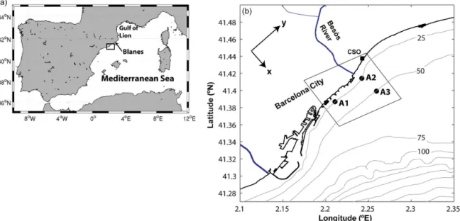
low-Figure 1.Map of the western Mediterranean Sea with the study area(a).(b)Shows the bathymetry of a portion of the Catalan shelf (isobaths every 25 m) with the locations of the ADCP sensors (A1, A2 and A3). A directional wave buoy was placed at A3. The square marker shows the Coastal Station Observatory (CSO) where the wind data were recorded.(b)Includes the numerical model domain used to propagate the wave conditions into A2 (black rectangle); the reference system adopted for the momentum balance is also shown.
pressure center over the study area. The storm finished on 15 March when the wind intensity decreased to zero.
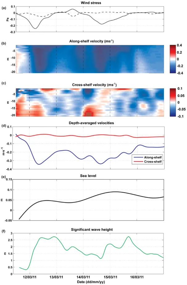
The along-shelf velocity (Fig. 3b) was characterized by a prevalent southwestward flow in the entire water column, with near-surface velocities typically 4 times larger than the near-bottom flow. The cross-shelf flow (Fig. 3c) was less in-tense than the along-shelf flow and exhibited a complex ver-tical structure. As a result, the depth-averaged along-shelf velocities were much larger than the depth-averaged cross-shelf velocities during the two wind peaks (Fig. 3d), reflect-ing a strong flow polarization associated with the coastal con-straint.
During the first day of the storm (12 March), the depth-averaged along-shelf current (Fig. 3d) was toward the south-west with a maximum at 07:00 UTC (2 hours after the wind stress peak). During the calm day (13 March 00:00– 22:00 UTC), the wind changed direction slightly toward the northeast (peaking at 15:00 UTC), but the along-shelf cur-rents maintained a similar magnitude and structure than the day before. During the second wind peak the situation re-peated itself, but with the along-shelf flow displaying some oscillations. The wind measurements are in good agreement with the values expected from the synoptic charts in Fig. 2.
The cross-shelf currents also displayed a similar time evo-lution during both wind peaks: the cross-shelf flow inten-sified with the wind, onshore at the surface and offshore near the bottom; as the wind stress decreased, the flow re-versed, turning offshore at the surface and onshore near the bottom (Fig. 3d). During the calm day, the cross-shelf flow was weakly onshore. Following the second wind peak (14 March 16:00 UTC), the surface wind stress decreased
gradually from 0.2 Pa to zero (15 March 23:00 UTC). The along-shelf flow remained to the southwest throughout the water column, and the cross-shelf flow was offshore in the sub-surface layers balanced by onshore currents near bottom. The detided sea level (Fig. 3e) increased during both wind peaks and slowly decreased after the last wind peak. After the storm, the sea level increased as a result of water being piled up against the coast due to the northeasterly wind. The wave conditions measured at A3 were characterized by two significant wave height peaks (Fig. 3f) from the E–SE di-rection with 8 s period. The peaks of significant wave height followed the peaks of (along-shelf) wind stress, with a delay longer than for the along-shelf currents because of the influ-ence of swell.
3.2 Momentum balance in the inner shelf
Assuming hydrostatic balance, ignoring the sea-level varia-tions as compared with the total water depth, and neglect-ing the baroclinic terms (estimated as small in Grifoll et al., 2012, 2013), the depth-averaged along-shelf momentum bal-ance equation can be written as
∂v¯ ∂t |{z}
ACCE.
+∂∂yv¯v¯+∂∂xu¯v¯ | {z }
ADVEC.
+vH¯v¯∂H∂y +u¯Hv¯∂H∂x
| {z }
CROS.SLP.
+ fu¯ |{z}
COR.
= −g∂n ∂y | {z }
PRS.GRD.
+ ρHτys |{z}
W.STR.
− ρHτyb |{z}
B.STR.
−ρH1 ∂S
yy ∂y +
∂Sxy ∂x
| {z }
RAD.STR.
, (1)
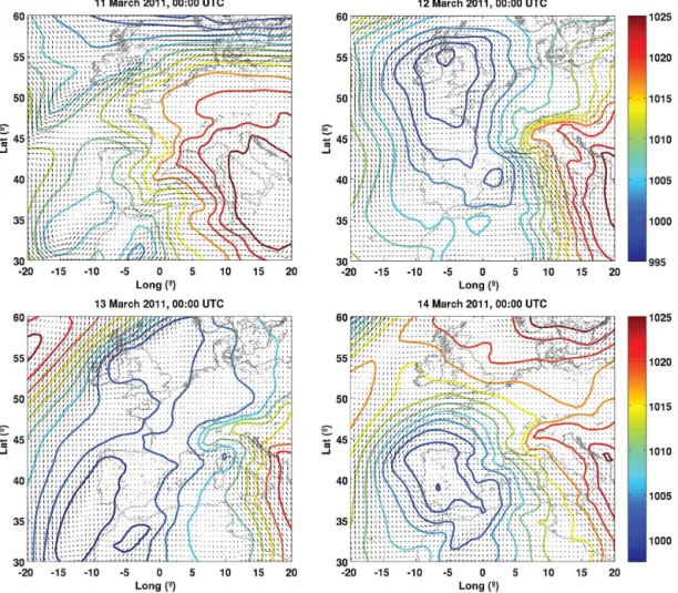
Figure 2.Regional charts of the mean sea-level pressure (HPa) and winds for the sequence 11–14 March 2011. Data source: ERA-Interim
global reanalysis from ECMWF.
the Coriolis parameter (f =9.6×10⁻⁵s−1),ρ is the water density (1025 kg m−3),ηis the sea-level perturbation asso-ciated with the barotropic component of the flow,τys is the along-shelf wind stress,τybis the along-shelf bottom stress and Syy, Sxy represent the wave-induced mass fluxes esti-mated via radiation stresses (Longuet-Higgins and Stewart, 1964).
The along-shelf acceleration term at A2 (ACCE. in Eq. 1) is estimated from the observations using finite-centered dif-ferences with the velocity recorded at A2 (Fig. 4a). A neg-ative peak is observed in the acceleration time series dur-ing the first wind peak. Durdur-ing 13 March, about 1 day after the first wind peak and shortly after the wind weakened (and even reversed), the acceleration term displayed an oscillatory pattern with a repeat interval of about 1 day or less.
The non-linear or advective terms are estimated by finite differentiation between the adjacent ADCP measurements (Kirincich and Barth, 2009; Fig. 4b). The velocity advection terms (ADVEC. in Eq. 1) were small during the first peak of the storm but later oscillated in a manner similar to the
acceleration term. There are two additional momentum ad-vection terms related to changes in the depth of the water column: u¯v¯
H
∂H
∂x + ¯ vv¯ H
∂H
∂y. The first term, the cross-shelf slope term (CROS.SLP.), has to be retained in our analysis, while the second term is zero, as the water depth is constant in the along-shelf direction.
The Coriolis term (COR in Eq. 1), computed from the depth-averaged cross-shelf velocities at A2, is small in com-parison with the acceleration term during the storm (Fig. 4c). Although the surface and sub-surface cross-shelf flows were relatively important through the water column (Fig. 3c), the depth-averaged cross-shelf flow was much smaller than the along-shelf velocities (Fig. 3d). The size of this term was 4 times smaller than the acceleration term.
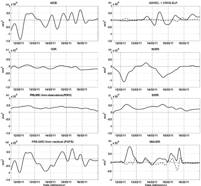
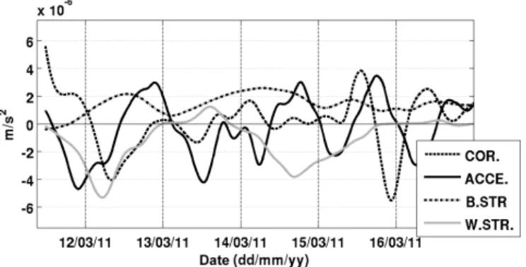
Figure 4.Estimates for the along-shelf momentum terms at 25 m. Left-hand-side terms of Eq. (1):(a)acceleration terms (ACCE.δv/δt ), (b)advective (solid line, ADVEC.,δv2/δy+δ(vu)/δx) and cross-slope (dashed line, CROS.SLP., (uv/H ) δH /δx) terms estimated from the currents at the neighboring ADCP locations and(c)Coriolis term (COR.,f u). Right-hand-side terms of Eq. (1):(d)wind stress term
(W.STR.,τys/ρH ),(e)pressure-gradient force from observations (PGFO term,gδη/δy),(f) bottom stress term (B.STR.,τyb/ρH ),(g)
pressure-gradient force from residual (PGFR) and(h)radiation stress term (RAD.ST., (1/ρH )δSxy/δx solid line, and (1/ρH)δSyy/δy
dashed line). Notice the change in the vertical scale in panel(h). The data used for estimating the momentum terms have been low-pass
filtered, with a cutoff period of 12 h. The date indicates 00:00 UTC.
few hours before the maximum winds (12 March 05:00 and 12 March 7:00 UTC). After the first wind peak, the accelera-tion decreased rapidly and changed sign, becoming small but positive during the remaining of the wind pulse. Something similar happened during the second wind peak, but this time characterized by several fluctuations, with acceleration peaks occurring about every 24 h or less (Fig. 4a).
The bottom stress (B.STR. in Eq. 1) is estimated using a linear drag law (Lentz and Winant, 1986):
τys=ρ r vb, (2)
where r is the linear drag coefficient, ρ is density andvb is the near-bottom velocity (measured at about 1 m from
formula-immediately after the peak wind stress (Fig. 4e).
The wave-induced mass fluxes (RAD.STR. in Eq. 1) are estimated as follows:
Sxy=E cg
csinφcosφ, (3)
Syy=E
cg
c
1+sin2φ−1 2
, (4)
where the wave energy is computed as E=ρ0gHsig2 /16, withHsig as the significant wave height,φ the wave direc-tion of propagadirec-tion, and cg and c, respectively the (linear theory) group and phase velocity at the peak wave frequency. Model radiation stress gradients are then estimated from two adjacent numerical cells in the proximity of A2 that consid-ered the propagation of wave conditions measured at A3. The peak values in significant wave height (about 2.5 m), and hence in the radiation stresses, occurred slightly after the maximum winds because of swell effects (Fig. 4h). The ra-diation stress terms were 1 order of magnitude smaller than the dominant frictional and acceleration terms.
No direct estimate of the along-shelf pressure-gradient force (PRS.GRD. in Eq. 1) can be obtained from the data. The ADCP recorded the pressure in the water column but the distances between ADCPs are not appropriate to capture the along-shelf sea-level variability, as the signal-to-noise ra-tio is not adequate. Hickey (1984) pointed out that, for spa-tial scales of the same order of magnitude as the external Rossby radius (about 100 km in the Catalan Sea), the ex-pected sea-level gradient would be only a few centimeters. In our case, the sea-level variations recorded by the pair of pressure sensors in A1 and A2 (separated by only a few kilo-meters) were of the same order as the accuracy of the de-vices (order millimeters). As an alternative approximation, an observed pressure-gradient force (PGFO) may be com-puted using data from a sea-level gauge located in the harbor of Blanes (approximately 64 km to the north; Fig. 1) and the ADCP pressure sensor at A2. This along-shelf pressure gra-dient remained positive during the entire storm, meaning a downwind accumulation of water, and was reinforced during the two wind peaks (Fig. 4e).
Additionally, we may calculate this along-shelf pressure-gradient force as the residual from the momentum balance equation (PGFR) as follows:
PGFR=∂v¯ ∂t +
∂v¯v¯
∂y + ∂u¯v¯
∂x + ¯ uv¯
H ∂H
∂x +fu¯− τys ρH
+ τyb ρH + 1 ρH ∂Syy ∂y + ∂Sxy ∂x . (5)
Maza et al. (2006) used a similar approach to compute the pressure-gradient force when the sea-level gradient was not
is consistent with the evolution of the momentum balance. The resulting coefficient is 8.5×10⁻⁴m s−1, comparable to
values computed from observations at similar depths (Winant and Beardsley, 1979).
Both the observed and residual pressure-gradient time se-ries (PGFO and PGFR) reproduce the force direction of the sea-level slope during the wind stress peaks (Fig. 4d). The PGFR includes a contribution by a direct response to the lo-cal wind forcing (for instance during 13 March), which is not immediately obvious in PGFO. During the wind peaks, the positive pressure-gradient force partially counterbalanced the wind stress in a manner consistent with other observational studies (Lee et al., 1984; Lentz, 1994; Fewings and Lentz, 2010). Despite its potentially large uncertainty, we use PGFR in the analysis of the momentum balance evolution because it is consistent with the estimates for the other momentum terms.
3.3 Momentum balance near the mid-shelf
The cross-shelf variability of the along-shelf momentum is estimated by comparing the inner-shelf results with the mo-mentum terms at 50 m water depth. The acceleration and bot-tom stress follow a pattern similar to the one observed at 24 m (Fig. 5). During the first wind peak, the acceleration responded to the wind stress, with its maximum occurring before the maximum winds. The maximum bottom stress, as at 24 m, occurred a few hours after the maximum winds. Dur-ing the second peak, the situation was less clear than at 24 m, with substantial oscillations in the acceleration and bottom stress. The bottom stress reached a minimum toward the end of the negative wind stress pulse.
From the velocities observed at A3, we estimate the sur-face and bottom frictional forces, the acceleration and the Coriolis force (Fig. 5). The surface stress term is estimated with the local wind measured at the CSO, scaled with the cor-responding water depth. The non-linear terms cannot be es-timated due to the lack of additional measurements at 50 m, necessary to assess the along-shelf gradient. Thus, as the ad-vective and wave-radiation terms are not available, we es-timate the pressure gradient as a residual that results from combining acceleration, Coriolis and wind and bottom fric-tion (PGFRACCE+COR+FRIC):
PGFRACCE+COR+FRIC=∂v¯
∂t +fu¯− τys ρH +
τyb
ρH. (6)
Figure 5.Estimates for the along-shelf momentum terms at 50 m.
Left-hand-side terms of Equation 1: acceleration terms (ACCE.
δv/δt) and Coriolis (COR. fu). Right-hand-side terms of
Equa-tion 1: wind stress term (W.STR.τys/ρH) and bottom stress term
(B.STR. –τyb/ρH). The data used for estimating the momentum
terms have been low-pass filtered with a cutoff period of 12 h. The date indicates 00:00 UTC.
4 Discussion
4.1 Momentum evolution in the inner shelf
From the estimated along-shelf momentum terms, we con-clude that the primary balance at 24 m (Fig. 4) took place be-tween acceleration, wind stress, bottom friction, momentum advection and pressure force gradient. The Coriolis force and the radiation stress played secondary roles in the momentum balance. In particular, the radiation stresses were 1 order of magnitude smaller than the dominant acceleration, pressure gradient and frictional terms, consistent with other studies that ignored wave forcing outside the surf zone (Lentz et al., 1999; Fewings and Lentz, 2010). In a region 150 km north of our study area, in water depths of 28 m off the Tet River, Michaud et al. (2012) confirmed numerically that the wave effects on the inner-shelf circulation are relatively small even during a storm event.
While our estimates present some uncertainty as a result of instrumental inaccuracies and the intrinsic assumptions in the estimation of the terms, we expect them to be reasonable approximations to the relative size of the dominant terms in the time-varying along-shelf momentum balance. In this sec-tion, we combine the wind and velocity observations with the along-shelf momentum estimates to further analyze the inner-shelf response to the changing winds.
During the first peak (12 March), as the wind stress in-creased, the acceleration term initially became more nega-tive and the bottom stress more posinega-tive, as expected from the direction of the flow (Fig. 4a). The peak in the acceler-ation term occurred 4 h before the wind maximum, as a re-sult of the enhanced frictional dissipation and a rapid change in the residual pressure-gradient force (PGFR), from nega-tive to posinega-tive values (Fig. 4a, f and g). The change in the sign of PGFR, indicative of downwind water accumulation,
was abrupt, being responsible for switching the acceleration from negative to positive at about 10:00 UTC, hence set-ting the size and timing of the maximum along-shelf current (Fig. 3d).
During the calm period (13 March), the PGFR once again reversed, likely caused by a relaxation after the first wind peak. The acceleration remained close to zero until 13 March 10:00 UTC and then turned negative, despite the appearance of weak northeast winds. The negative acceleration started at the time when onshore winds were observed (Fig. 3a). The intensification of the southwestward PGFR was locally re-flected by a leveling of the sea surface throughout 13 March (Fig. 3e). The sequence of events is consistent with the in-tensification of a southwestward flow probably in cross-shelf geostrophic balance. During 14 March, when both along-and cross-shelf winds were weak, some nearshore water was progressively released, first through a two-layer baroclinic cross-shelf flow and then by offshore flow in the entire water column (Fig. 3c).
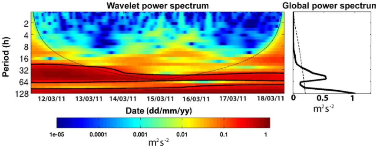
The along-shelf momentum balance during the second wind peak shared some characteristics with the balance dur-ing the first wind peak but also displayed important differ-ences. The acceleration term and the PGFR were enhanced following the increase in wind stress, with the along-shelf velocity reaching a maximum at the time of the second wind peak. However, the second wind event also had substantial fluctuations in the acceleration, advective, bottom friction, Coriolis and PGFR terms (Fig. 4). The fluctuations appear as a moderate increase in energy at the 12–16 h band in the wavelet analysis for the depth-averaged currents at station A2 (Fig. 6). These oscillations are consistent with fluctuations in the lowest part of the water column in the cross-shelf veloc-ities (Fig. 3c), and could be explained as a transient coastal current response to the sudden enhanced wind stress in the form of inertio-gravity waves (Kundu et al., 1983; Tintoré et al., 1995). These waves are associated with near-inertial motions resulting from the flow adjustment at the coast. An-other plausible explanation of these oscillations is the gen-eration of internal waves dispersed from the surface (wind-mixed layer) to larger depths in the lee of the storm (Gill, 1982; Kundu and Thompson, 1985) or fast coastal Kelvin waves (Csanady, 1982; Gill, 1982). Their proper characteri-zation would require additional observations in the cross- and along-shelf directions jointly with more detailed information of the stratification in the water column before and after the storm.
Figure 6.(Left) wavelet analysis and (right) spectral analysis for the depth-averaged currents at station A2. The solid thin line in the wavelet
power spectrum shows the energy values that exceed the significance level; similarly, the dashed line in the global power spectrum shows the significance level. The date indicates 00:00 UTC.
linear and frictionless coastal band. The theoretical lowest-mode topographic waves have a period of about 32 h, which is similar to the dominant period as deduced from the spectral and wavelet analyses (Fig. 6). Observed sea-level oscillations (Fig. 3e), as large as 0.05 m on timescales of about 1–2 days, gave rise to velocities of about 0.3 m s−1(Fig. 3c). Jordi et al. (2005) described the existence of topographic waves in the NW Mediterranean Sea, which propagated southwest. Due to our limited observations, additional measurements and nu-merical modeling efforts (e.g., Brink and Chapman, 1985) are necessary to properly characterize the relevance of topo-graphic waves during storms.
The differences between the observed and residual pressure-gradient forces, PGFO and PGFR, are striking (Fig. 3). The PGFR is necessary to balance the flow yet it differs substantially from the pressure gradient as calcu-lated from the A2 and Blanes sea-level gauges (64 km apart). Hence, we may interpret the PGFR as composed of two con-tributions: (1) a rapid coastal response to the along- and cross-shelf wind forcing, and (2) a relatively slow sea-level adjustment to the propagating storm. Our interpretation is that the PGFO corresponds to the second, relatively smooth, contribution, which would drive the flow in the absence of waves (as it occurs during the first wind event).
Our analysis highlights the importance of the initial con-ditions (whether the system starts from rest or not) and the complexity of the momentum fluctuations during the devel-opment of the storm. A comparison of the temporal evolu-tion of the momentum terms during both wind peaks shows that the role of the acceleration and advective terms is quite different. During the first peak, the advective terms are rel-atively small as a result of the linear response of the pres-sure gradient and bottom stress to the wind forcing. After the first peak, however, the acceleration and advective terms dis-play fluctuations that may reflect transient waves. Hence, the along-shelf velocity during the second peak is the cumulative
effect of a local response to wind stress combined with the arrival of waves that barely feel the effect of bottom friction. 4.2 Frictional adjustment and Ekman depth in the
inner shelf
During the first wind peak, the increase in along-shelf veloc-ity enhanced the bottom stress, which eventually balanced the joint effect of wind stress and along-shelf pressure gradi-ent, therefore achieving a complete frictional adjustment. A measure of the frictional adjustment time can be extracted from the observations, considering the cross-zero momen-tum and inflexion points in the time series. During the first peak (12 March), the flow started from near rest and the non-linearities were small. After the first peak, the momen-tum balance was affected by fluctuations in the acceleration and advection terms responding to the cross-shelf slope mo-mentum term. Hence, a maximum value for the frictional adjustment time is estimated as the time between zero and maximum bottom stress during the first wind pulse, or about 14 h (from 11 March 20:00 UTC to 12 March 10:00 UTC). This frictional adjustment time doubles the frictional time as computed from the linear drag law of the bottom stress term (t=H /r=7.8 h) and is consistent with typical values from similar depths. For instance, Winant and Beardsley (1979) provided estimates ranging between 7 and 26 h at depths be-tween 28 and 31 m.
To provide a framework for the frictional time, we con-sider the linearized analytical model from Csanady (1982), applied to the first wind peak period. The along-shelf veloc-ity response to a steady wind stress, considering only bottom friction, is controlled by the following expression:
∂v¯ ∂t =
τys ρH −
τyb
ρH. (7)
fric-tional adjustment timescale (tf).
tf = H
2qτys
ρ Cda
, (8)
whereCda is a bottom drag coefficient associated with the depth-averaged velocity. For a value of wind stress of 0.12 Pa (averaged value during the first peak),tf is 13 h. This magni-tude agrees well with the frictional adjustment time estimated from observations (about 14 h) and confirms the short re-sponse time of locally generated along-shelf currents. There-fore, the frictional timescale is shorter than the adjustment timescale for geostrophic balance to take place, of the order of an inertial oscillation period, f−1=18.15 h. This result supports the view that, during the passage of the storm, the locally generated flow at 24 m is regulated by bottom dissipa-tion; a result that is consistent with the reduced contribution of the Coriolis term to the local along-shelf momentum bal-ance.
It is important to point out that the sea surface adjust-ment time is similar to the time period between the two wind peaks. The along-shelf momentum generated by the first wind pulse did not have sufficient time to dissipate be-fore the second wind peak arrived. In our case, this is fur-ther complicated by the potential arrival of upstream waves. This progressive adjustment may be appreciated in the time evolution of the sea surface, where the sea level approached some near-equilibrium value towards the end of each wind pulse (Fig. 3e). The sea-level time series also illustrates that the adjustment is characterized by at least two separate com-ponents: one responding to local wind forcing and the lo-cal response to remotely generated waves and another, much slower, associated with the sea-level adjustment at scales of the order of the external Rossby radius (Hickey, 1984), about 100 km in the Catalan shelf.
The short frictional adjustment time is consistent with the study site being part of the inner shelf during the storm. The inner shelf is defined as the region where the combined sur-face and bottom boundary layers occupy the entire water col-umn (Lentz, 1994). Obviously, the boundaries of the inner-shelf region vary in time depending on the intensity of the forcing mechanism. The bottom and surface Ekman depth can be obtained from empirical formulations such as (Weath-erly and Martin, 1978)
δ= 1.3u ∗
√N f, (9)
where u∗=(τs/ρ)1/2 is the friction velocity, τs is the surface/bottom stress magnitude and N2=gdρ/dz is the squared buoyancy frequency. The time evolution of the sur-face and bottom Ekman layers (Fig. 7) is computed itera-tively (asNdepends on the vertical position within the water column). The buoyancy frequency for Eq. (9) is estimated using the CTD measurements during 17 March (2 days after
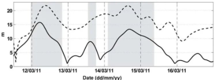
Figure 7. Estimates of the surface (continuous line) and bottom
(dashed line) Ekman depths (m). The gray patches show the periods where the sum of the surface and bottom Ekman depths exceeded 24 m (the water depth at station A2). The date indicates 00:00 UTC.
the storm; Grifoll et al., 2012). TheNvalues are estimated to be 0.03 s−1for the surface layer and 0.005 s−1for the bottom layer. The transient nature of the storm will cause some dif-ferences in the level of stratification, especially in the surface layer, but the relative size of the terms will remain mostly un-changed. Periods with less energetic wind conditions exhibit smaller wind stress; therefore, the relative importance of the Coriolis term increases at 24 m (Grifoll et al., 2012). Our re-sults show that the boundary layers overlapped most of the time during the storm event (Fig. 7). Even though the appli-cability of Eq. (9) has been questioned for areas influenced by freshwater discharge (Garvine, 2004; Dzwonkowski et al., 2014), the calculated Ekman layer depths are consistent with the importance of the frictional terms in the along-shelf dy-namics.
4.3 Cross-shelf variability of the along-shelf momentum terms
The cross-shelf variability of the along-shelf momentum is investigated with the help of the momentum terms calcu-lated at 50 m water depth. The frictional adjustment time, as observed through the evolution of the momentum terms at 50 m, exhibited a 4 h lag when compared with the fric-tional adjustment time at 24 m (Sect. 4.1), likely caused by the time delay in the vertical transfer of momentum. The linear drag coefficient is calculated following the same approach as for the analysis at 24 m, now adjusting the PGFRACCE+COR+FRIC term (without advection terms) to the observed value (PGFO) for the first peak of the storm. The resulting value,r=7.3×10⁻⁴m s−1, is close to the value ofrfor the inner shelf (8.5×10⁻⁴m s−1). This supports our conclusion that, during the first storm peak, the along-shelf momentum balance was controlled by the combination of lo-cal acceleration, Coriolis and friction, while the advective, Coriolis and radiation stress terms played a secondary role.
The relative ratio of the fluctuations (standard deviations) in the acceleration and wind stress terms,ρ0H ∂v/∂t¯
τys
Figure 8.(Top panel) cross-shelf transect of the frictional adjustment times for several along-shelf wind stresses(τ )together with the inertial
time off the city of Barcelona (18.15 h, grey solid line). The cross-shelf variation of the frictional adjustment time (computed following Eq. 8) is shown for storm peak conditions (red line) and averaged storm conditions (blue line). The two dotted lines correspond to wind stresses such that the frictional and inertial times become equal at 24 m (t24) and 50 m (t50) water depth. (Bottom panel) the location of the inertial,
frictional and transition zones for the peak and mean storm conditions. The ADCP locations at 24 m and 50 m are indicated with black and blue triangles, respectively.
and Fewings, 2012): in the Middle Atlantic Bight, around 0.3 and 0.5 at 25 and 50 m, respectively; and in the West Florida Shelf, 0.5 and 1 for 25 and 50 m, respectively. The larger val-ues found in the Catalan shelf are ascribed to the enhanced acceleration during the storm.
The size of the Coriolis term at 50 m increases in compar-ison to the size of this term estimated at 24 m water depth. The standard deviation of the Coriolis term also increases offshore, from 9.6×10⁻⁷m s−2at 24 m to 1.5×10⁻⁶m s−2
at 50 m. The ratio of the fluctuations between the Coriolis and wind stress terms,ρ0Hfu¯
τys
, increased from 0.3 at 24 m to 1.3 at 50 m water depth. Lentz and Fewings (2012) pre-sented ratios around 0.4 for the Middle Atlantic Bight and West Florida Shelf at 25 m, and between 2 and 3 at 50 m depth.
The increasing/decreasing importance of the Coriolis/bottom-frictional terms responds to a switch towards the geostrophic balance, typical in the transition from the inner to the mid-shelf. With increasing depth, the frictional effects decrease in the along-shelf momentum balance. Lee et al. (1984) observed that the Coriolis term doubled from 28 to 75 m water depth in the South Atlantic Bight (USA), with progressively smaller frictional terms. At
the start of our study period (11 March 2011, Fig. 5), the 50 m water depth Coriolis term was larger than the other terms, suggesting a geostrophic balance during the calm period.
During the storm period, the PGFRACCE+COR+FRIC term at 50 m is moderately correlated with the Coriolis term (R=0.55 with 95 % confidence level). This correlation sug-gests that the dynamic response at 50 m includes a large geostrophic component, of greater relevance than at 24 m, where the PGFR is less correlated with Coriolis (R=0.33 with 95 % confidence level). However, the acceleration and frictional terms, and likely the non-linear terms, also play an important role at 50 m water depth during the storm; for example, the acceleration terms at 24 and 50 m are also mod-erately correlated (R=0.64 with 95 % confidence level). Michaud et al. (2013), from observations in the Gulf of Lion (275 km north of our study area, Fig. 1) at 65 m depth, also emphasized the importance of the wind-induced geostrophic currents during a storm.
storm (surface stress τ=0.25 Pa), the frictional and iner-tial times are equal for water depths of 94 m; for the aver-age stress of the storm (surface stressτ =0.12 Pa) this hap-pens for water depths of 64 m. Thus, the frictional effects dominated for depths up to around 60 m, causing our cur-rent meters to be located in regions controlled by inner-shelf dynamics during the entire storm. For the frictional and in-ertial times to be the same, the wind stress would have to be 0.075 Pa at 50 m and 0.02 Pa at 24 m. Therefore, the Coriolis term is relatively not important at 24 m except for very low surface stresses, such as during the calm period between the two storm pulses (0.02 Pa); during those times other terms, like the pressure-gradient force, will dominate the along-shelf momentum balance (Grifoll et al., 2013).
5 Conclusions and final remarks
We have assessed the effects of the passage of a storm over the inner Catalan shelf (NW Mediterranean Sea) on the along-shelf momentum balance. At 24 m water depth, a primary momentum balance between acceleration, pressure-gradient and frictional forces (surface and bottom) is estab-lished. The Coriolis and the wave-induced momentum terms play a second-order role in the momentum balance. Our es-timates for the frictional adjustment time and Ekman depth confirm the prevalence of the frictional response of the flow at 24 m. The increasing importance of Coriolis at 50 m cor-responds to a shift towards the geostrophic behavior, charac-terizing the transition from the inner to the mid-shelf.
The storm (12–15 March 2011) had two separate wind peaks that caused currents with some similarities but also important differences. The main similarity was the local re-sponse to wind forcing, with the along-shelf flow (towards the southwest) accelerating to a maximum shortly after the wind peak, at a time when the joint effect of bottom stress and a northeastward pressure-gradient force (arising from down-wind water set up) compensated for the decreasing down-wind stress. Such a response was more obvious during the first peak (13 March), as the system started from a condition of weak along-shelf flow. During the relatively calm period be-tween both wind peaks (14 March), the pressure-gradient force turned toward the southwest and the flow remained in that direction. During this period, the winds were weakly on-shore, likely setting a cross-shelf geostrophic balance. By the end of the calm period, and lasting through the second wind peak (15 March), the momentum balance was charac-terized by the appearance of fluctuations with both super-inertial (12–16 h) and sub-super-inertial (1–2 days) periods. During the second wind peak, the temporal sequence of increased ac-celeration followed by opposing bottom stress and pressure gradient reoccurred, but with the along-shelf flow largely in-fluenced by the sub-inertial (likely topographic) waves, with velocity amplitudes as large as 0.3 m s−1. These waves re-mained active even when the second wind peak had ended.
In our analysis, we have focused on the shelf response to a single twin storm, where extensive observational data were available. However, northeasterly energetic wind events are common during spring and fall in the Catalan shelf; there-fore, similar events are expected on a yearly basis. The ex-trapolation of our results to other shelves depends on phys-ical variables such as stratification, river discharge and re-mote sea-level forcing. In relatively low-energy shelves, such as the Catalan shelf, it is plausible that two-peak storms be commonly characterized by a sequence of a linear response followed by a subsequent non-linear behavior.
was presented by Csanady (1981), based on the transport mo-mentum equation in the along-shelf direction:
∂V
∂t +f U= −gH ∂η ∂y+u
∗2−τyb
ρ , (A1)
where the transport is
U= 0
Z
−H
udz, (A2a)
V = 0
Z
−H
vdz, (A2b)
and the frictional velocity is given by
u∗= rτ
ys
ρ . (A3)
Under the assumption that the depth distribution is only a function of the cross-shelf coordinate, we neglect the along-shelf pressure gradients. Also, the coastal constraint near the coast impliesU=0. These conditions lead a frictional balance between the acceleration and the wind and bottom stresses:
∂V ∂t =u
∗2−τyb
ρ . (A4)
The bottom stress was parameterized by Csanady (1981) using a quadratic drag law equation as a function of the depth-averaged current (V /H):
τyb ρ =Cda
V H
2
. (A5)
Integrating, the solution for the along-shelf transport fol-lows an exponential equation
V = u ∗H
√ Cda
1−exp −2u∗t√Cda/H 1+exp −2u∗t√Cda/H
!
, (A6)
with ane-folding timescale of
tf = H
2qτysCda
ρ
. (A7)
Alternatively, we may consider the bottom frictional term to depend linearly on the depth-averaged current:
τyb ρ =r
V H
. (A8)
where thee-folding timescale is H /r, as expected accord-ing to the lineal parameterization of the bottom stress in Eq. (2). Linear and quadratic derived frictional time expres-sions have the same physical meaning, withe-folding times proportional to the water depth and inversely proportional to bottom stress parameter (r or Cda). For the linear and quadratic formulations, at long times the depth-averaged ve-locities tend asymptotically to √u∗
Cda and
u∗2
r , respectively, which are the velocities required for bottom stress to balance the wind stress.
Appendix B: Topographic waves over the continental shelf
Here, we follow Csanady (1982, Sect. 4.5) to estimate the size of the coastal propagating anomalies. We look at the non-forced propagation of a sea surface perturbation, with elevationη, generated at some earlier time in some upstream location along the coast. We keep the same coordinate con-vention as in the main text, with (x, y), respectively directed cross shelf and along shelf (positive offshore and to the north-east). Following Grifoll et al. (2013), we let the dominant terms in the cross-shelf direction to be in geostrophic bal-ance. Hence, the linearized depth-averaged momentum- and mass-conservation equations for non-stratified and friction-less conditions are (dropping overbars):
−f v= −g∂η
∂x, (B1)
∂ (vH )
∂t +f uH = −gH ∂η
∂y, (B2)
∂ (uH )
∂x +
∂ (vH ) ∂y = −
∂η
∂t. (B3)
Let us idealize our coastal ocean as having the water depth independent of the along-shelf distance,H=H (x). Taking the curl of the momentum equations and using the mass-conservation equation leads to the following vorticity equa-tion (constantf condition)
∂2(vH ) ∂t ∂x −f
∂η
∂t = −g dH
dx ∂η
∂y. (B4)
In the cross-shelf direction the change in water depth is much greater than the change in surface elevation (the equiv-alent of assuming the rigid lid approximation for the mass-conservation equation), i.e., ∂(vH )
∂x ≫∂η/∂t. Hence, we may safely neglect the second term in the left-hand side of Eq. (B4) so that, using Eq. (B1), we get
∂2 ∂t ∂x H∂η ∂x
+fdH dx
∂η
We need two boundary conditions to solve this equation. The first one comes from the condition of no-normal flow at the coast; from Eq. (B2), and with the help of Eq. (B1), we obtain
∂2η ∂t ∂x +f
∂η
∂y =0, at x=0. (B6)
The second condition may be simply specified from the requirement of a finite-size perturbation; from Eq. (B1) this is equivalent to setting that far enough from the coast the elevation of the perturbation tends to zero:
∂η
∂x =0 at x=Lx. (B7)
Here, we chooseLxto be the width of the continental shelf (i.e., the offshore extent of the perturbation is limited by the width of the coastal band). For our study, we take this to be the characteristic width of the continental shelf north of Barcelona, or about 40 km.
The solution of Eq. (B5) subject to the boundary condi-tions (B6) and (B7) is obtained through separation of vari-ables,η (x, y, t )=φ (y, t ) χ (x). The equation forφ (y, t ) be-comes
∂φ ∂t −ci
∂φ
∂y =0, (B8)
whereciis the separating constant. The general solution cor-responds to a wave propagating in the negativeydirection (in our case, towards the southwest),φ (y+cit ), showing thatci corresponds to the phase speed of the traveling perturbation. Following Csanady (1982), let the water depth be a linear function of the cross-shelf distance,H (x)=xH0/Lx≡sx, wheresis the slope. The equation forχ (x)becomes
ξd 2χ
dξ2 + dχ
dξ +χ=0, (B9)
whereξ ≡f x/ci. The boundary condition at the coast be-comes ci
f
dχ
dx+χ=0, and the condition atx=Lx turns into dχdx =0. Equation (B9) together with these boundary conditions is an eigenvalue problem, with different solu-tions for a discrete number of positive ci values. The so-lution that satisfies the boundary condition at the coast is χ=AJ0 2ξ1/2, whereJ0 is a Bessel function of order 0, andAis a constant. The boundary condition atx=Lxsets the possiblecivalues, those that satisfyJ12(f l/ci)1/2
=0,
whereJ1is a Bessel function of order 1. The faster wave cor-responds to c1=f Lx/3.67, having the simplest structure: maximum velocity at the coast that decreases to zero atLx.
From Eq. (B1), the along-shelf velocity is v= −(gAφ) /(cif x)1/2J1
2qf x ci
. The
maxi-mum velocity takes place at the coast, given by v= −(gAφ)c
1 = −(3.67gAφ) / (f Lx), its magnitude
de-pending on the elevation Aφ at the coast. In Fig. 3e, we
see changes in elevation as large as 0.05 m taking place on timescales of 1–1.5 days, which would represent velocities of about 0.3 m s−1, which is in fair agreement with the observed oscillations (Fig. 3b).
The periodicity of these perturbations depends on the size of the region where they are generated, which sets the along-shelf wavenumber k=2π/Ly. The shortest period corre-sponds to the fastest propagating perturbations, which are also the ones that result in the largest along-shelf velocities; it turns out to beT ≡2πω ≡(c2π
1k)= 3.67Ly
f Lx . If we chooseLy
to be 120 km, or about the size of the domain with maximum gradients in sea-level pressure (and hence maximum winds) (Fig. 2), we getLy/Lx∼=3 and the period is about 32 h. This number is to be taken only as a very rough estimate but yet it suggests that some of the energy in the spectra analyses (Fig. 6), in the 1–2 day band, comes from propagating topo-graphic waves.
Acknowledgements. This work was supported by DARDO
(ENE2012-38772-C02-02), Rises-AM (GA603396), Plan-Wave (CTM2013-45141-R) and ICoast project (Echo/SUB/2013/661009). We would like to thank Joan Puigde-fàbregas, Jordi Cateura and Joaquim Sospedra (LIM-UPC, Barcelona, Spain) for the data acquisition campaign. The authors thank Alexis Beudin (USGS, Woods Hole, USA) and Ken Brink (WHOI, Woods Hole, USA) for a number of useful suggestions. We are also very grateful to our reviewers, Vlado Malaˇciˇc and one anonymous oceanographer, for their ideas; Vlado Malaˇciˇc raised the issue of the potential relevance of coastal waves, which meant a substantial reanalysis of our velocity data and a reinter-pretation of our results. Finally, we are pleased to acknowledge Gabriel Csanady and Steve Lentz, as their seminal studies on the circulation of the coastal ocean have been a source of inspiration to our work.
Edited by: S. Carniel
References
Booij, N., Ris, R. C. and Holthuijsen, L. H.: A third-generation wave model for coastal regions: 1. Model description and valida-tion, J. Geophys. Res., 104, 7649, doi:10.1029/98JC02622, 1999. Brink, K. H. and Chapman, D. C.: Programs for Computing Prop-erties of Coastal Trapped waves and Wind-driven Motions over the Continental Shelf and Slope, Woods Hole Oceanographic In-stitute Tech. Rep. WHOI 85-17, 99 pp., 1985.
Csanady, G. T.: Circulation in the coastal ocean, Adv. Geophys., 23, 101–183, 1981.
Csanady, G. T.: Circulation in the coastal ocean, D. Reidel Publish-ing Company, 279 pp., Dordretch, Holland, 1982.
inner shelf off New Jersey, J. Mar. Res., 62, 337–371, 2004. Gill, A. E.: Atmosphere-ocean dynamics, Academic Press, London,
England, 662 pp., 1982.
Grifoll, M., Aretxabaleta, A. L., Espino, M., and Warner, J. C.: Along-shelf current variability on the Catalan inner-shelf (NW Mediterranean), J. Geophys. Res., 117, 1–14, 2012.
Grifoll, M., Aretxabaleta, A. L., Pelegrí, J. L., Espino, M., Warner, J. C., and Sánchez-Arcilla, A.: Seasonal circulation over the Catalan inner-shelf (northwest Mediterranean Sea), J. Geophys. Res. Ocean., 118, 5844–5857, 2013.
Grifoll, M., Gracia, V., Aretxabaleta, A. L., Guillén, J., Espino, M., and Warner, J. C.: Formation of fine sediment deposit from a flash flood river in the Mediterranean Sea, J. Geophys. Res. Ocean., 119, 5837–5853, 2014.
Hickey, B. M.: The Fluctuating Longshore Pressure Gradient on the Pacific Northwest Shelf: A Dynamical Analysis, J. Phys. Oceanogr., 14, 276–293, 1984.
Jordi, A., Orfila, A., Basterretxea, G., and Tintoré, J.: Coastal trapped waves in the northwestern Mediterranean, Cont. Shelf. Res., 25, 185–196, 2005.
Kirincich, A. R., Barth, J. A.: Alongshelf Variability of Inner-Shelf Circulation along the Central Oregon Coast during Summer, J. Phys. Oceanogr., 39, 1380–1398, 2009.
Kohut, J. T., Glenn, S. M., and Paduan, J. D.: Inner shelf re-sponse to Tropical Storm Floyd, J. Geophys. Res., 111, C09S91, doi:10.1029/2003JC002173, 2006.
Kundu, P. K. and Thomson, J. P.: Inertial oscillations due to a mov-ing front, J. Phys. Oceanogr., 15, 1076–1084, 1985.
Kundu, P. K., Chao, S., and McCreary, J. P.: Transitient coastal cur-rents and inertia-gravity waves, Deep-Sea Res., 30, 10A, 1059– 1082, 1983.
Large, W. G. and Pond, S.: Open Ocean Momentum Flux Measure-ments in Moderate to Strong Winds, J. Phys. Oceanogr., 11, 324– 336, 1981.
Lee, T. N., Ho, W. J., Kourafalou, V., and Wang, J. D.: Circulation On the Continental Shelf of the Southeastern United States, Part I: Subtidal Response to Wind and Gulf Stream Forcing During Winter, J. Phys. Oceanogr., 14, 1001–1012, 1984.
Geophys. Res., 104, 18205–18226, 1999.
Lentz, S. J. and Fewings, M. R.: The Wind- and Wave-Driven Inner-Shelf Circulation, Ann. Rev. Mar. Sci., 4, 317–343, 2012. Lentz, S. J. and Winant, C. D.: Subinertial Currents on the Southern
Califoinia Shelf, J. Phys. Oceanogr., 16, 1737–1750, 1986. Longuet-Higgins, M. and Stewart, R.: Radiation stresses in water
waves; a physical discussion, with applications, Deep-Sea Res., 11, 529–562, 1964.
Maza, M., Voulgaris, G., and Subrahmanyam, B.: Subtidal in-ner shelf currents off Cartagena de Indias, Caribbean coast of Colombia, Geophys. Res. Lett., 33, 1–5, 2006.
Michaud, H., Marsaleix, P., Leredde, Y., Estournel, C., Bourrin, F., Lyard, F., Mayet, C., and Ardhuin, F.: Three-dimensional mod-elling of wave-induced current from the surf zone to the inner shelf, Ocean Sci., 8, 657–681, 2012.
Michaud, H., Leredde, Y., Estournel, C., Berthebaud, É., and Marsaleix, P.: Modelling and in-situ measurements of intense currents during a winter storm in the Gulf of Aigues-Mortes (NW Mediterranean Sea), Comptes Rendus Geosci., 345, 361– 372, 2013.
Salat, J., Tintore, J., Font, J., Wang, D.-P., and Vieira, M.: Near-Inertial Motion on the Shelf-Slope Front off Northeast Spain, J. Geophys. Res., 97, 7277–7281, 1992.
Scott, J. T. and Csanady, G. T.: Nearshore Currents off Long Island, J. Geophys. Res., 81, 5401–5409, 1976.
Shearman, R. K.: Observations of near-inertial current variabil-ity on the New England shelf, J. Geophys. Res., 110, C02012, doi:10.1029/2004JC002341, 2005.
Tintoré, J., Wang, D.-P., García, E., and Viúdez, A.: Near-Inertial Motion in the coastal ocean, J. Mar. Syst., 6, 301–312, 1995. Weatherly, G. and Martin, P.: On the structure and dynamics of the
oceanic bottom boundary layer, J. Phys. Oceanogr., 8, 557–570, 1978.