Lagrangian transport modelling for CO<sub>2</sub> using two different biosphere models

(1)

ACPD

8, 4117–4154, 2008

Lagrangian transport modelling for CO₂

G. Pieterse et al.

Title Page

Abstract Introduction

Conclusions References

Tables Figures

◭ ◮

Back Close

Full Screen / Esc

Printer-friendly Version

Interactive Discussion

EGU

Atmos. Chem. Phys. Discuss., 8, 4117–4154, 2008 www.atmos-chem-phys-discuss.net/8/4117/2008/ © Author(s) 2008. This work is licensed

under a Creative Commons License.

Atmospheric Chemistry and Physics Discussions

Lagrangian transport modelling for CO

₂

using two di

_ff

erent biosphere models

G. Pieterse1,2, A. T. Vermeulen1, I. T. Baker3, and A. S. Denning3

1

Energy research Centre of the Netherlands, Petten, The Netherlands

2

Institute for Marine and Atmospheric Research Utrecht, Utrecht, The Netherlands

3

Colorado State University, Fort Collins, USA

Received: 4 December 2007 – Accepted: 11 January 2008 – Published: 28 February 2008

(2)

ACPD

8, 4117–4154, 2008

G. Pieterse et al.

Title Page

Tables Figures

◭ ◮

Back Close

Full Screen / Esc

EGU

Abstract

In this work, the performance of the Framework for Atmosphere-Canopy Exchange

Modelling (FACEM: Pieterse et al.,2007) coupled to a Lagrangian atmospheric

trans-port model is evaluated for carbon dioxide. Before incorporating FACEM into the

La-grangian COMET model (Vermeulen et al.,2006), its performance for the European

5

domain is compared with the Simple Biosphere model (SiB3: Sellers et al., 1996).

Overall, FACEM is well correlated to SiB3 (R2_≥₀._{60), but shows less variability for}

re-gions with predominantly bare soil. There is no significant overall bias between the models except for the winter conditions and in general for the Iberian peninsula. When coupled to the COMET transport model, both biosphere models yield similar

correla-10

tions (R2_≥₀._{60) and bias relative to the 1-hourly concentration measurements for the}

year 2002, performed at three different sites in Europe; Cabauw (Netherlands),

Hegy-hatsal (Hungary) and Mace Head (Ireland). The overall results indicate that FACEM is comparable to SiB3 in terms of its applicability for atmospheric modelling studies.

1 Introduction

15

A significant part of the work performed within the field of environmental research is

currently focussing on the development of climate models (Randall et al.,2007). The

goal of the scientific work on this subject is to produce realistic predictions for the short and long term response of the global climate system on the increasing carbon

dioxide concentration (IPCC,2007). The most challenging part is that a large number of

20

physical, chemical and/or biological processes occurring over a large range of temporal

and spatial scales have a significant effect and therefore must be incorporated in these

models for adequate predictions.

Of high importance is an appropriate scheme that describes the short and long term biospheric response to climatic drivers such as solar radiation, precipitation, air

tem-25

(3)

ACPD

8, 4117–4154, 2008

G. Pieterse et al.

Title Page

Tables Figures

◭ ◮

Back Close

Full Screen / Esc

EGU

insight into the spatial and temporal impact of the main processes determining the magnitude and timing of the response of the terrestrial biosphere to the main driving parameters. For this purpose, numerous advanced physiological, flux and concentra-tion measurements (laboratory scale, ground based, airborne or remote sensing), are currently performed or developed. Realisation of such measurements is still

accom-5

panied with technological and methodological challenges, of which accuracy, precision and inter comparability are the most important limiting factors.

During the last 30 years a world wide network of measurement sites has been

es-tablished to monitor the global trend of CO2and other greenhouse gases (

Globalview-CO2, 2005). The sites contributing to this network are located at remote regions to

10

reduce the local influence of anthropogenic and biogenic contributions compared to the much slower varying global background concentrations. Highly accurate calibra-tion methods and data qualificacalibra-tion routines are used to ensure optimal data quality (World Meteorological Organisation,2007). These procedures make the data obtained from these sites very valuable for longer term global climate studies. However, these

15

measurements are by design less suitable for continental greenhouse budget investiga-tions as the source and sink information is too diluted at these sites. Therefore, recent

projects, e.g. CarboEurope IP (http://www.carboeurope.org), the project for

Continu-ous HIgh-precisiOn Tall Tower Observations (CHIOTTO: http://www.chiotto.org), and

the North American Carbon Program (NACP:http://www.nacarbon.org/nacp), have

fo-20

cussed on developing networks of continental sites employed especially to monitor

continental CO2 concentrations. These sites are generally situated in regions highly

influenced by anthropogenic as well as biospheric activity. Hence, the measurements obtained from these sites are complex mixed signals with large and (sometimes) com-pensating contributions from biospheric and anthropogenic activity. Adequately

inter-25

preting these signals and quantifying the biospheric and anthropogenic contributions to these signals requires the use of accurate high resolution atmospheric transport models.

(4)

ACPD

8, 4117–4154, 2008

G. Pieterse et al.

Title Page

Tables Figures

◭ ◮

Back Close

Full Screen / Esc

EGU

such atmospheric transport models difficult. This asks for the concurrent development

of sophisticated biosphere models that are able to accurately describe the processes that take place in the biosphere. The approach that is chosen for this study however is partly moving away from this growing complexity for reasons explained below.

An important fact is that most biospheric and atmospheric model studies are almost

5

by definition under determined, i.e. that there are not enough measurements available to solve for all unknowns in a certain problem. As a general rule, a certain minimum number of processes that capture the most important features of a certain complex system need to be included in a model. Adding more processes in an attempt to cap-ture even more feacap-tures does not necessarily lead to improved accuracy, even though

10

these newly added processes can be conceptually correct and their inclusion seems justifiable. Namely, along with each new process, a number of new parameters are introduced. An increasing amount of poorly determined parameters will add to the un-certainty and it is therefore important to realise that including more complexity can lead to loss of accuracy.

15

This work illustrates the applicability of a new biosphere model, the Framework for

Atmosphere Canopy Exchange Modelling (FACEM: Pieterse et al., 2007), to

atmo-spheric transport modelling of CO2. For this purpose, FACEM was coupled to the

La-grangian CO2and Methane Transport (COMET) model (Vermeulen et al.,1999,2006).

Both models were developed keeping the above described “uncertainty accumulation”

20

in mind and only contain the crucial processes required to capture the most impor-tant features of atmospheric transport and the biospheric processes responsible for

the exchange of CO₂ between the biosphere and atmosphere. This design limits the

application of both models to regions without complex orographic features. Section2

starts with a brief description of the overall model framework and the chosen method

25

(5)

ACPD

8, 4117–4154, 2008

G. Pieterse et al.

Title Page

Tables Figures

◭ ◮

Back Close

Full Screen / Esc

EGU

2 Methods

Before addressing the full model framework, the model is evaluated by a European scale comparison between FACEM and the more sophisticated Simple Biosphere

model (SiB: Sellers et al., 1996) that provides global biospheric CO₂ flux estimates.

Thereafter, both biosphere models are coupled to COMET and the overall

perfor-5

mance is evaluated in a comparison with 1-hourly concentration measurements from

three different European continuous measurement sites for the year 2002. Both model

frameworks are evaluated with respect to their capability to predict the concentrations measured at these sites.

2.1 Used models and additional data

10

2.1.1 Biosphere models

FACEM is a Soil-Vegetation-Atmosphere-Transfer (SVAT) model that calculates Gross Primary Productivity (GPP), Net Primary Productivity (NPP) and Net Ecosystem

Pro-ductivity (NEP). The GPP accounts only for the uptake of CO2due to photosynthesis.

NPP also incorporates the release of CO2 due to biomass growth and maintenance

15

(i.e. autotrophic respiration). NEP accounts for all processes including the release of

CO2 from the soil carbon pools due to microbe activity (i.e. heterotrophic respiration).

The sum of autotrophic and heterotrophic respiration is called total respiration. With FACEM, these quantities can be calculated on a 1-hourly time resolution and a spatial

resolution of 0.₅◦_×₀.₅◦_{for the European domain.}

20

Within FACEM, the exchange of CO2between the biosphere and the atmosphere is

modelled using a mechanical multi layer model for photosynthesis (Berry and Farquhar,

1978;Collatz et al.,1991;Wu et al.,2003). A passive membrane transport model is used to calculate the leaf cuticle resistance. The photosynthesis scheme provides a full description of the stomatal resistance of the leafs coupled to the biochemical

mech-25

(6)

environ-ACPD

8, 4117–4154, 2008

G. Pieterse et al.

Title Page

Tables Figures

◭ ◮

Back Close

Full Screen / Esc

EGU

mental conditions. Compared to the traditional single layer approach, the multi layer approach allows for a more adequate treatment of the non-linear transport of radiation through the canopy and a more accurate calculation of the boundary layer resistance. Autotrophic respiration is estimated by a scheme adopted from an algorithm used to

produce MODIS NPP products (Heinsch et al.,2003). Growth respiration is calculated

5

following the approach introduced byKnorr(2000). Finally, heterotrophic respiration is

calculated using the approach introduced byIto and Oikawa(2000) andAurora(2003).

A more detailed description of FACEM was previously given byPieterse et al.(2007).

The SiB model was described extensively in (Sellers et al., 1996; Denning et al.,

1996;Baker et al.,2003;Vidale and Stoekli,2005;Baker et al.,2006) and yields global

10

1-hourly fluxes for GPP and total respiration on a 1.₀◦_×₁.₀◦ _{resolution (}_{Baker et al.}_,

2007). Conceptually, FACEM and SiB differ significantly. FACEM was mainly designed

for provision of reasonable initial estimates for forward and inverse modelling of the

current exchange of CO₂ between the biosphere and atmosphere and makes use of

available measurements whenever the alternative, a mechanical model, is considered

15

to be a source of larger uncertainty. SiB was originally designed for calculating the exchange of energy, mass and momentum from the terrestrial biosphere to the lower boundary of atmospheric circulation models. For this purpose and to address also

more detailed ecological questions, inclusion of the exchange of CO2 between the

biosphere and atmosphere was vital. Because CO₂is an important driver for global

cli-20

mate (IPCC,2007), it is important to keep track of the present, past and future carbon

budgets for the atmosphere, vegetation as well as for the soil. Since more and more measurements have become available recently, the latest versions of the SiB model (resulting in SiB3) have been optimised in its ability to reproduce these measurements. It is for this reason that the SiB3 model is considered an excellent benchmark to

vali-25

(7)

ACPD

8, 4117–4154, 2008

G. Pieterse et al.

Title Page

Tables Figures

◭ ◮

Back Close

Full Screen / Esc

EGU

2.2 Atmospheric transport model

A detailed theoretical treatment and validation of the Lagrangian CO2 and Methane

Transport (COMET) model was previously given byVermeulen et al.(1999,2006). In

short, the COMET model approximates the transport of any chemically inert gaseous atmospheric constituent towards a measurement site by a closed 2-layer box moving

5

along a Lagrangian trajectory that ends at the measurement site. The trajectories are

obtained using the Flextra model (Stohl et al.,1995;Stohl and Seibert, 1998) which

uses the same European Centre of Medium range Weather Forecast (ECMWF) data that is used by the FACEM model. While moving along the trajectory, the box

accumu-lates and releases tracer, in this case CO₂, from and to the surface sources and sinks.

10

The height of the interface between the two layers in the box changes according to the calculated Planetary Boundary Layer (PBL) height. This models the exchange of air between the lower well-mixed and the upper reservoir layer. By initialising the trations at the start of each trajectory to the spatially interpolated background

concen-tration measurement data provided by Globalview-CO2 (Globalview-CO2, 2005), and

15

by employing the estimates for the spatial and temporal distribution of sources and

sinks for CO2, the COMET model provides means to calculate 1-hourly averaged CO2

concentrations for any given measurement site within the well-mixed PBL. The results shown in this paper will focus on the domain of western Europe.

2.3 Used additional data sets

20

A global data set (Takahashi et al., 2002) was used to provide estimates for the

ex-change of carbon dioxide between the atmosphere and the ocean. Finally, the Edgar

Fast Track emission inventory (Olivier et al., 2005) was used to provide the

(8)

ACPD

8, 4117–4154, 2008

G. Pieterse et al.

Title Page

Tables Figures

◭ ◮

Back Close

Full Screen / Esc

EGU

3 Model evaluation

In this section, FACEM and SiB3 are first compared for the European domain. There-after, both models are coupled to COMET and the resulting modelled well-mixed layer concentrations are compared to the measurements at Cabauw, Hegygatsal and Mace Head.

5

3.1 Flux model evaluation

The grid based evaluation described in this section required spatial matching of the

re-sults because FACEM and SiB3 are run at di_fferent spatial resolutions (see Sect.2.1.1)

and by default use different land masks. Therefore, the land mask of the SiB3 model

was applied to the FACEM model results after completing the calculations using the

10

FACEM land mask. Grid cells for which model results were available from only one of the two models, were excluded. SiB3 provides results for GPP and total respiration. Therefore, we chose to compare GPP and NEP.

3.1.1 Gross Primary Productivity

In Fig.1, the spatial correlation (R2_{) between the modelled GPP fluxes, the relative}

dif-15

ference in the standard deviation (∆σ_{) and relative bias between the modelled GPP}

fluxes are shown for the spring (a–c), summer (d–f), autumn (g–i) and winter (j–l) season. The latter two quantities are referenced to the SiB3 model results and are expressed in relative deviation percentages.

It is clear that both models correlate well (R2_≥₀._{60) for the spring season, except for}

20

the Northern part of Scandinavia and for the Iberian peninsula. For high latitudes, the

Leaf Area Index (LAI) product (Knyazikhin et al.,1999) used by FACEM is scarce and

less accurate. For these regions, this could well be an explanation for the discrepancy between both models. In the central part of the Iberian peninsula GPP is low and

therefore small differences between both models have a large effect on correlation and

(9)

ACPD

8, 4117–4154, 2008

G. Pieterse et al.

Title Page

Tables Figures

◭ ◮

Back Close

Full Screen / Esc

EGU

relative differences between variability and bias. This is also the case for the winter

season when GPP is low all over Europe. Additionally, the land use classes for the

Iberian peninsula are different for both models. FACEM assigns C3 crops and grasses

to this region whereas SiB3 uses broad leaf deciduous trees over wheat. The use of

di_fferent land use classes is very likely the cause for the observed di_fferences between

5

the model results for the Iberian Peninsula.

For the United Kingdom, FACEM yields significantly less variable and lower average GPP. FACEM uses interpolated meteorological data to calculate the fluxes at a

resolu-tion of 0.₅◦_×₀.₅◦_{. The SiB3 calculations were performed at a coarser spatial resolution}

and the fluxes are provided at a resolution of 1.₀◦_×₁.₀◦_{. This di}_ff_{erence can cause}

10

significant di_fferences for locations with mixed oceanic and continental meteorological

conditions, e.g. the United Kingdom or Ireland. Section 3.2.3 will discuss this

phe-nomenon in a comparison with measurements performed at the Mace Head station.

In all, the two models correlate reasonably well (R2_≥₀._{50) for the Summer season,}

with again the exception of the Iberian peninsula. An anomaly of enhanced variability

15

and positive bias occurs in the Southern part of France during Summer and Autumn. The Available Soil Water (ASW) budget implemented in FACEM indicates a relatively high ASW content for this region but the ASW is still in the optimal range for

photosyn-thesis. In Fig. 2, the seasonally averaged results of both models are compared with

the seasonally averaged MODIS GPP product (Heinsch et al.,2003). For the spring,

20

summer and autumn season both FACEM and MODIS show enhanced GPP for the Southern part of France. It is clear that, overall, FACEM and the MODIS produce very similar spatial patterns. This not surprising because FACEM makes use of the MODIS

LAI product to calculate GPP whereas in SiB3 Normalised Difference Vegetation

In-dex (NVDI) data from the Advanced Very High Resolution Radiometer (AVHRR: Teillet

25

et al.,2000) is used. It is therefore likely that the differences between both models can

(10)

ACPD

8, 4117–4154, 2008

G. Pieterse et al.

Title Page

Tables Figures

◭ ◮

Back Close

Full Screen / Esc

EGU

3.1.2 Net Ecosystem Productivity

Figure3 shows the correlation (R2_{), relative di}_ff_{erence in the standard deviation (}_∆σ₎

and the relative bias between the modelled NEP fluxes for the spring (a–c), summer (d– f), autumn (g–i) and winter (j–l) season. Again, the latter two quantities are referenced to the SiB3 model results and are expressed in deviation percentages.

5

The figure shows similar but more pronounced discrepancies as those found for the

GPP fluxes in the previous section. The differences are again largest for the Iberian

peninsula, the higher latitudes and the United Kingdom. In the North-Eastern part of Europe the average NEP, as predicted by FACEM, is larger by more than 80%. In the current version of FACEM, the autotrophic respiration model does not account

10

for snow cover or frost conditions. Adapting the soil respiration scheme in FACEM for winter conditions will most likely improve the performance. Furthermore, SiB3 is well equipped for predicting the diurnal and seasonal variability but is not designed to reproduce net sources and sinks. The magnitude of a net local source or sink at a certain location is small, generally in the order of 10% or less. An uncertainty in the

15

magnitude of this local source or sink will therefore not significantly affect the absolute

error in the calculated instantaneous flux (Denning et al.,1996). Therefore, SiB3 forces

annual NEP to zero and the respiration fluxes will on average exactly cancel the GPP fluxes. Both models agree well for the central part of Europe, which is the region of interest for the comparison in the following section.

20

3.2 Overall model evaluation

COMET model calculations were performed for the Cabauw tall tower site (Ulden and

Wieringa,1996;Beljaars and Bosveld,1997) in the Netherlands and the results were

compared with 1-hourly averaged PBL concentration measurements for the year 2002. The following six cases were considered for the evaluation:

25

(11)

ACPD

8, 4117–4154, 2008

G. Pieterse et al.

Title Page

Tables Figures

◭ ◮

Back Close

Full Screen / Esc

EGU

photosynthesis or primary productivity (case 2 and 5), autotrophic respiration (added in case 3) and heterotrophic respiration (added in case 4 and 6). Case 1 is the refer-ence case and gives insight in the magnitude of the contributions from anthropogenic sources and oceanic sinks, the latter of which was considered small compared to the anthropogenic contributions. The same procedure was repeated for the Hegyhatsal Tall

5

tower in Hungary (Hazpra,2006) and the Mace Head observatory in Ireland (Derwent

et al.,2002), also for the year 2002. The three sites are described in Table2.

3.2.1 The Cabauw tall tower

For the Cabauw tall tower, the results for the di_fferent cases are shown in Table3.

The results clearly indicate that incorporating the NEP as an estimate for the

10

biosphere-atmosphere exchange yields the best model-to-measurement correspon-dence, both in terms of correlation as well as in terms of variability and bias. This is valid for both FACEM as well as SIB3 and indicates good performance of all processes included in the FACEM and the SiB3 model, especially considering the completely

dif-ferent agreement for Case 2, measured by a poor correlation (R2₌_{0.35). Overall, the}

15

performance obtained using FACEM is comparable to the performance obtained using

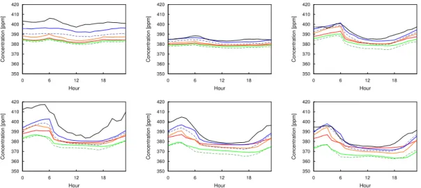
SiB3, also for day and night time conditions. In Fig. 4, the monthly averaged

diur-nal cycles of the modelled and measured sigdiur-nals are shown. All months have≥75%

valid data coverage except January (45%), April (9%), May (54%), August (64%) and December (0%).

20

The anthropogenic and oceanic contributions (solid red) add relatively little to the variability of the modelled signals, suggesting a larger influence of the local terrestrial biosphere on the measured variability than the local anthropogenic sources. For both

biosphere models, GPP is responsible for a large uptake of CO₂ (solid and dashed

green) during the spring and summer season. However, this uptake is compensated

25

by release of CO2 due to autotrophic and heterotrophic respiration, as illustrated by

(12)

model-ACPD

8, 4117–4154, 2008

G. Pieterse et al.

Title Page

Tables Figures

◭ ◮

Back Close

Full Screen / Esc

EGU

to-measurement performance. For the winter months, when respiration processes dominate the biospheric flux, the variability is well predicted by both biosphere

mod-els, however the model results show a stronger bias. As mentioned in Sect.2.2, the

transport model is initialised by measured background concentrations. An important limitation of this approach is that for cases where the used background concentration

5

(at the starting point of each trajectory) is not representative for the actual background concentration, a bias will be observed between the modelled and measured trations leading to lower modelled concentrations compared to the observed concen-trations. Such circumstances develop mainly in the winter season with flow conditions where continental air masses are transported from east to west, which is the case for

10

Cabauw.

It is striking to see how the modelled GPP signal is concealed by heterotrophic

res-piration. The uptakes of CO2 due to photosynthesis, that are clearly present in case 2

and 5 are barely discernible in the measured signals. This has an important conse-quence for the use of concentration measurements for estimating the carbon budget in

15

the influence area of this measurement site. It will be difficult, if not impossible, to

dis-sect the different contributions of the biosphere to the measurements using

concentra-tion measurements only. Considering the magnitude of the contributing and opposing signals and the uncertainties involved in the atmospheric transport modelling,

deter-mining the different contributions would very likely result in significant uncertainties.

20

However, it appears that determining the combined contributions of the anthropogenic sources and NEP is feasible, considering the good model-to-measurement correspon-dence represented by cases 4 and 6.

3.2.2 The Hegyhatsal tall tower

For the Hegyhatsal tall tower, the results for the different cases are shown in Table4.

25

A striking difference with the model performance for Cabauw can be seen here for

(13)

measure-ACPD

8, 4117–4154, 2008

G. Pieterse et al.

Title Page

Tables Figures

◭ ◮

Back Close

Full Screen / Esc

EGU

ments for the case when only fossil fuel sources are taken into account. Again, the NEP case results in the best model-to-measurement correspondence, both in terms of

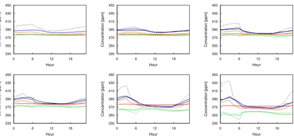
correlation as well as in variability and bias. In Fig. 5, the monthly averaged diurnal

cycles of the modelled and measured signals are shown. All months have≥75% valid

data coverage except January (0%), July (65%), August (14%) and September (41%).

5

From this figure, it can be seen that the contribution of fossil fuel emissions to the diurnal cycle are nearly negligible (red). The GPP (solid and dashed green) is clearly

responsible for a large uptake of CO₂ during spring and summer. Again, this uptake

is compensated by releases due to autotrophic and heterotrophic respiration (orange, solid and dashed blue). The model results using NEP fluxes from SiB3 (dashed blue)

10

overestimate the measurements. Assuming that SiB3 fluxes are correct, this leads to the conclusion that the nocturnal PBL height is underestimated for stable night time conditions. In the PBL scheme implemented in COMET, the PBL height is limited to a minimum height of 50m. It is plausible that more vertical mixing occurs due to local surface inhomogeneities than is predicted using the relatively coarse ECMWF data.

15

For this reason, the COMET model calculations were repeated using the SiB3 NEP estimates and using 100m as the lower limit for the nocturnal PBL height, resulting in a

significant improvement (R2₌₀._55,σ₌₁₃._{2 ppm, bias}₌_{–2.2 ppm) compared to Case 6}

in Table4(R2₌₀._44,σ₌₂₃._{1 ppm, bias}₌_{3.5 ppm). It is also possible that the modelled}

heterotrophic respiration fluxes from SiB3 are too large for the region of influence of

20

the Hegyhatsal tower. As can be seen in Fig. 2, SiB3 tends to predict larger GPP in

Hungary than observed by MODIS, and therefore the heterotrophic respiration fluxes

are expected to be relatively high as well (see Sect.3.1.2. CO₂flux measurements are

required to determine whether (a combination of) both sources of error can explain the discrepancy but were not available for this study.

25

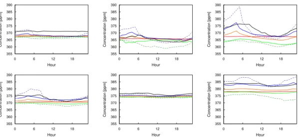
3.2.3 The Mace Head site

For the site at Mace Head, the results for the different cases are summarised in Table5.

(14)

ACPD

8, 4117–4154, 2008

G. Pieterse et al.

Title Page

Tables Figures

◭ ◮

Back Close

Full Screen / Esc

EGU

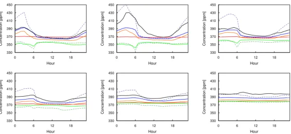
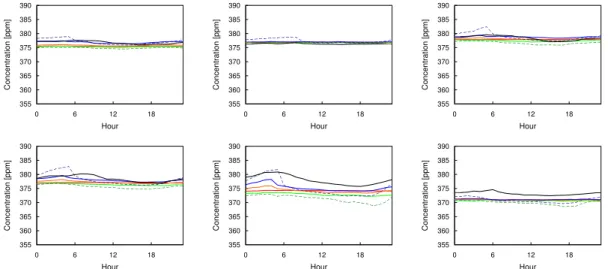
both in terms of correlation as well as in bias. Figure 6shows the monthly averaged

diurnal cycles of the modelled and measured signals. All months have≥75% valid data

coverage except July (16%) and August (59%).

The Mace Head station is used for the purpose of obtaining boundary condition

measurements for the European domain. Figure6shows that the anthropogenic

con-5

tribution is indeed low (red). Larger uptakes of CO2 (dashed and solid green) are

observed during periods with winds from easterly directions when the Irish and UK is-lands and the European continent are within the region of influence. These uptakes are again compensated by autotrophic and heterotrophic respiration (yellow, dashed and solid blue). The night time variability is overestimated when using the SiB3 NEP fluxes

10

(σ₌₁₀._{2 ppm instead of 5.8 ppm). By setting the lower limit for the PBL height to 100 m}

instead of 50 m the performance (R2₌₀._46,σ₌₆._{6 ppm, bias}₌_{–1.4 ppm) improves}

com-pared to Case 6 in Table5(R2₌₀._27,σ₌₁₀._{2 ppm, bias}₌_{–1.8 ppm). However, as was}

the case for the Hegyhatsal site in the previous section, the correlation does not im-prove to the same value as obtained using the FACEM model output. Furthermore, as

15

can be seen in Fig.2, SiB3 tends to predict larger GPP in Ireland than observed by

MODIS, and therefore the heterotrophic respiration fluxes are expected to be relatively

high as well (see Sect.3.1.2. We also expect that the differences can be caused by

the different spatial resolutions of the two biosphere models; The FACEM fluxes are

available at twice the resolution as the SiB3 fluxes. Mace Head is located at 9.54◦W,

20

which is rather close to the border of two adjacent grid-cells and located in the coastal region of Ireland. Falsely attributing terrestrial fluxes to a station with a predominantly marine region of influence can result in over estimation of variability. Indeed, the

per-formance compared to Case 6 in Table5shows further improvement after shifting the

SiB3 fluxes one grid-cell further east (R2₌₀._51,σ₌₅._{3 ppm, bias}₌_{–2.3 ppm). This}

im-25

provement suggests that one can considerably improve the modelled concentrations

for stations that are known to be near to sharp boundaries between different biomes by

(15)

ACPD

8, 4117–4154, 2008

G. Pieterse et al.

Title Page

Tables Figures

◭ ◮

Back Close

Full Screen / Esc

EGU

4 Conclusions

4.1 Flux model evaluation

The FACEM and SiB3 GPP fluxes indicate similar behaviour of both biosphere models

for the central part of Europe, measured by good spatial correlations (R2_≥₀._60),

rea-sonable differences in variability (|∆σ_|≤_{40%) and a small bias (}_≤_{40%) for most regions.}

5

For high latitudes, the availability of accurate LAI data is a limiting factor, especially for the winter season. We expect that implementation of fixed low-values LAI estimates for these region will improve the performance of FACEM for the winter season.

Both models yield significantly different GPP for the Southern part of France. We

suggest that these differences are caused by the different spatial distributions of LAI

10

that are used to calculate GPP; SiB3 and FACEM use the observations of different

satellite platforms to derive this important parameter. For regions with mixed oceanic and continental meteorological conditions, such as Ireland and the United Kingdom, the different spatial resolutions of FACEM and SiB3 (0.₅◦_×₀.₅◦_{and 1}.₀◦_×₁.₀◦_,

respec-tively) di_fferences were also expected and observed; FACEM predicts up to 40% less

15

variability in GPP and 40% lower average productivity than SiB3. Section4.2will

elab-orate more on this subject.

For NEP, similar but more pronounced discrepancies were observed between FACEM and SiB3 model results. Furthermore, FACEM predicts a much larger NEP for

the winter season. This difference can be explained by the fact that the heterotrophic

20

respiration scheme implemented in FACEM does not account for snow cover and frost conditions. It is expected that incorporating such a dependency will result in more representative NEP fluxes for the winter season in the FACEM model.

4.2 Overall model evaluation

The results presented in Sect.3.2show that the combined model framework, i.e. the

25

(16)

re-ACPD

8, 4117–4154, 2008

G. Pieterse et al.

Title Page

Tables Figures

◭ ◮

Back Close

Full Screen / Esc

EGU

producing the measurements of three different sites in the European domain well.

Day-time concentrations were modelled with convincing correlations (R2₌₀.₆₂₋₀._{75). The}

night-time predicted concentrations showed less correlation (R2₌₀.₄₆₋₀._{57). An}

im-portant factor influencing the absolute night time concentrations is the height of the nocturnal PBL. Model results obtained using SiB3 NEP fluxes frequently overestimated

5

night time concentrations for the Hegyhatsal tall tower and the Mace Head station. In the BPL scheme that is implemented in COMET the stable PBL height was limited to a minimum of 50 m. Increasing this lower limit to a value of 100 m and repeating the calculations for SiB3 improved the night-time performance significantly. For

Hegy-hatsal, the performance improved from R2₌₀._44, σ₌₂₃._{1 ppm and bias}₌_{3.5 ppm to}

10

R2₌₀._55,σ₌₁₃._{2 ppm and bias}₌_{–2.2 ppm. For Mace Head, the performance also}

im-proved, fromR2₌₀._27, σ₌₁₀._{2 ppm and bias}₌_{–1.8 ppm to}R2₌₀._46, σ₌₆._{6 ppm and}

bias=–1.4 ppm. However, this did not lead to similar performance as observed when

the FACEM NEP fluxes were used. It is likely that this di_fference can be explained by

the different spatial resolutions of both biosphere models. Especially for sites located

15

near boundaries between oceanic and continental grid cells, such as Mace Head,

us-ing biosphere models with different spatial resolution will lead to significantly different

results. Indeed, the results showed further improvement after shifting the SiB3 NEP

fluxes one grid-cell further east (R2₌₀._51, σ₌₅._{3 ppm, bias}₌_{–2.3 ppm), herewith}

in-creasing the influence of the oceanic fluxes compared to the fluxes of the terrestrial

20

biosphere. The difference in performance could also be explained by the different

ap-proaches followed to calculate NEP. The annual NEP is constrained to zero in SiB3, whereas soil carbon pools are used to calculate heterotrophic respiration in FACEM. For regions with larger modelled GPP fluxes, SiB3 will on average also predict larger heterotrophic respiration fluxes. This can result in over predictions in modelled

night-25

time PBL concentrations when photosynthesis does not contribute.

This work also illustrates the limitations for possible extraction of the biospheric and anthropogenic contributions to atmospheric concentration measurements. The GPP

(17)

ACPD

8, 4117–4154, 2008

G. Pieterse et al.

Title Page

Tables Figures

◭ ◮

Back Close

Full Screen / Esc

EGU

in this study. The sites are typical continuous (tall tower) sites and representative for other sites over the globe. Mace Head is situated in a remote location barely influenced by biospheric and anthropogenic activity. Cabauw is situated in a region with high anthropogenic activity and Hegyhatsal in a region with predominantly biogenic activity.

We therefore expect that it will be di_fficult, if not impossible, to extract the GPP signal

5

directly from atmospheric concentration measurements alone. This problem is mainly caused by well-mixed state of the planetary boundary layer during day time, resulting in significant dilution of GPP information present in the measured signals. Additional flux

measurements could provide better means to separate the signals of the different parts

of the biosphere. Measurements obtained from locations with less pronounced human

10

contributions will allow for a better opportunity to derive the GPP signal. Additional tracers could be very useful to separate the signal due to anthropogenic emissions from

the biospheric fluxes. A possibility is the use of14CO2 measurements (IPCC,2007),

with the disadvantage of the more expensive measurement techniques involved and the low temporal resolution of such measurements. CO measurements do not have

15

this disadvantage, but the CO-to-CO2ratios for the different fossil fuel sources have a

rather wide range (Levin and Kastens,2007) and direct comparison of these two tracers

is therefore limited. Another possibility would be the use of CH4 concentrations as a

proxy for human emissions, but here the disadvantage is that the co-location between

anthropogenic CO₂ and CH₄ sources is far from ideal and that major natural sources

20

of CH4that are not associated with CO2emissions also exist.

The human emissions of CO2 are known quite accurately. A more promising

ap-proach would be to subtract the modelled concentration signals due to anthropogenic emissions from the measured signal followed by a partitioning of the remaining sig-nal between GPP and respiration. During night time, the sigsig-nal is clearly dominated

25

(18)

ACPD

8, 4117–4154, 2008

G. Pieterse et al.

Title Page

Tables Figures

◭ ◮

Back Close

Full Screen / Esc

EGU

available. However, night time conditions are currently still hard to reproduce by at-mospheric transport models and uncertainties introduced by these models will limit accurate footprint analysis for nighttime concentrations. Therefore, quantifying the im-pact of the biosphere on the carbon budget, based on concentration measurements, is expected to remain a tough problem to tackle in the near future.

5

Acknowledgements. We would like to acknowledge the World Data Centre for Greenhouse Gases (WDCGG), the CarboEurope project and Aerocarb project for providing the CO₂ concen-tration measurements required for the model-to-measurement comparisons. Also, we would like to thank T. R ¨ockmann from the Institute for Marine and Atmospheric research in Utrecht (IMAU) in the Netherlands for his valuable comments on this manuscript.

10

References

Aurora, V. K.: Simulating energy and carbon fluxes over winter wheat using coupled land sur-face and terrestrial models, Agr. Forest Meteorol., 118, 21–47, 2003.4122

Baker, I. T., Denning, A. S., Hanan, N. P., Prihodko, L., Uliasz, M., Vidale, P.-L., Davis, K., and Bakwin, P.: Simulated and observed fluxes of sensible and latent heat and CO₂at the 15

WLEF-TV tower using SiB2.5, Glob. Change. Biol., 9, 1262-1277, 2003. 4122

Baker, I. T., Denning, A. S., Hanan, H., Berry, J. A., Collatz, G. J., et al.: The next generation of the simple biosphere model (SiB3): model formulation and preliminary results, in: Proceed-ings of the 1st iLEAPs Science Conference, edited by: Reissell, A. and Aarflot, A., Finish Association for Aerosol Research, Boulder, Colorado, USA, 2006. 4122

20

Baker, I. T., Berry, J. A., Collatz, G. J., Denning, A. S., Hanan, N. P., Philpott, A. W., Prihodko, L., Schaefer, K. M., Stockli, R. S., and Suits, N. S.: Global net ecosystem exchange NEE fluxes of CO₂, Available online [http://www.daac.ornl.gov] from ORNL Distributed Active Archive Center, Oak Ridge, USA, 2007. 4122

Beljaars, A. C. M. and Bosveld, F. C.: Cabauw data for the validation of land surface parame-25

terization schemes, J. Climate, 10(6), 1172–1193, 1997.4126

(19)

ACPD

8, 4117–4154, 2008

G. Pieterse et al.

Title Page

Tables Figures

◭ ◮

Back Close

Full Screen / Esc

EGU Collatz, G. J., Ball, K. T., Grivet, C., and Berry, J. A.: Physiological and environental regulation

of stomatal conductance, photo synthesis and transpiration: A model that includes a laminar boundary layer, Agr. Forest Meteorol., 54, 107–136, 1991. 4121

Denning, A. S., Collatz, G. J., Zhang, C., Randall, D. A., Berry, J. A., Sellers, P. J., Colello, G. D., and Dazlich, D. A.: Simulations of terrestrial carbon metabolism and atmospheric CO₂ in a 5

general circulation model. part 1: Surface carbon fluxes, Tellus, 48B, 521–542, 1996. 4122, 4126

Derwent, R. G., Ryall, D. B., Manning, A. J., Simmonds, P. G., O’Doherty, S., Biraud, S., Ciais, P., M., R., and Jennings, S. G. : Continuous observations of carbon dioxide at mace head, ire-land from 1995 to 1999 and its net european ecosystem exchange, Atmos. Environ., 36(17), 10

2799–2807, 2002. 4127

Globalview-CO₂: Cooperative Atmospheric Data Integration Project – Carbon Dioxide, 2005. 4119,4123

Hazpra, L.: Atmospheric CO₂ hourly concentration data, hegyhatsal (HUN), World Data Centre for Greenhouse Gases, Japan Meteorological Agency, 20 Tokyo, available at: 15

http://gaw.kishou.go.jp/wdcgg.html, 2006. 4127

Heinsch, F. A., Reeves, M., Bowker, C. F., Votava, P., Kang, S., Milesi, C., Zhao, M., Glassy, J., Jolly, W. M., Kimball, J. S., Nemani, R. R., and Running, S. W.: Users guide: GPP and NPP (MOD17A2/A3) products NASA MODIS land algorithm, 2003.4122,4125

IPCC: Climate change 2007: The physical science basis. contribution of working group I to 20

the fourth assessment report of the intergovernmental panel on climate change, in: Fourth IPCC Assessment Report, edited by: Solomon, S., Qin, D., Manning, M., Chen, Z., Marquis, M., Averyt, K., Tignor, M., and Miller, H., Cambridge University Press, Cambridge, United Kingdom and New York, 2007. 4118,4122,4133

Ito, A. and Oikawa, T.: A model analysis of the relationship between climate perturbations and 25

carbon budget anomalies in global terrestrial ecosystems: 1970 to 1997, Clim. Res., 15, 161–183, 2000. 4122

Knorr, W.: Annual and interannual CO₂exchanges of the terrestrial biosphere: process based simulations and uncertainties, Global Ecol. Biogeogr., 9, 225–252, 2000.4122

Knyazikhin, Y., Glassy, J., Privette, J. L., Tian, Y., Lotsch, A., Zhang, Y., Wang, Y., Morisette, 30

(20)

ACPD

8, 4117–4154, 2008

G. Pieterse et al.

Title Page

Tables Figures

◭ ◮

Back Close

Full Screen / Esc

EGU Levin, I. and Kastens, U.: Inferring high-resolution fossil fuel CO₂ records at continental sites

from combined14CO₂and CO observations, Tellus B, 59, 2007. 4133

Olivier, J. G. J., Van Aardenne, J. A., Dentener, F., Ganzeveld, L., and Peters, J. A. H. W.: Recent trends in global greenhouse gas emissions: regional trends and spatial distribution of key sources, in: Non-CO₂Greenhouse Gases (NCGG-4), edited by: van Amstel, A., 325– 5

330, Millpress, Rotterdam, The Netherlands, 2005. 4123

Pieterse, G., Bleeker, A., Vermeulen, A. T., Wu, Y., and Erisman, J. W.: High resolution model-ing of atmosphere-canopy exchange of acidifymodel-ing and eutrophymodel-ing components and carbon dioxide for european forests, Tellus B, 59(3), 412–424, 2007. 4118,4120,4122

Randall, D. A., Wood, R. A., Bony, S., Colman, R., Fichefet, T., Fyfe, J., Kattsov, V., Pitman, 10

A., Shukla, J., Srinivasan, J., Stouffer, R. J., Sumi, A., and Taylor K. E.: Climate models and their evaluation, in: Climate Change 2007: The Physical Science Basis. Contribution of working Group I to the Fourth Assessment Report of the Intergovernmental Panel on Climate Change, edited by: Solomon, S., Qin,D., Manning, M., Chen, Z., Marquis, M., Averyt, K., Tignor, M., and Miller, H., Cambridge University Press, Cambridge, United Kingdom and 15

New York, 2007. 4118

Sellers, P. J., Randall, D. A., Collatz, G. J., Berry, J. A., Field, C. B., Dazlich, D. A., Zhang, C., Collelo, G. D., and Bounoua, L.: A revised land surface parameterization (SiB2) for atmo-spheric GCMs, Part I: Model formulation, J. Clim., 9, 676–705, 1996. 4118,4121,4122 Stohl, A. and Seibert, P.: Accuracy of trajectories as determined from the conservation of 20

meteorological tracers, Q. J. Roy. Meteor. Soc., 124, 1465–1484, 1998. 4123

Stohl, A., Wotawa, G., Seibert, P., and Kromp-Kolb, H.: Interpolation errors in wind fields as a function of spatial and temporal resolution and their impact on different types of kinematic trajectories, J. Appl. Meteorol., 34, 2149–2165, 1995.4123

Takahashi, T., Sutherland, S. C., Sweeney, C., Poisson, A., Metzl, N., Tillbrook, B., Bates, N., 25

Wanninkhof, R., Feely, R. A., Sabine, C., Olafsson, J., and Nojiri, Y.: Global sea-air CO₂ flux based on climatological surface ocean pCO₂, and seasonal biological and temperature effects, Deep-Sea Res. II, 49, 1601–1622, 2002.4123

Teillet, P. M., El Saleous, N., and Hansen, M.: An evaluation of the global 1-Km AVHRR land dataset, Int. J. Remote Sens., 21, 1987-2021, 2000. 4125

30

Ulden, A. P. v. and Wieringa, J.: Atmospheric boundary layer research at Cabauw, Bound.-Lay. Meteorol., 78, 39–69, 1996.4126

(21)

ACPD

8, 4117–4154, 2008

G. Pieterse et al.

Title Page

Tables Figures

◭ ◮

Back Close

Full Screen / Esc

EGU european methane emissions, Environ. Sci. Pollut., 2, 315–324, 1999. 4120,4123

Vermeulen, A. T., Pieterse, G., Hensen, A., van den Bulk, W. C. M., and Erisman, J. W.: Comet: a lagrangian transport model for greenhouse gas emission estimation forward model technique and performance for methane, Atmos. Chem. Phys. Discuss., 6, 8727–8779, 2006, http://www.atmos-chem-phys-discuss.net/6/8727/2006/. 4118,4120,4123

5

Vidale, P. L. and Stoekli, R.: Prognostic canopy air space solutions for land surface exchanges, Theor. Appl. Climatol., 80, 245–257, 2005. 4122

World Meteorological Organisation: WMO WDCGC data summary, volume IV – Greenhouse gases and other atmospheric gases, Japan meteorological agency in cooperation with WMO, 31st edition, 2007. 4119

10

(22)

ACPD

8, 4117–4154, 2008

G. Pieterse et al.

Title Page

Tables Figures

◭ ◮

Back Close

Full Screen / Esc

EGU Table 1.Description of the six cases considered for the model-to-measurement comparison.

Case number Used data set

1 Takahashi

Edgar Fast Track

2 or 5 Takahashi

Edgar Fast Track

FACEM GPP or SiB3 GPP

3 Takahashi

Edgar Fast Track FACEM NPP

4 or 6 Takahashi

Edgar Fast Track

(23)

ACPD

8, 4117–4154, 2008

G. Pieterse et al.

Title Page

Tables Figures

◭ ◮

Back Close

Full Screen / Esc

EGU Table 2. Description of the three European sites considered in the combined COMET and

biospheric model framework.

Site name Longitude [◦] Latitude [◦] Height(s) [m] Description

Cabauw 4.93 51.97 20, 60, 120, 200 Continental

Hegyhatsal 16.65 46.97 10, 48, 82, 115 Deep continental

(24)

ACPD

8, 4117–4154, 2008

G. Pieterse et al.

Title Page

Tables Figures

◭ ◮

Back Close

Full Screen / Esc

EGU Table 3. Model performance for the prediction of CO₂concentrations at the Cabauw tall tower

site, using different data sets for source and sink strength estimates, see Table1.

R2[–] σ[ppm] Bias [ppm]

Measurements – 17.1 –

Measurements (daytime) – 12.9 –

Measurements (nighttime) – 17.6 –

Case 1 0.63 10.0 −7.8

Case 2 0.35 11.4 −12.9

Case 3 0.62 13.7 −7.0

Case 4 0.67 16.7 −1.2

Case 4 (daytime) 0.75 14.0 0.5

Case 4 (nighttime) 0.57 17.2 −2.4

Case 5 0.41 10.6 −14.2

Case 6 0.69 15.1 −3.9

Case 6 (daytime) 0.74 12.0 −2.2

(25)

ACPD

8, 4117–4154, 2008

G. Pieterse et al.

Title Page

Tables Figures

◭ ◮

Back Close

Full Screen / Esc

EGU Table 4. Model performance for the prediction of CO₂ concentrations at the Hegyhatsal Tall

tower site, using different data sets for source and sink strength estimates, see Table1.

Case 1 0.15 4.1 −11.0

Case 2 0.07 10.9 −18.5

Case 3 0.45 8.1 −9.9

Case 4 0.54 9.5 −4.7

Case 4 (daytime) 0.62 8.5 −4.0

Case 4 (nighttime) 0.46 9.2 −5.1

Case 5 0.04 10.8 −20.2

Case 6 0.44 23.1 3.5

Case 6 (daytime) 0.57 9.4 −2.7

(26)

ACPD

8, 4117–4154, 2008

G. Pieterse et al.

Title Page

Tables Figures

◭ ◮

Back Close

Full Screen / Esc

EGU Table 5.Model performance for the prediction of CO₂concentrations at the site at Mace Head,

using different data sets for source and sink strength estimates, see Table1.

Case 1 0.45 4.4 −3.1

Case 2 0.29 5.6 −3.9

Case 3 0.52 5.0 −2.8

Case 4 0.54 6.1 −1.6

Case 4 (daytime) 0.62 5.7 −1.5

Case 4 (nighttime) 0.49 6.4 −1.7

Case 5 0.12 7.4 −4.9

Case 6 0.27 9.1 −0.8

Case 6 (daytime) 0.21 6.9 −1.8

(27)

ACPD

8, 4117–4154, 2008

G. Pieterse et al.

Title Page

Tables Figures

◭ ◮

Back Close

Full Screen / Esc

EGU Fig. 1.The correlation (R2), relative di_fference in the standard deviation (_∆σ) and relative bias

(28)

ACPD

8, 4117–4154, 2008

G. Pieterse et al.

Title Page

Tables Figures

◭ ◮

Back Close

Full Screen / Esc

EGU Fig. 1. Continued. The correlation (R2), relative di_fference in the standard deviation (_∆σ) and

(29)

ACPD

8, 4117–4154, 2008

G. Pieterse et al.

Title Page

Tables Figures

◭ ◮

Back Close

Full Screen / Esc

EGU Fig. 2. Comparison of monthly averaged GPP with MODIS GPP for the Spring (a)–(c)and

(30)

ACPD

8, 4117–4154, 2008

G. Pieterse et al.

Title Page

Tables Figures

◭ ◮

Back Close

Full Screen / Esc

EGU Fig. 2. Continued. Comparison of monthly averaged GPP with MODIS GPP for the Autumn

(31)

ACPD

8, 4117–4154, 2008

G. Pieterse et al.

Title Page

Tables Figures

◭ ◮

Back Close

Full Screen / Esc

EGU Fig. 3.The correlation (R2_{), relative di}_ff_{erence in the standard deviation (}_∆σ_{) and relative bias}

(32)

ACPD

8, 4117–4154, 2008

G. Pieterse et al.

Title Page

Tables Figures

◭ ◮

Back Close

Full Screen / Esc

EGU Fig. 3. Continued. The correlation (R2), relative di_fference in the standard deviation (_∆σ) and

(33)

ACPD

8, 4117–4154, 2008

G. Pieterse et al.

Title Page Abstract Introduction Conclusions References Tables Figures ◭ ◮ ◭ ◮ Back Close

Full Screen / Esc

Printer-friendly Version Interactive Discussion EGU 350 360 370 380 390 400 410 420

0 6 12 18

Hour Concentration [ppm] 350 360 370 380 390 400 410 420

0 6 12 18

Hour

Concentration [ppm]

(34)

ACPD

8, 4117–4154, 2008

G. Pieterse et al.

Full Screen / Esc

0 6 12 18

Hour

Concentration [ppm]

(35)

ACPD

8, 4117–4154, 2008

G. Pieterse et al.

Full Screen / Esc

Printer-friendly Version Interactive Discussion EGU 330 350 370 390 410 430 450

0 6 12 18

Hour Concentration [ppm] 330 350 370 390 410 430 450

0 6 12 18

Hour

Concentration [ppm]

(36)

ACPD

8, 4117–4154, 2008

G. Pieterse et al.

Full Screen / Esc

Printer-friendly Version Interactive Discussion EGU 330 350 370 390 410 430 450

0 6 12 18

Hour

Concentration [ppm]

(37)

ACPD

8, 4117–4154, 2008

G. Pieterse et al.

Full Screen / Esc

0 6 12 18

Hour

Concentration [ppm]

(38)

ACPD

8, 4117–4154, 2008

G. Pieterse et al.

Full Screen / Esc

0 6 12 18

Hour

Concentration [ppm]