Carbon source/sink information provided by column CO<sub>2</sub> measurements from the Orbiting Carbon Observatory

(1)

ACPD

8, 20051–20112, 2008

Carbon flux information from

OCO column CO₂

measurements

D. F. Baker et al.

Title Page

Abstract Introduction

Conclusions References

Tables Figures

◭ ◮

Back Close

Full Screen / Esc

Printer-friendly Version

Interactive Discussion

Atmos. Chem. Phys. Discuss., 8, 20051–20112, 2008 www.atmos-chem-phys-discuss.net/8/20051/2008/ © Author(s) 2008. This work is distributed under the Creative Commons Attribution 3.0 License.

Atmospheric Chemistry and Physics Discussions

This discussion paper is/has been under review for the journalAtmospheric Chemistry and Physics (ACP). Please refer to the corresponding final paper inACPif available.

Carbon source/sink information provided

by column CO

₂

measurements from the

Orbiting Carbon Observatory

D. F. Baker1,*, H. B ¨osch2, S. C. Doney1, and D. S. Schimel3

1

Department of Marine Chemistry and Geochemistry, Woods Hole Oceanographic Institution, Woods Hole, MA 02543-1543, USA

2

Department of Physics, University of Leicester, University Road, Leicester, LE1 7RH, UK

3

National Ecological Observatory Network, Inc., 3223 Arapahoe Ave. Suite 210, Boulder, CO 80303, USA

*

now at: Cooperative Institute for Research in the Atmosphere, Colorado State University, Fort Collins, CO 80523-1375, USA

Received: 21 August 2008 – Accepted: 30 September 2008 – Published: 28 November 2008

Correspondence to: D. F. Baker ([email protected])

(2)

ACPD

8, 20051–20112, 2008

measurements

D. F. Baker et al.

Title Page

Tables Figures

◭ ◮

Back Close

Full Screen / Esc

Abstract

We perform a series of observing system simulation experiments (OSSEs) to quantify how well surface CO2fluxes may be estimated using column-integrated CO2data from

the Orbiting Carbon Observatory (OCO), given the presence of various error sources. We use variational data assimilation to optimize weekly fluxes at 2◦_×5◦ (lat/lon) using

5

simulated data averaged only across the_∼33 s that OCO takes to cross a typical 2◦_×5◦ model grid box. Grid-scale OSSEs of this sort have been carried out before for OCO using simplified assumptions for the measurement error. Here, we more accurately describe the OCO measurements in two ways. First, we use new estimates of the single-sounding retrieval uncertainty and averaging kernel, both computed as a

func-10

tion of surface type, solar zenith angle, aerosol optical depth, and pointing mode (nadir vs. glint). Second, we collapse the information content of all valid retrievals from each grid box crossing into an equivalent multi-sounding measurement uncertainty, factor-ing in both time/space error correlations and data availability due to clouds and thick aerosols (calculated from MODIS data). Finally, we examine the impact of three types

15

of systematic errors: measurement biases due to aerosols, transport errors, and errors caused by assuming incorrect error statistics.

When only random measurement errors are considered, both nadir- and glint-mode data give error reductions of_∼50% over the land for the weekly fluxes, and_∼65% for seasonal fluxes. Systematic errors reduce both the magnitude and extent of these

20

improvements by up to a factor of two, however. Flux improvements over the ocean are significant only when using glint-mode data and are smaller than those over land; when the assimilation is mistuned, slow convergence makes even these improvements difficult to achieve. The OCO data may prove most useful over the tropical land areas, where our current flux knowledge is weak and where the measurements remain fairly

25

(3)

ACPD

8, 20051–20112, 2008

measurements

D. F. Baker et al.

Title Page

Tables Figures

◭ ◮

Back Close

Full Screen / Esc

1 Introduction

By themselves, the well-calibrated, long-term atmospheric CO2 measurements at

Mauna Loa and the South Pole have revealed much of what we know of the func-tioning of the global carbon cycle: the steady rise of global CO₂concentrations driven by anthropogenic fossil fuel burning, the uptake of about half this input by sinks in the

5

oceans and on land, and interannual variability in these sinks that is correlated with El Ni ˜no events and large volcanic eruptions. However, to understand why the carbon cycle responds as it does to the climatic and anthropogenic forcing, and to be able to predict how it will behave in the future, models are needed of the important biogeo-chemical processes in both the oceans and land biosphere. These process models

10

are tuned to agree with data from local study sites, then scaled up to give surface CO2

fluxes globally. When run through atmospheric transport models, these fluxes yield atmospheric CO₂ concentrations that may be compared to CO₂ measurements and used to test and improve the flux models. Atmospheric inverse methods provide a framework for optimizing parameters in the process models or the surface CO2fluxes 15

they produce.

So far, the “top-down” atmospheric inverse approach to validating carbon models has been only marginally successful: where the data are most dense, fluxes may be estimated at continental scales (Baker et al., 2006a), but not at the regional scales needed to provide insight into flaws in the carbon models. Part of the problem is that the

20

transport models have systematic mixing errors, including between hemispheres and out of the planetary boundary layer. The models also have great difficulty representing point measurements, particularly over the continents, using grid boxes 100s of km long on a side. The largest problem, however, is that the spatio-temporal density of the current measurement network is insufficient to correct the surface fluxes at regional

25

(4)

ACPD

8, 20051–20112, 2008

measurements

D. F. Baker et al.

Title Page

Tables Figures

◭ ◮

Back Close

Full Screen / Esc

corrections occurring just in the immediate vicinity of the measurement sites) with a frequency dictated by the cross-continental advection time scale.

Space-based measurements provide the most realistic opportunity to achieve cov-erage at such regional scales. Two satellites specifically designed to measure the column-averaged dry air mole fraction of CO₂ (XCO₂) will be launched soon: NASA’s 5

Orbiting Carbon Observatory (OCO) and the Japanese Greenhouse Gases Observing Satellite (GOSAT). Their instruments measure CO2absorption in the near infra-red (IR)

portion of the reflected solar beam and thus have sensitivity down to the surface, which is required to observe the variable near-surface CO2concentrations most affected by

the fluxes (Olsen and Randerson, 2004). Previous instruments that sensed CO2 emis-10

sion in thermal IR bands had sensitivity mainly in the mid- to upper-troposphere and provided less information about the surface fluxes (Chevallier et al., 2005a, b). Both OCO and GOSAT are in sun-synchronous orbits with early afternoon sun-lit equator crossing times and inclinations of 98◦. OCO’s field of view (FOV), _∼2 km on a side, was chosen that small on purpose, to increase the chances of seeing through holes in

15

the clouds, whose radiative transfer effects decrease the accuracy of theXCO₂ retrieval

algorithm (Crisp et al., 2004). OCO has a maximum cross-track scan width of only ∼10 km; these thin scans are spaced every 25◦in longitude, 99 min apart. In addition to nominal near-nadir pointing, both missions can also point at the sun glint spot; this greatly increases the signal over the oceans, which do not otherwise provide much

20

reflection in the near infrared (Miller et al., 2007). The coverage of the satellite data is still limited, though. Neither mission collects data at night, and they provide very little information on the diurnal cycle of CO₂ since they sample only in the local early afternoon. The 25◦ in longitude separating subsequent OCO passes is large enough to make it difficult to resolve synoptic scale variability; GOSAT scans across track, so

25

(5)

ACPD

8, 20051–20112, 2008

measurements

D. F. Baker et al.

Title Page

Tables Figures

◭ ◮

Back Close

Full Screen / Esc

active sensors (e.g. lidar); more complete spatio-temporal coverage could be achieved by placing scanning sensors aboard a constellation of geosynchronous satellites.

In this study, we quantify how well XCO₂ measurements from OCO will help

esti-mate sources and sinks of CO2 at the surface. We use a tracer transport model to

relate patterns in simulated atmospheric CO₂concentration measurements to the

sur-5

face CO2 fluxes at earlier times that determined them. Due to atmospheric mixing,

measurements at progressively higher layers in the atmospheric column reflect fluxes from increasing broad areas at the surface. The transport model allows this XCO₂

measurement information, weighted properly in the vertical column, to be distributed appropriately to fill in the 25◦ gaps between subsequent OCO passes on any given

10

day. Though OCO cannot clarify the diurnal cycle of flux, it can properly account for variability due to synoptic-scale weather systems when they are modeled well by the transport model. Transport models have often been used in back-trajectory inversions to solve for local fluxes with in situ measurements from aircraft campaigns (Gerbig et al., 2003; Lin et al., 2004). For the more regularly-distributed global flask network, flux

15

inversions based on the “Bayesian synthesis” approach (Enting et al., 1995) have been favored. This method has also been used to determine the information on surface CO₂ fluxes provided by satellite data (Rayner and O’Brien, 2001; Houweling et al., 2004; Miller et al., 2007), although only for monthly fluxes from fairly large emission regions (_∼2000 km on a side) since the number of fluxes solved for was limited by the inversion

20

method. The density of OCO’s data should permit fluxes to be estimated at a finer resolution than this, however.

We solve for the CO₂ fluxes at a 2◦_×5◦ resolution (lat/lon) using a state-of-the-art variational data assimilation scheme (Baker et al., 2006b); optimized time-varying 3-D CO2concentration fields are also produced as a by-product. The fluxes are solved at a 25

(6)

ini-ACPD

8, 20051–20112, 2008

measurements

D. F. Baker et al.

Title Page

Tables Figures

◭ ◮

Back Close

Full Screen / Esc

tial guess of the fluxes. Both Baker et al. (2006b) and Chevallier et al. (2007a) have done preliminary OSSEs for OCO using this approach before. For measurements, they assumed a single measurement per model grid box with a 1 or 2 ppm uncertainty value (1σ), respectively, and with a flat weighting versus pressure in the vertical. Here, we improve upon their assumptions in two ways. First, for each individual retrieval, we

5

use new OCOXCO₂ retrieval uncertainties and averaging kernels (AKs) calculated as

a function of surface type, solar zenith angle, aerosol optical depth (OD), and pointing mode (nadir vs. glint) using the OCO Level 2XCO₂ retrieval scheme forced with

radi-ances simulated by the OCO “full-physics” radiative transfer scheme, taken from B ¨osch et al. (2008). Second, instead of assuming only a single valid retrieval per crossing of

10

each model grid box (takes _∼33 s for our 2◦_×5◦ boxes), we collapse the information content of all valid retrievals across each_∼33 s grid box crossing into an equivalent multi-sounding measurement uncertainty, which is then used in the assimilation. Valid

XCO₂ retrievals are only attempted for cloud-free conditions in which the aerosol OD is

less than 0.30, in order to reduce radiative transfer errors due to scattering. We

com-15

pute the number of valid retrievals for each grid box crossing based on the probability that such cloud-free and low-aerosol conditions exist for each retrieval; these proba-bilities are computed using climatological statistics from MODIS data. We attempt to account for along-track correlations in the XCO₂ measurements when specifying the

equivalent measurement uncertainty for each model grid box crossing. Finally, we

20

(7)

ACPD

8, 20051–20112, 2008

measurements

D. F. Baker et al.

Title Page

Tables Figures

◭ ◮

Back Close

Full Screen / Esc

2 Method

2.1 OCO orbit and resolution choices

The OCO satellite measuresXCO₂, the column-averaged dry air mole fraction of CO2,

in the near-infrared (reflected solar bands) with sensitivity down to the surface, but with a vertical weighting that varies with surface type, aerosol amount, and solar zenith

5

angle (SZA) as described in B ¨osch et al. (2008). It samples a single field of view of up to 2.7 km2every 40 ms over a ground track up to 10 km wide (Crisp et al., 2004). It is in a sun-synchronous orbit taking a single sun-lit pass of data per day at_∼13:30 local time, with_∼25◦in longitude separating subsequent passes. (The local time of the ascending node was just recently changed to 13:30; here we use a 13:18 value specified earlier,

10

but we do not expect this to significantly impact our results.) Examples of the sun-lit portion of the OCO FOV ground track are given in Fig. 1. The OCO ground track repeats precisely after 16 days, a fact that is useful for calibrating the measurements at fixed ground sites. However, as shown in Fig. 1, the ground tracks also achieve a somewhat uniform spatial coverage of_∼3.5◦in longitude after only 7 days. We will use

15

this 7-day period here as the discretization step for our solved-for fluxes, since it gives good coverage over our transport model grid boxes, 5◦wide in longitude. The latitudinal resolution of the model is chosen at 2◦to match that of our meteorological products to give maximum resolution in the predominantly north/south (N/S) direction of the OCO ground tracks. Because the OCO data, occurring once per day locally, cannot shed

20

much insight into the diurnal cycle ofXCO₂, some assumption for the diurnal cycle of

the surface CO₂ fluxes must also be made (see Sect. 2.4 below); this then allows multi-day flux blocks to be estimated in a reasonable way from the data.

2.2 Transport model

An off-line atmospheric transport model (the Parameterized Chemical Transport Model,

25

(8)

con-ACPD

8, 20051–20112, 2008

measurements

D. F. Baker et al.

Title Page

Tables Figures

◭ ◮

Back Close

Full Screen / Esc

centrations. It is driven by pre-calculated meteorological fields (horizontal winds, sur-face pressure, vertical di_ffusion coe_fficient, and cloud-convective mass flux) from the GEOS4-DAS reanalysis (Bloom et al., 2005) for the year 1987, interpolated from the resolution normally input to PCTM (2.0◦_×2.5◦ in lat/lon; 55 vertical layers) to the res-olution of the model version used here (2◦_×5◦ lat/lon; 25 vertical layers). The model

5

uses a vertically-Lagrangian finite volume advection scheme (Lin, 2004) and has sim-ple linear schemes for both dry and convective vertical mixing. The 2◦_×5◦ horizontal resolution used here has the advantage of retaining the full N/S (mostly along-track) resolution of the original winds, while allowing for a relatively long (1 h) step size. Be-cause the measurement information is already explicitly spread 5◦in longitude (mainly

10

across-track) due to the 2◦_×5◦box size, no additional spatial correlations are assumed in this analysis.

The modeled 3-D concentration fields are sampled in as similar a manner to the true OCO XCO₂ measurements as the transport model permits: vertically, using the

averaging kernels computed by B ¨osch et al. (2008), as a function of surface type, SZA,

15

aerosol OD, and nadir or glint viewing mode; horizontally, at the transport model’s 2◦_×5◦ resolution; and temporally, at the model’s integration time step (1 h).

The adjoint of the transport model is needed in the assimilation scheme, to move model-data misfit information backwards in time to compute the cost function gradient direction. The adjoint of the forward model has been computed in an efficient manner

20

by running a linear version of the forward advection scheme backwards, and by com-puting the exact adjoint of the vertical mixing schemes’ column mixing matrices. As shown in Baker et al. (2006b), this adjoint is precise enough to allow the true fluxes to be recovered to within 0.2% after 60 iterations in a perfect model simulation with no measurement errors added.

25

2.3 Data assimilation scheme

We solve for weekly surface CO₂fluxes at 2◦x 5◦in lat/lon, usingXCO₂ measurements

(9)

ACPD

8, 20051–20112, 2008

measurements

D. F. Baker et al.

Title Page

Tables Figures

◭ ◮

Back Close

Full Screen / Esc

data span of 1 year. Both the number of fluxes to be solved for (90_×72_×52=∼35 000) and the number of data values used (365_×1500₌_∼50 000) are at least an order of magnitude larger than that used in typical past time-dependent CO2 inversions (e.g.,

R ¨odenbeck et al., 2003; Peylin et al., 2005b; Patra et al., 2005; Baker et al., 2006a; Rayner et al., 2008). Most of these previous inversions used the “Bayesian

synthe-5

sis method”, a batch least squares technique in which transport basis functions were constructed in separate model runs, either one for each solved-for flux or (backwards in time using the adjoint) one for each measurement, to fill a Jacobian matrix relating fluxes to concentrations. The resulting system of linear equations was solved directly to give both the optimal estimate and the accompanying covariance matrix describing

10

the estimation errors. For problems of the size addressed here, it is not computationally feasible to use this sort of direct method – a more computationally efficient approach is needed.

We have chosen to use a variational data assimilation approach to overcome these hurdles. It is similar to the “4-D Var” methods used in numerical weather

predic-15

tion, except that instead of optimizing an initial condition (the atmospheric state) at the start of a relatively short assimilation window, we optimize time-varying boundary values (surface CO2 fluxes) over a longer measurement span. Baker et al. (2006b)

outline the mathematical details and give some test results using simulated data. R ¨odenbeck (2005) has used a similar approach to estimate monthly CO₂ fluxes from

20

20+years of in situ CO2measurements, and Meirink et al. (2008) have recently used

this method to estimate surface CH4 fluxes on a fine grid from SCIAMACHY data.

Rayner et al. (2005) have used a variational approach for solve directly for parameters in land biosphere carbon models, bypassing the surface fluxes. Over the past sev-eral years, a new class of ensemble filtering methods have also been applied to the

25

(10)

ACPD

8, 20051–20112, 2008

measurements

D. F. Baker et al.

Title Page

Tables Figures

◭ ◮

Back Close

Full Screen / Esc

computational savings as great as the variational methods without needing to use the adjoint to the atmospheric transport model (which is often costly to develop). This may be done, for example, using the ensemble version of a fixed lag Kalman smoother, at the cost of inverting a matrix at each time step whose size is related to the number of parameters estimated across the smoother’s sliding time window. While the ensemble

5

methods hold out great promise for the future, we have chosen to go with the proven computational savings of the variational methods for this study.

The variational method works in an iterative fashion, running an estimate of the sur-face fluxes forward in time through the transport model to derive modeled measure-ments, comparing these to the true measuremeasure-ments, and running these measurement

10

residuals (weighted using assumed measurement error statistics) backwards in time through the adjoint of the transport model to obtain flux corrections, then repeating. The flux inversion is posed mathematically as a minimization problem, with the adjoint run providing the gradient to the measurement portion of the cost function. We use the 2nd-order Broyden-Fletcher-Goldfarb-Shanno (BFGS) method to solve for the flux

15

estimates, obtaining a low-rank covariance matrix for errors in the flux estimate.

2.4 Simulation approach

The assimilation seeks to drive an initial (a priori) guess of the fluxes towards the real-world (“true”) fluxes, using the measurements. In our simulations here, we generate measurements with different error sources added on that attempt to describe the real

20

errors OCO will encounter when it actually flies, then process the measurements with the assimilation method in the same way that we would do with the real data. Since we know the fluxes used in generating the data, we can compare the estimated fluxes to these “true” values to get actual estimation errors. If only random estimation errors are added to the data in a perfect-model setup (see Experiments 1 and 2, Sect. 2.6), the

25

(11)

ACPD

8, 20051–20112, 2008

measurements

D. F. Baker et al.

Title Page

Tables Figures

◭ ◮

Back Close

Full Screen / Esc

statistics over seasons (13 weekly flux values) and over a full year (52 values, as done in Chevallier et al., 2007a).

Our simulation approach has the added benefit of allowing us to quantify the impact of systematic errors, such as measurement biases or errors in the transport model, with the same statistics as for the random error experiments. In the first case, the biases

5

are added when simulating the true measurements; in the second case, different winds are used in the optimization than are used to generate the truth.

For our true fluxes, we use monthly land biospheric fluxes from the LPJ model (Sitch et al., 2003) and monthly ocean fluxes from a biospheric run of the NCAR ocean model (Doney et al., 2004; Najjar et al., 2007); both are then interpolate to daily values.

10

For our a priori fluxes, we use similar fluxes from the CASA land biosphere model (Randerson et al., 1997) and the Takahashi et al. (1999) ocean CO2 flux product.

Figure 2a–c gives snapshots of both sets of fluxes for January and July, as well as their di_fference. While both sets of fluxes show similar features (e.g., the seasonal cycle of net photosynthesis minus respiration in both the northern and tropical land vegetation,

15

uptake of CO2by the extra-tropical oceans versus outgassing by the tropical oceans),

their timing and spatial details vary enough that the prior-truth difference (Fig. 2c) is often as large as the fluxes from either model. Thus, the OCO data hold much promise for improving the models, even if the models appear to be doing a fair job of describing the basic biogeochemical processes at the moment.

20

The prior-truth flux differences (Fig. 2c) show systematic spatial and temporal corre-lations. The spatial correlations are often at fine scales, many times associated with deserts and mountain ranges: thin lines of_±values running parallel to the Canadian Rockies, for example. Because of the physical basis of these differences, we have some hope that the differences between our two sets of models will bear some

re-25

(12)

covari-ACPD

8, 20051–20112, 2008

measurements

D. F. Baker et al.

Title Page

Tables Figures

◭ ◮

Back Close

Full Screen / Esc

ance,P_o, including both correlations and the overall magnitude of the variances, will impact the final assimilated estimate, both the value of the estimate itself as well as how rapidly the assimilation converges to it. We use the absolute value of the actual prior-truth flux difference (Fig. 2d) inP_o for most of our assimilation experiments (see Sect. 2.6), but also use an imprecise estimate (Fig. 2e) in a sensitivity experiment to

5

examine the impact of realistic errors in the assumedP_o.

We have not included fossil fuel fluxes in these simulations: errors in our best es-timate of the fossil fuel source are thought to be small at our 2◦_×5◦ resolution. The net flux uncertainties we obtain over land should thus be thought of as applying to the sum of the fossil and land biospheric fluxes. Similarly, the diurnal cycle of flux is not

10

modeled here, since the OCO data, taken at a single local time per day, cannot resolve it.

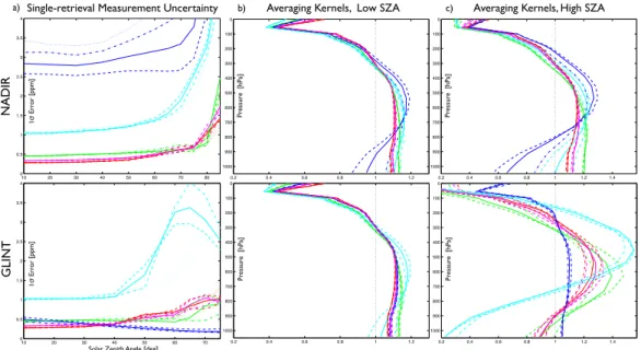
2.5 XCO₂ measurement errors and averaging kernels

The assimilation requires a statistical description of the errors in individualXCO₂

mea-surement retrievals, as well as knowledge of the averaging kernel (AK – how strongly

15

each vertical layer contributes to the column average). Past simulation studies of this sort (Baker et al., 2006b; Chevallier et al., 2007a) have used simplified assumptions for both quantities: flat mass-weighted averages in the vertical, as well as measurement errors of 1 or 2 ppm, with only a single measurement being used in each separate grid box. B ¨osch et al. (2008) have obtained new estimates of both quantities as a

20

function of surface type, SZA, aerosol OD, and pointing mode (nadir vs. glint) (Fig. 3). They used a detailed radiative transfer scheme to simulate the radiances seen in the measured OCO spectral bands, then fed these through the OCO “full-physics” XCO₂

retrieval scheme, testing sensitivities to various error sources. We use these improved error and AK estimates, along with surface FOV locations and SZAs taken from an

ac-25

curate OCO orbit generator for both nadir and glint pointing modes, to calculate realistic values single-soundingXCO₂ retrieval errors and AKs around the orbit.

(13)

ACPD

8, 20051–20112, 2008

measurements

D. F. Baker et al.

Title Page

Tables Figures

◭ ◮

Back Close

Full Screen / Esc

2.7 km2) along the_∼10 km-wide FOV ground track swath crossing any of our 2◦_×5◦ at-mospheric model grid boxes. Since these measurements are taken over an often het-erogeneous surface with di_fferent reflective properties and CO₂emissions, with varying cloud and aerosol amounts interfering with the retrieval, the measurement errors along the swath could be quite variable. When averaged across the grid box, the

uncorre-5

lated portion of these errors could be expected to cancel out significantly. We make an attempt here to estimate what portion of this error cancels out and what does not, to quantify the effective measurement error of all the valid retrievals inside each 2◦_×5◦ model grid box. In computing this e_ffective error, we consider the probability of obtain-ing cloud-free retrievals with aerosol ODs lower than a 0.30 cutoff, and we model

corre-10

lations along the orbit as a function of SZA. The along-orbit computation of the AKs and single- and multi-sounding retrieval uncertainties are done first at a 1◦_×1◦ resolution, then translated to the 2◦_×5◦model grid box resolution based on the time spent in each 1◦_×1◦area inside the 2◦_×5◦box. We show annual mean plots here for the uncertainties and quantities used to compute them, but they vary monthly in the simulations (see the

15

Supplementary Material for seasonal plots http://www.atmos-chem-phys-discuss.net/ 8/20051/2008/acpd-8-20051-2008-supplement.pdf).

Again, we go beyond the previous studies in representing theXCO₂ retrievals in two

ways: 1) we use the more accurate single-soundingXCO₂retrieval errors and averaging

kernels obtained by B ¨osch et al. (2008), and 2) we factor in the combined information

20

available from all retrievals across each 2◦_×5◦ model grid box to compute a lower “ef-fective”XCO₂ retrieval error for use in the flux assimilations.

2.5.1 Single-soundingXCO₂ errors and supporting fields

The calculation of the SZA and the FOV location on the surface, required for theXCO₂

error and AK calculations, both depend on an accurate orbit propagation. For nadir

25

(14)

ACPD

8, 20051–20112, 2008

measurements

D. F. Baker et al.

Title Page

Tables Figures

◭ ◮

Back Close

Full Screen / Esc

angle from the sun and the satellite position vectors, in the plane they define. In both pointing modes, the surface normal is computed assuming the Earth is an oblate spheroid. The orbit is taken as sun synchronous, with a 13:18 local time ascending node, a=7083.45 km, e=0.0012, i=98.2◦. The anomaly is chosen arbitrarily to have the spacecraft crossing north across the equator at 00:00:00 on 1 January.

5

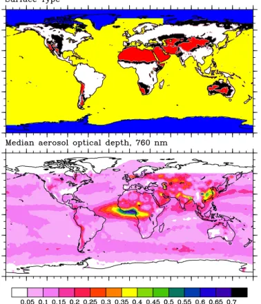
We compute monthly values of SZA and aerosol OD, as well as a constant surface cover type, on the 1◦_×1◦grid. From these, theXCO₂retrieval errors and AKs from B ¨osch

et al. (2008), may be mapped out as a function of position around the globe. These 1◦_×1◦maps are then sampled as a function of position around the OCO orbit to obtain detailed XCO₂ retrieval errors and AKs for use in the assimilation. Figure 4a gives 10

the distribution of the five surface types used to calculate theXCO₂ errors and AKs:

ocean/water, snow/ice, desert, conifer (representing all types of dense vegetation), and sparse vegetation/exposed soil. Figure 4b gives median total aerosol ODs derived from Aqua/MODIS data. The aerosol OD histograms used to compute these medians are described in more detail in B ¨osch et al. (2008). Computed solar zenith angles as

15

a function of latitude for four seasons are given in Fig. 5a. Finally, the OCO single-soundingXCO₂ retrieval uncertainties calculated from these fields are given in Fig. 6a

for both nadir and glint pointing modes. The most striking feature of Fig. 6a is how much lower the uncertainties are over the oceans in glint mode as compared to nadir mode. Note also, however, that they are somewhat lower over the land in nadir mode

20

compared to glint.

2.5.2 Computing effective multi-soundingXCO₂ errors at the 1◦×1◦resolution

Our ability to represent the OCOXCO₂ retrievals is limited by the fairly coarse spatial

resolution of our transport model: a transport model with grid boxes_∼220 km wide can-not represent theXCO₂ variability occurring in the real world at shorter spatial scales. 25

However, for the purposes of estimating CO2 concentrations and fluxes at scales of

100s to 1000s of km, there is no need to model every_∼2.7 km2XCO₂ retrieval correctly.

(15)

ACPD

8, 20051–20112, 2008

measurements

D. F. Baker et al.

Title Page

Tables Figures

◭ ◮

Back Close

Full Screen / Esc

taken inside a model-scale grid box come to the average of all trueXCO₂ values across

the full area of that grid box (not just inside the _∼10 km-wide OCO FOV track)? The model could describe the full-grid-box averageXCO₂ correctly.

The first point to note is that even if theXCO₂ measurements are perfect and

com-plete (no data gaps due to clouds or aerosols) across the full length of the 10 km-wide

5

FOV ground track, there will still be a difference between this perfect ground track average and the averageXCO₂ across the full grid box. Second, the perfectXCO₂

mea-surements may not even get the ground track average correct, because of non-uniform coverage (data gaps) due to clouds and aerosols. And, third, theXCO₂ measurements

are obviously not perfect, but are subject to the measurement errors discussed above.

10

When all the XCO₂ measurements inside a grid box are averaged together, their

er-rors may cancel out to some extent in the average, but there will still be a remaining error between the average measurement and the true XCO₂ value for the measured

portion of the ground track. All three of these errors – track-to-box representation error, along-track representation error, and average effective measurement error – must be

15

combined to get the model-measurement mismatch error that should be fed into the flux error simulations.

The first two of these error sources have been examined by Corbin et al. (2008). They did detailed simulations of XCO₂ variability inside domains of 1◦×1◦ and 4◦×4◦

using a mesoscale atmospheric transport model, comparing theXCO₂ averages along 20

an OCO-like FOV ground track to the average values across the full domain to obtain estimates of the track-to-box representation errors. They also simulated the effect of clouds on the availability of OCO retrievals, coming up with realistic estimates of the along-track representation errors. For the two sites they examined, they concluded that the along-track representation error was small compared to the track-to-box

rep-25

(16)

ACPD

8, 20051–20112, 2008

measurements

D. F. Baker et al.

Title Page

Tables Figures

◭ ◮

Back Close

Full Screen / Esc

the absolute value of the net ocean or land biosphere flux from our monthly-varying a priori flux model inside each 1◦_×1◦ grid box (Fig. 6c, with a proportionality factor of 2.5_×106ppm/kg CO2m−

2

s−1). These track-to-box representation errors are taken to be unbiased and gaussian, and are added in all the simulation cases presented here.

The third error source, the e_ffective joint error of all the individual XCO₂ measure-5

ments inside a grid box, is the largest over almost all of the globe at all times of the year. To compute it, one must factor in data gaps due to cloud coverage or aerosol ODs greater than 0.30 (the level beyond which the OCO retrievals will not be routinely performed). Furthermore, one must estimate the error correlation along the ground track of near-by measurements. Here we assume that errors from aerosols and clouds

10

will dominate the correlated errors (both directly by causing single-sounding retrieval biases that are correlated along-track, and indirectly by introducing data gaps of finite extent that cause representation errors) and that their correlation lengths increase with SZA and path in atmosphere. We represent this with a simple ad hoc correlation length

L:

15

L2=(c2_w+(P _∗c_h_∗tan(SZA))2) (1)

wherecw is a fine-scale cloud width (taken here as 4 km),chis a typical average cloud height (taken here as 7 km), andP is a path-length factor (taken as 1 for nadir pointing mode and 2 for glint). The maximum number of possible independent measurements inside a 1◦x1◦ grid box is then taken to be N_max=p₁◦_×1◦/L, where p1◦_×1◦ is the OCO

20

FOV ground track path length inside the box. This maximum value is reduced by the availability of data due to clouds and aerosols, giving Neff, the effective number of

independentX_CO

2 measurements inside the 1

◦

×1◦grid box, as

Neff =p1◦_×1◦/L∗Pcloud₋free∗(1−PHiAeroOD) (2)

where PHiAeroOD is the probability of aerosol ODs exceeding the 0.30 value beyond 25

which OCOXCO₂ retrievals are not attempted, andPcloud₋freeis the probability of finding

(17)

ACPD

8, 20051–20112, 2008

measurements

D. F. Baker et al.

Title Page

Tables Figures

◭ ◮

Back Close

Full Screen / Esc

is computed from the same aerosol OD histograms as the median aerosol ODs, from B ¨osch et al. (2008). Pcloud₋free is computed from climatologies of Aqua/MODIS and

Terra/MODIS data, sampled in 10 km-wide swaths, as detailed in the Appendix. Both aerosol and cloud coverage are calculated using data from the MODIS instru-ment aboard NASA’s Aqua satellite, which flies in the same “A-train” orbit as OCO will.

5

MODIS has a 1_×1 km FOV that, being close to the_∼2.7 km2 OCO FOV area, should give realistic idea of cloud free areas and aerosol amounts over most areas. Since the MODIS instrument scans up to 45◦off-nadir, the sensed radiation actually passes though a slightly longer path than that for OCO in nadir mode, encountering if any-thing more clouds and aerosols. For OCO in glint mode, however, the path length of

10

the radiation in the atmosphere can be quite a bit longer than that sensed by MODIS. To account for the increased probability of encountering clouds and aerosols at SZAs greater than 20◦ in glint mode, we use these adjusted formulae:

Pcloud−free=P

(2/(1+cos(SZA)/cos(20◦)))

cloud₋free MODIS (3)

PHiAeroOD is recomputed by shifting the 0.30 OD cutoff to a lower value of 0.30* 15

(2/(1+cos(SZA)/cos(20◦))) and summing aerosol OD histogram to the right of this new value. OnceNe_ff is calculated, the effective measurement error accounting for allXCO₂

measurements inside each 1◦_×1◦grid box, is given as: σeff,1_×1=σ1shot/√Neff.

The effective measurement uncertainties at 2◦_×5◦resolution used in the assimilation are then computed from these 1◦_×1◦values, based on the distancel1_×1andl2_×5inside 20

each 1◦×1◦and 2◦×5◦ box, as:l2_×5/σ 2 eff,2_×5=

P

i l1_×1,i /σe2ff,1_×1,i.

Figure 6b gives the distribution ofσeff,1_×1 and Fig. 7, Neff, along with thePcloud₋free

andPHiAeroOD values used to compute them. Figure 7b, c shows that both persistent

cloudiness and areas of high aerosol contamination significantly reduce the availability of OCO measurements in this approach. Theσeff,1_×1values in Fig. 6b are substantially 25

(18)

ACPD

8, 20051–20112, 2008

measurements

D. F. Baker et al.

Title Page

Tables Figures

◭ ◮

Back Close

Full Screen / Esc

these with transport to determine where the flux constraints will be the strongest.

2.6 Flux estimation simulations

The main objective of our study is to perform a series of OSSEs meant to represent how well our data assimilation system will estimate surface CO2fluxes, given the

pres-ence of various error sources. We somewhat arbitrarily divide these errors into purely

5

random ones (modeled as unbiased, gaussian noise) and biases constant in space and time. In reality, of course, there is a spectrum of errors that are correlated in both space and time that fall between these extremes, due to correlations in such error-causing fac-tors as scattering due to aerosols and undetected clouds, spectral e_ffects, and surface reflectance properties. We have attempted to account for some of these terms above

10

by transforming the correlated errors into the corresponding purely random problem using the idea of “e_ffective independent measurements”. Since the finest-resolution unit the atmospheric transport model, and thus the atmospheric flux assimilation, can deal with is the transport model grid box at the model time step, both random and sys-tematic errors are quantified at that scale: what is the net bias or random error between

15

the weighted average of all measurements in a grid box (in a single orbit) and the true concentration in that box?

Table 1 outlines a series of assimilations we perform, with the error sources that have been added in each case. Two of the sources of error described above – the “track-to-box” representation errors and the random measurement errors – have been

20

added in all the experiments as gaussian noise. Biases due the representation errors were found to be small in Corbin et al. (2008) and are not added here at all. Systematic errors in the measurements have been added onto to true measurements in Experi-ments 4–6 (Table 1) described below. Whenever these systematic errors are added, we increase the assumed random measurement uncertainties in an attempt to account

25

(19)

vis-ACPD

8, 20051–20112, 2008

measurements

D. F. Baker et al.

Title Page

Tables Figures

◭ ◮

Back Close

Full Screen / Esc

a-vis the prior and the impact of the biases would be greater than if the measurements had been de-weighted (Chevallier, 2007c). In all experiments, both the measurement error and a priori flux error covariance matrices,RandP_o, are diagonal: we account for correlations in the measurements by computing the effective number of independent measurements and adjusting the multi-sounding measurement uncertainties

accord-5

ingly, and we neglect both time and space correlations between the estimated weekly fluxes at a 1◦_×1◦resolution.

Experiments 1 and 2 can be thought of as “perfect model” experiments for nadir and glint mode data. There is no transport error: the same model that was used to gener-ate the true data is used in the assimilation. There are no measurement biases added,

10

only random measurement errors. And the assimilation is perfectly “tuned”: both the assumed measurement error covariance matrix and the assumed a priori flux estima-tion error covariance matrix are chosen to be consistent with the statistics of the added measurement errors and of the model-truth flux errors, respectively. With these as-sumptions, the flux errors that result from the assimilation should agree with the error

15

statistics that would be given by the a posteriori flux covariance matrix of inverse meth-ods that produce one (our assimilation here does not produce a full rank covariance matrix, only a low-rank approximation not useful for quantitative error analyses at the fine scales examined here). Such a posteriori covariance matrices are often the end product of error analyses and are useful for quantifying the precision of the assimilation

20

(though not necessarily the accuracy, since they do not quantify the impact of system-atic errors). The variances in the a priori flux error covariance matrix were taken to be the square of the actual prior-truth flux difference given in Fig. 2c.

The remainder of the tests were done only for glint viewing mode. In Experiment 3, we add more realism by “mistuning” the assimilation, adding realistic errors to both

25

(20)

ACPD

8, 20051–20112, 2008

measurements

D. F. Baker et al.

Title Page

Tables Figures

◭ ◮

Back Close

Full Screen / Esc

mistune the assumed measurement error covariance matrixR, we actually change the added measurement uncertainties from the glint mode values in Fig. 6b to those shown in Fig. 6d; we keep the assumed values the same as in the other experiments to allow the cost function values to be compared with the other experiments more readily. To obtain the values in Fig. 6d, we simplified the SZA-dependent glint modeXCO₂ retrieval 5

errors (Fig. 3a) as follows: for the conifer and sparse vegetation surface types, the measurement errors were taken to be 0.60 and 0.50 ppm, respectively, for SZAs under 55◦, and 0.70 and 0.90 ppm over 55◦; over deserts and snow, 0.40 and 1.10 ppm under 45◦, and 0.75 and 3.00 ppm over 45◦; and over water, 0.40 ppm for all SZAs.

If only random errors were present in our estimation problem, the results of

Experi-10

ment 3 might give a realistic view of the estimation errors we should expect using the real OCO measurements. Unfortunately, those results will also be corrupted by a range of systematic errors. In Experiment 4, we examine one source of these: measurement biases, taken here as seasonally-varying and proportional to the median aerosol ODs (aero OD) summarized in Fig. 4b. Biases due to aerosols are expected to cause the

15

main systematic errors in the OCOXCO₂ retrievals (Connor et al., 2008). Over land and

ice-covered areas, a bias of+α*aero ODis added to all measurements, while over the ocean, a bias of −α*aero OD is added. The proportionality constant α=1 ppm/OD; the maximum bias is _±0.3 ppm (no XCO₂ retrievals being attempted for aerosol ODs

greater than 0.3). We have also performed Experiment 4b in which twice these aerosol

20

biases were added (α=2 ppm/OD up to a maximum of 0.6 ppm). The magnitude of the biases added in these two experiments range from being comparable to the multi-sounding random measurement uncertainties (1σ) over land in the first case, and twice that in the second case. To account for this extra error in the assimilation, we add the aerosol bias uncertainties given in Fig. 6e to the assumed multi-sounding random

25

(21)

ACPD

8, 20051–20112, 2008

measurements

D. F. Baker et al.

Title Page

Tables Figures

◭ ◮

Back Close

Full Screen / Esc

which scale the biases are added, and 50% of the area under a gaussian curve falls withing_±0.676σ, requiring a larger 1σvalue to represent a bias;√2/0.676₌2.09_≈2)

Measurement errors are not the only systematic errors affecting the flux assimilation: the atmospheric transport models used to relate concentrations to fluxes have a vari-ety of errors, not only in their representation of the broad-scale general circulation, but

5

also in their smaller-scale mixing processes (especially between the planetary bound-ary layer and the free atmosphere). In Experiment 5 we add a version of these instead of the measurement biases. As a simple approximation of these errors, the winds and other mixing parameters that drive the transport model are shifted forward by 17 h in generating the truth as compared to those used in the assimilation. This captures

10

errors in both the synoptic meteorology as well as in the timing of the diurnal cycle of mixing. At the same time, we add the transport uncertainties in Fig. 6f to the as-sumed measurement uncertainties to account for the transport errors; these are taken as the mean of the absolute values of the true and prior fluxes (Fig. 2a, b), divided by the factor 4.0_×10−7kg CO2m−

2

s−1ppm−1between latitudes_±29◦and 2.0_×10−7kg

15

CO2m− 2

s−1ppm−1 outside that. This ad hoc estimate is based on the idea that the largest transport errors occur where the surface flux variability is the greatest, and that this occurs where the fluxes themselves are the greatest. The factor of two difference between the tropics and extra-tropics is meant to account for the greater prevalence of horizontal motions in the extra-tropics that are likely to cause spatial mis-attribution of

20

the fluxes.

Finally, we examine the combined effect of the transport errors from Experiment 5 and the aerosol biases of Experiments 4 and 4b in Experiments 6 and 6b.

3 Results

The goal of our data assimilation approach is to use concentration measurements

25

(22)

ACPD

8, 20051–20112, 2008

measurements

D. F. Baker et al.

Title Page

Tables Figures

◭ ◮

Back Close

Full Screen / Esc

directly estimated by the assimilation, as well as in the seasonal fluxes they imply. (Annual-term mean fluxes would be of more interest for climate research, but since we have only examined a single year we cannot calculate robust error statistics for them; our seasonal mean statistics should be similar to the annual mean ones, we feel.) We make heavy use of the fractional error reduction statistic, given by (RMS_prior–

5

RMSpost)/RMSprior, since it more clearly distinguishes areas of small versus large

im-provement. Finally, we only discuss the RMS errors accumulated across the full annual cycle here; for a seasonal breakdown, see the Supplementary Material http://www. atmos-chem-phys-discuss.net/8/20051/2008/acpd-8-20051-2008-supplement.pdf.

3.1 Perfect-model simulations

10

A posteriori RMS 7-day flux error reductions obtained using data from nadir- and glint-mode OCO observations (Experiments 1 and 2) after several di_fferent de-scent iteration counts of the assimilation algorithm are presented in Fig. 8. (For a direct comparison of the a priori and a posteriori flux errors, see Fig. S4 in the Supplementary Material http://www.atmos-chem-phys-discuss.net/8/20051/2008/

15

acpd-8-20051-2008-supplement.pdf.) The nadir observations provide little improve-ment over the oceans (not surprising, given the very high measureimprove-ment errors there) but impressive improvements over the land – on the order of 45% in most areas, espe-cially where the initial flux errors (Fig. 2c, d) are largest. The glint mode improvement over land is similar in magnitude to that of nadir mode – surprisingly, given that the

20

e_ffective glint mode measurement uncertainties are larger over land than the nadir ones (Fig. 6b). Apparently, enough land flux information blows out over the ocean for the more precise glint mode measurements there to compensate for the less precise and/or less available glint mode measurements over the adjacent land regions. As might be expected, the ocean flux improvement in glint mode is much better than in

25

(23)

ACPD

8, 20051–20112, 2008

measurements

D. F. Baker et al.

Title Page

Tables Figures

◭ ◮

Back Close

Full Screen / Esc

land), we focus on glint mode in the remaining experiments.

Since improvements are less impressive in the areas with low initial flux errors, it appears that the assimilation corrects the largest flux errors during the initial descent steps of the optimization, moving to the finer-scale corrections only later. This flux convergence behavior can be seen in Fig. 9b and 9c, which give the global flux

conver-5

gence in terms of both flux errors weighted as in the cost function (i.e., the error sum that the assimilation seeks to minimize) and the absolute (un-weighted) errors that the eye would see on a flux graph. In terms of both error measures, errors over the land regions are removed first, with the initially-lower errors over the oceans being reduced only later. After iteration 30, in fact, the land flux errors actually grow again in both

10

measures, while the weighted ocean and land₊ocean errors both decrease. Since the lower-flux areas (such as the oceans) were not fully converged after 50 iterations in glint mode, we ran both perfect model cases out to 100 iterations. Figure 8 shows how the ocean errors gradually decrease as the optimization continues, at the cost of higher absolute errors over land. The tradeoffbetween land and ocean errors occurs for both

15

nadir and glint modes in these perfect model simulations.

Figure 9c shows that nadir mode measurements actually give lower absolute (un-weighted) flux errors than glint mode after converging about 25 descent steps – the most converged point on the convergence trajectory for absolute land flux errors as well as absolute land+ocean errors – before the land errors increase again as the

20

assimilation converges smaller absolute flux errors, mostly over the oceans. If we did not care about optimizing fluxes over the ocean, and if we had some way of knowing at which iteration this land minimum was reached in a real assimilation, then we could just stop the assimilation there and achieve the large fractional reductions over land given in Fig. 8c. As Fig. 9c shows, something similar happens with glint mode measurements,

25

(24)

ACPD

8, 20051–20112, 2008

measurements

D. F. Baker et al.

Title Page

Tables Figures

◭ ◮

Back Close

Full Screen / Esc

any improvement over the oceans by setting the a priori flux uncertainties over the ocean to unrealistically low values; the ocean flux values would change little from the a priori values in that case, most of the work done by the assimilation would go towards improving the land fluxes, and there would be only a small rebound in the land errors after the minimum.

5

The a posteriori error statistics given by these perfect model experiments correspond to those from a single draw from the a posteriori estimation error covariance matrix, if our method were to compute one. While they do not include systematic errors, they provide a useful “best case” error estimate – if the measurements are not precise enough to meet their design goals in this view, they never will be when all the other

10

systematic error sources are added in. We address these other errors next.

3.2 Estimation errors with a “mistuned” assimilation

When the measurement noise and a priori flux error covariance matrices assumed in the assimilation (Ra and Po,a) are not equal to those corresponding to the true mea-surement noise added (R_t) and the true statistics of the prior-truth flux fields (P_o,t),

15

then we call the assimilation “mistuned”. For a basic Bayesian cost function

J=(Hx−z)TRa−1(Hx−z)+(x −xo)TPo,a−1(x−xo),

wherex andxorepresent the estimated and a priori state vector,zthe measurements, andHthe measurement matrix, the true a posteriori covariance matrix in that case is given by

20

P_x ₌[HTR−_a1H₊P−_o,a1]−1_[HT_R−1

a RtR−a1H+P−

1

o,aPo,tP−o,a1][HTR−

1

a H+P−

1

o,a]−1 (4)

and no longer reduces to the simplified formPx=[HTR−_a1H+P−_o,a1]−1=P_x,a. To produce a posteriori error statistics corresponding to what would be given by a full-rank covariance matrix with our simulation setup, we had to impose perfect agreement between the assumed errors statistics for the measurement noise and the prior flux errors. We set

25

(25)

ACPD

8, 20051–20112, 2008

measurements

D. F. Baker et al.

Title Page

Tables Figures

◭ ◮

Back Close

Full Screen / Esc

R_a, and we choseP_o,ato agree with the actual (known) prior-truth flux difference. This was done in the perfect model case discussed above (Exps. 1 and 2). However, in a real-world assimilation, one has only an imprecise idea of whatR_tandP_o,t should be, soR_a₆=R_t andP_o.a₆=P_o,t and the covariance from Eq. (4) applies; this is captured in our error statistics when we mistuneP_o,aandR_a.

5

The most noticeable effect of the mistuning of both P_o,aand R_a (Experiment 3), as seen in Fig. 9, is a slowing of the convergence of the descent algorithm. (We have done a separate assimilation, not shown here, that verifies that this slowing is due almost entirely to the mistuning of P_o,a, rather than R_a.) This slowing of the convergence makes sense. The a posteriori fluxes in our assimilation are found using the 2nd order

10

BFGS minimization approach. If one were to know the exact a posteriori covariance matrixP_x at the start, this technique would converge to the optimal estimate in a single step from any prior guess. Of course,P_x is not known beforehand, but a good guess ofP_o, used in setting the starting value of the Hessian matrix, can precondition the search and speed convergence. WhenP_o,a₆=P_o,t, thenP_o,ais a poorer approximation

15

of the prior portion of Eq. (4), P_x,a [P−_o,a1P_o,tP−_o,a1] P_x,a, and thus the minimization is preconditioned worse and takes longer to converge. Put another way, the fine scale spatial detail about the prior-truth difference that one knows ifPo,a=P_o,t is a great help in converging to the truth, but of course would never be known in a real situation.

Because of this slower convergence, we must run the mistuned case (Exp. 3) out

20

many more iterations to get to the same point on the convergence trajectory as in the perfect model case (Exp. 2). After 130 iterations, the 7-day flux results would seem to have convergence to the equivalent of somewhere between iterations 25 and 40 from Experiment 2 (Fig. 8), with perhaps a 10% degradation of the flux improvements (e.g., from 50% to 40%). Probably of greater importance than this error degradation,

25

(26)

re-ACPD

8, 20051–20112, 2008

measurements

D. F. Baker et al.

Title Page

Tables Figures

◭ ◮

Back Close

Full Screen / Esc

mainder of our experiments we will resetPo,a=P_o,t and Ra=R_t and assume that the mistuning errors at a similar point in the convergence trajectory can be added back on after the fact.

For the remaining systematic error experiments, we plot the 7-day and seasonal flux error reductions (Figs. 10 and 11) after 50 descent steps of the assimilation method

5

using glint mode data only. Note that the seasonal mean flux improvements (Fig. 11; RMS of four 13-week spans) are generally similar to the 7-day values (Fig. 10) over the ocean, but significantly higher over the land. For the perfect model case, the initial errors are reduced by over 45% almost everywhere over land, and in many areas where the initial errors were largest, by over 65%.

10

3.3 The impact of aerosol-related measurement biases

Adding a bias proportional to aerosol depth, while compensating for it by increasing the measurement uncertainty (Experiment 4), causes a small degradation in the as-similated 7-day fluxes over land (compare Fig. 10c to 10a; Fig. 9c), most noticeably around the edges of the continents and around the high aerosol regions of equatorial

15

Africa, the Sahara, and India. Over the oceans, the impact is larger, especially in the North Pacific and across the extra-tropical southern oceans. The impact of the biases is more noticeable for the seasonal fluxes (Fig. 11), especially over the land, where most of the flux improvements that were over 75% in the unbiased case are degraded to below that when the aerosol biases are added.

20

When these aerosol biases are doubled (Experiment 4b, Figs. 10d, 11d), the degra-dation is amplified and again the worst effects are over the oceans. The degradation of the seasonal fluxes appears worse than for the 7-day fluxes, perhaps because there is more improvement to lose there. Even so, there are still large areas where improve-ments over 65% remain in the seasonal flux error reductions, particularly in the interior

25

(27)

ACPD

8, 20051–20112, 2008

measurements

D. F. Baker et al.

Title Page

Tables Figures

◭ ◮

Back Close

Full Screen / Esc

3.4 Impact of transport errors

The 17 h shift in winds added in Experiment 5 has the largest impact on the estimated fluxes over the extra-tropics (compare Fig. 10b to 10a), especially over North America and east Asia where the jets are the strongest. The near-surface winds in the extra-tropics are predominantly horizontal, so transport errors there lead to horizontal errors

5

in where the flux corrections are placed. Over the tropics, however, wind motions are more vertical, due to the weak Coriolis force and the dominance of convection; trans-port errors affect more where concentrations are distributed in the column (having little impact on the column-integrated measurement) and less the horizontal assignment of the fluxes. Despite this argument, there also seems to be a sizable degradation in the

10

flux estimates over the tropical Pacific Ocean, perhaps reflecting the importance of the trade winds there.

Compared to the aerosol bias impact, the e_ffect of transport error on the 7-day flux estimates is similar in the tropics, not as bad over the northern oceans, and worse over the extra-tropical continents, especially over North America and parts of Eurasia,

15

leading to larger global flux errors than in either aerosol bias experiment (Fig. 9c). The impact on the seasonal flux error reductions (Fig. 11), however, is different: the trans-port errors generally have a smaller impact than the aerosol bias errors everywhere, except over North America and some ocean areas, where they are similar. Unlike the aerosol biases, which vary slowly across the year, the transport errors are more

vari-20

able and their effect on the inverted fluxes cancels out to a large degree when averaged over longer spans.

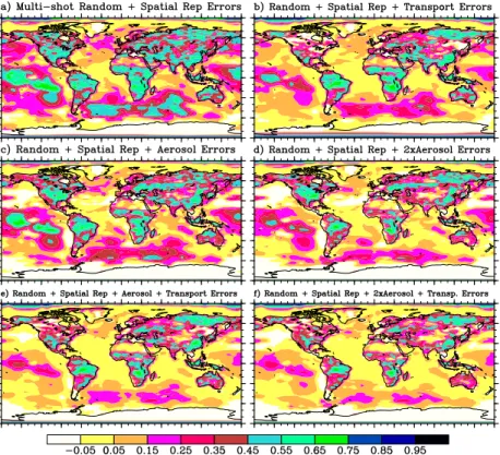
3.5 Impact of both aerosol-related measurement biases and transport errors

When the effects of both transport and measurement bias errors (Exps. 6, 6b) are compared with the effects of either one of the systematic errors (Exps. 4, 4b, and 5) at

25

(28)

ACPD

8, 20051–20112, 2008

measurements

D. F. Baker et al.

Title Page

Tables Figures

◭ ◮

Back Close

Full Screen / Esc

reductions (Fig. 11e, f), there are still broad areas over land with improvements of 50% or higher, even in the doubled aerosol bias case. Error reductions over the oceans are less encouraging, most areas being under 15%. Improvements in the 7-day fluxes are 10–20% lower over the land and similarly low over the ocean. Since the remaining improvement seen in Figs. 10f and 11f were obtained in perfectly-tuned experiments,

5

they must be decreased further by the mistuning effects seen in Fig. 8b to include the effects of all error sources examined here.

There are a few areas where the improvements in Experiment 6 were actually greater than in the individual error source experiments (4 and 5), areas where in Experiments 4 and 5 the assimilation led to results that were actually worse than the prior. This may

re-10

flect mis-tuning of the assumed errors in those experiments: in particular, the additional error added to the assumed measurement uncertainty to account for the transport er-rors (Fig. 6f) may not be large enough or may not have the proper spatial pattern. Erer-rors like this made in incorrectly increasing the measurement uncertainties to account for systematic errors represent another “mistuning” in the assimilation.

15

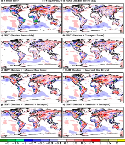
3.6 Impact of systmatic errors at coarser scales

For climate research, flux averages over annual scales (and longer) are of more inter-est than the weekly and seasonal fluxes discussed above. Figure 12 gives the annual mean (a posteriori-true) flux errors for the different error experiments. The correspond-ing fractional error reductions (not shown) are noisy – there is only a scorrespond-ingle term in the

20

required RMS error sums, because only a single year of data was simulated here, so random errors do not cancel out – but, where positive, are generally larger than the seasonal error reductions in Fig. 11. This suggests that the more statistically signifi-cant fractional reductions we obtain for the seasonal flux errors (Fig. 11) may be a good proxy for the annual mean error reductions across the full globe. It was not clear that

25