Optimization of Swirling Flow Energy Parameters on the Velocity Profile after Local Obstacle by Firefly Algorithm

J_{ournal of} A_pplied F_luid M_{echanics, Vol. 10, No. 2, pp. 479-489, 2017.} Available online at www.jafmonline.net, ISSN 1735-3572, EISSN 1735-3645. DOI: 10.18869/acadpub.jafm.73.238.26150

Optimization of Swirling Flow Energy Parameters on the

Velocity Profile after Local Obstacle by Firefly Algorithm

Z. Glav

č

i

ć

1†

, S. Biki

ć

2

and R. R. Bulatovi

ć

1

1 _{Faculty of Mechanical and Civil Engineering in Kraljevo of the University in Kragujevac, Dositejeva 19,}

36000 Kraljevo, Serbia

2 _{Faculty of Technical Scaincs of the University in Novi Sad, Trg Dositeja Obradovia 6, 21000 Novi Sad,}

Serbia

†Corresponding Author Email: glavcic.z@mfkv.kg.ac.rs (Received January 25, 2016; accepted November 10, 2016)

A

BSTRACT

The paper deals with swirling flow (SF) phenomenon which occurs in fluid flow after local obstacle. The phenomenon of SF has been considered in many studies, but here is some different approach to this problem. Based on the theorem of conservation and transfer of energy, a mathematical model of SF was developed in the form of differential equation which defines the velocity profile. During research, special accent was put on the following parameters: swirling parameter, swirling intensity, swirling flux and swirling coefficient. Firefly Algorithm (FA) optimization model, in conjunction with Simulink, was used to get velocity profile vs. time dependence and to verify the developed model. The diagrams of velocity profile were obtained for variation of the initial boundary values of given parameters and conclusions were derived upon mathematical model and simulation of the process.

Keywords: Circumferential component of velocity; Firefly algorithm; Swirling coefficient; Swirling flow; Swirling flux; Swirnling intensity; Swirling parameter.

1.

I

NTRODUCTION

Swirling Flow (SF) phenomenon has occupied minds of researchers for the last few decades and since there occurs circumferential component of velocity which takes away a certain amount of overall flow energy. This effect is very important considering energy aspect of fluid flow. Although there are numerous studies that treat this issue, there is no literature which fully describes all the aspects of SF phenomenon. Because of its complexity and non-stationary nature, SF depends on many parameters and it is almost impossible to take them all into consideration within a single research. Experimental investigation of SF and its mathematical modelling have been present for the last fifty years. One of the earliest investigations in this field was conducted in Benišek (1979), where both the mathematical modelling and the experimental research of SF in a straight circular pipe were done. Recently, researchers conducted simulations of these processes and obtained the results which were used as a platform for further upgrade in this field. Zaets et al. (1998) performed experimental study and mathematical simulation of an axisymmetric turbulent flow in a straight circular pipe and gave a good theoretic base for development of mathematical

models. In addition, the authors investigated distribution and dissipation of turbulence energy

2 0

the relation between the circumferential and axial component was analysed. The diagrams of kinetic energy distribution and energy spectrum were given as well as the diagrams of relation of mentioned velocity components. Research of SF can be related with compressible fluid too, which is presented in Francia et al. (2015). The paper defines axial, circumferential and radial velocity component, which represents the general approach in all papers that deal with SF phenomenon, in both the compressible or in-compressible fluids. Diagrams for each velocity component are given separately for various flow parameters and can be used for comparison purpose and for further development. Particular significance of this paper was in the result obtained via experimental tests, which revealed velocity de-crease and its stabilization after a period of time, also presented in Chang et al. (2014) through kinetic energy. Similar investigations were conducted in some other references, for example in Davailles et al. (2012) and Beaubert et al. (2015), where pressure fields were analysed due to their direct relation with flow velocity profiles. Ubiquity of SF is also shown in Dems et al. (2012), wherein the SF modelling is applied on the large eddy simulation of particle-laden flow. Mathematical modelling was conducted in a similar manner and numerical simulation results revealed similar velocity profiles as in the next referenced papers. In this paper, after setup of the mathematical model, the optimization of SF parameters was carried out in other to validate correctness of this approach.

2.

M

ATHEMATICAL

M

ODEL

One approach in developing the mathematical model that accurately describes the flow process is based on appliance of the general equation of mass, impulse and energy transfer in continuum. Further on, the equations for non-stationary one-dimensional flow are derived from general equations in order to form mathematical models for transient flow processes in hydraulic and pneumatic systems. To develop the mathematical model that describes SF after the local obstacle, it was necessary to start with general law of energy transfer. Although the basic equations are well known, the approach to this issue is some-what different. Therefore, the derivation procedure of mathematical model in terms of the SF basic parameters is presented with some more details. General balance law in the mechanics of a continuum medium is ex-pressed by equations

,

φ ψ

m i j m i j m ki j k

V V A

D

f dV dV dA

Dt



 



 



 (1) where f , ϕ and ψ are arbitrary tensor, vector or scalar fields. The conservation law is formulated if the physical phenomenon is described by general equation of transfer i.e. balance (1).

Parameter Vm is the material volume, i.e. the fluid

volume which consists of the same fluid particles during flow, while D/Dt stands for material derivative.

The right side of Eq. (1) denotes overall influence on considered fluid mass in volume Vm, which leads to

field change of physical value defined by volume integral on the left side of Eq. (1). Values f, ϕ and

ψk denote fields of physical values constrained by formulated physical law, where ϕ and ψ_k are given as functions of value f. In the first integral on the right side of Eq. (1), field can be considered as influence distributed upon overall volumeV_m, while the field ψ_kij denotes influence (e.g. flux), which is applied through material surface Am. This surface is formed by the same fluid particles, so that it continuously encompasses the material volume Vm

in motion.

Starting equation for solving the energy loss problem due to forming the SF is the equation of kinetic energy change in case of one-dimensional non-stationary flow. On the base of energy law, by which the derivative of total energy (sum of internal and kinetic energy) over time for a certain fluid mass equals the sum of power of all forces that act upon it and the exchanged energy per time unit be-tween the fluid mass and surrounding, the general energy transfer law can be written as

2

ρ ρ

2

ρ

m m

m m m

i i

V V

ji i j i i

A V A

D v

e dV F v dV

Dt

p v dA QdV q dA

 

  

 

 

 

  











(2)

where Q denotes the energy production within the volume, and q_i stands for energy flux through the surface in direction of ith coordinate. So, the last two members in Eq. (2) include both the heat ex-change (conduction, radiation, etc.) and the mechanical work exchange (by electric machines and so) with surrounding. In order to obtain the differential form of Eq. (2), it is necessary to per-form the identification of values of f, ϕ and ψ in Eq. (2). Comparing these two equations, the relations follow

2

ρ

2 i j

v f  _e _

 

 , ijρ(F vi iQ) and

ψki_jp vki iqk, by whose further transformations and the use of continuity equation, we obtain the energy equation in differential form

2

ρ ρ( ) ,

2

ji i i i i

j i

p v q

D v

e F v Q

Dt x x

 _ _{  } _

 

  _{ }

  (3)

Kinetic energy change equation is obtained by motion quantity equation multiplying with ,v_i i.e. scalar multiplying of impulse equation by velocity vector

2

2 2

ρ ρ ρ ρ .

2

+ . . ji

i i i j v

D

p D v

F v v F v

Dt x Dt

v DivP

   

  _{  }

 _{      }

 

 _{ }  



Internal energy change equation is now easily obtained by subtracting the kinetic energy Eq. (3) from total energy Eq. (3). It is obvious that a part of surface forces power, given by expression

i ji j v v p x     

is spent on fluid internal energy change. The fluid kinetic energy is changed by the power of surface forces, determined by expression

. _i ji . x y z .

j

p p p p

v DivP v v

x x y z

       _   _  _    _     

To apply the mechanical energy change law to a certain system, i.e. a certain fluid mass, it is necessary to write Eq. (4) in an integral form. To achieve we use this relations

, ,

1 2

ji i ji i

i ji

j j j

j j

i i

ji ji ji ji ji

j i i j

p v p v

v p

x x x

v v

v v

p p p p s

x x x x

 _ _          _  _   _  _ 

(5)

based on stress tensorp_jisymmetry and definition of deformation velocity tensor. Based on Eq. (4), the low of kinetic energy increase, written for a certain fluid mass in material volume Vm, reads as follows

2

ρ ρ

2

.

m m m

m

i i ji i j

V V A

ji ji V

D v

dV F v dV p v dA

Dt

p s dV

 













(6)

This expression, considering later appliance, in some cases can be formulated in more convenient form. For example, if the field of volume forces Fi has its potential U x t( , )_i then by relations

, ,

i i i i

i i

U U DU U

F F v v

x x Dt t

  

      

   (7)

Eq. (4) gets the form 2

ρ ( ) ρ

2

ji i

j p

D v U

U v

Dt t x

 

  

  (8)

whence combined with Eqs. (5) and (6) we obtain the integral formulation of law on kinetic and potential energy increase of a certain material system, i.e. considered fluid mass. The Eqs. (7) and (8) are well known in fluid mechanics literature, but it is important to mention them in order to clearly notice the connection with obtained mathematical model in this paper. When this integral form of mechanical energy law is written for the control volume V on the base of relations (6) and (8), we get

2 2

ρ( ) ρ( )

2 2

ρ .

i i

V A

ji i j ji ji

V A V

d v v

U dV U v dA

dt U

dV p v dA p s dV

t          











 (9)

Tensor field of total stress for Newton fluid is determined by generalized Newton hypothesis,

which defines the linear relation between the stress tensor p_ij and deformation velocity tensor s_ij, where τ_ijstands for viscous stress tensor. When τ_n denotes the stress vector due to viscosity, while T denotes viscosity stress tensor, we can write

τ τ ,

τ . ,τ τ τ τ τ .

ij ij ij n n

n n x x y y z z i i

p p P pE T p pn

T n n n n n

                           (10) When the expression for p_ijand s_ij,relation for are inserted in case of incompressible fluid (v_k/x_k) into the Eq. (6), while using the relation (1), it is obtained

2 2

2 2

ρ

i i i i

V A V

j i

i i i j

A A V

j i

d v v

dV v dA F v dV

dt

v v p

v dA v v dA dV

x x          _  _      













(11)

where the dissipation function  τ_{ij ij}s for incompressible fluid is determined by

2 2 2

1 1

τ τ 2η η( ) .

2η ij ij 2

j i ji ji j i v v s s x x          

 

(12)

Equations (9) and (11), along with relations (7) and (8) give the Bernoulli equation for non-stationary flow

2 2

ρ ρ . ρ .

2 2

( . ). ρF τ .

V A A

i ij

A V V

j

v v

dV v ndA v ndA

t

v

T n vdA dV dV

x  _{   }      













    

  (13)

By separation of surface and volume integrals out of Eq. (13), we obtain the Bernoulli equation for non-stationary SF of viscous incompressible fluid for the finite volume in the form

2

2

(ρ ρ ) . τ . 2

ρ ( ) 0

2

n A

V v

p U v n v dA

V dV t              _    _       





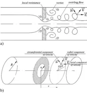
    (14)

Main difference in flow condition before and after the local obstacle is in distribution of velocity and pressure field. Namely, before the local obstacle, the velocity field consists of axial velocity component only, while after the obstacle we also have velocity components in circumferential and radial directions. Total flow velocity square is

2 2 2 2

φ x r

v v v v (15) where:

x

V − axial component of flow velocity along axis x,

r

V − radial component of flow velocity, φ

Therefore, swirl generation after the local obstacle in case of non-stationary flow is characterized by occurrence of circumferential velocity component

φ V .

Based on numerous researches, it is important to notice that the radial velocity values are considerably lower compared with axial and circumferential component. They can be neglected, i.e. v_r0. This fact is very important, because we can conclude, based on the continuity equation, that axial velocity component is the function only of coordinate r and time t, i.e. v_xv r t_x( , )So, at SF formation after the local obstacle, the velocity field can

a)

b)

Fig. 1. Scheme of SF and velocity components after local obstacle.

be defined by the relation v2v2_xv_φ2 . By previously defining the velocity field, the SF parameters are defined. Namely, through averaged circulation

2 2 0

4 R

x r v v dr

V 



 

_



defined are:

Swirling parameter, i.e. the parameter of swirling flow

0 0

, R

x R

f x v rdr V

R _{R rv v rdr}

  









 (16)

Swirling intensity, which represents the relation of fluxes of circumferential flow kinetic energy and axial flow kinetic energy

φ φ

2 2

0

3 ₃

0 ,

x

R

x x

A

R x A

v v dA v v rdr

v dA _{v rdr}

 









_

(17)

Swirling flux, which represents the relation of the

motion quantities momentums in circumferential and axial direction

2

φ ₀

2 ₂

0

R f x x

A

R

x _x

A

r v v dr rv v dA

S

v dA _{rv dr}











_

(18)

So, the main difference between the swirling and non-SF after the local obstacle is the occurrence of circumferential component of flow velocity. Hence, the proper choice of mentioned velocity component profile is a very significant task at modelling the swirling flow. Researches show that near the pipe axis this velocity is proportional to the coordinate r, while near the pipe wall, it is inversely proportional to it. Thereby, we constantly should keep in mind that circumferential component of flow velocity occurs as result of flow nonstationarity, so it must de-pend on time. Besides, the circumferential velocity component can be expressed as a part of axial flow velocity. After each member of Eq. (14) analysis, the mathematical model of SF after local obstacle in hydraulic/pneumatic system can be formed. Including all modelled members into Eq. (14) we obtain the mathematical model of SF as

2 2

2 1

2 1 2 1 2 1

2 2

ρ(α α ) ( ) ρ( )

2 2

1 ρ

ρ λ 0.

2 2

v v

v

v v

x x

u u

p p U U

du u

u dx dx

x dt

     



   







(19)

The last Eq. (19) represents the original equation that came of general flow laws appliance, which are given through Eqs. (1-18), that in various forms al-ready exist in the known literature. Equation (19) is the starting equation on the base of which we would later on come to differential equation of swirling flow. During the model derivation we start from the form that is convenient for simulation which further enables the obtaining the diagram and the analysis of influential parameters on the velocity field after the obstacle.

Variables in Eq. (19) are the field of averaged axial velocity component, i.e. current average velocity u and its derivative over time du/dt. But, except them, there also occur current values of velocities, i.e. u₁ and u₂ , which creates difficulties in forming the differential equation that would depend on velocity and its first derivative over time. So, we rather use the equations that define the overall (to-tal) flow energy. By them, Eq. (19) is written as follows

2 2

2

1 ρ

ρ ρ λ 0

2 2

v

v _{x x} v v

u du u

u dx dx

h t dt

     







0.34 0

0.012

α

α α+A ,

x

v e R



 

 (21)

where: A_α − swirling coefficient, α − Coriolis coefficient of axial non-swirling flow, ₀− swirling parameter at the local obstacle, x− the distance from local obstacle cross section and R− pipeline radius. So, for further analysis of Eq. (20), it is necessary to represent the Boussinesq coefficient of SF in function of already introduced integral parameters. The literature already gives the dependence be-tween Coriolis and Boussinesq coefficient, which reads

α3 2. (22)

For swirling flow, when influences of axial and circumferential flow components are separated, it reads φ φ 3 2 3 2 2 2 1

α ( ),

1

( ).

v _A x _A x

v _A x _A

v dA v v dA Au

v dA v dA Au    









(23)

Transforming the Eq. (19), it can be written

φ φ 2 3 3 3 2 2 2 2 1

α (1 ) ,

1

(1 ) .

x A

v _A x

x A

A

v _A x

x A

v v dA v dA

Au v dA

v dA v dA

Au v dA

     _  _            





_





_

(24)

From all the above, the expressions (24) are transformed into

α_vα(1+ ) (25)

φ

2 2 (1+ A ) v x A v dA v dA 





(26)

From expression (26), we can define the coefficient

φ 2 2 A v x A v dA E v dA 





(27)

that can be named as energy parameter of swirling flow, because it presents the ratio between the kinetic energies of circumferential and axial flows. The higher the value of this parameter the higher the value of circumferential component of SF velocity, i.e. the swirling is more in-tense. From expressions (18) and (19) it follows

(1+ )

v Ev (28) Algebraic transformations lead to the dependence

1 2S

  (29)

out of which we can conclude

1 2 S



 (30)

So, the Boussinesq coefficient of non-swirling axial flow depends on integral parameters of swirling flow. Now it is possible to find the dependence

(α ).

v f v Based on the expression (28) it follows that Boussinesq coefficient of swirling flow, expressed via SF parameters, gets the form

1+ 2 v v E S 

 (31)

Parameter expressed by eq. (31) is energy parameter, very important for the analysis from the point of flow energy efficiency, because it depends on the energy parameter that directly reflects the swirling intensity. By algebraic transformations, swirling flux S and swirling parameter Ω are included through relation

3 1 8 S

  (32)

In eq. (20), its only left to define the friction co-efficient of SF . Some papers, applying the least _v squares method, show that experimental results can be shown by analytic relation

0,42 0,048 0 0,007 1,985 0 λ 1,82 1

λ _{( )}

v

S e    



(33)

where: λ−friction coefficient of axial, non-swirling flow,  ₀ SFparameter immediately after local obstacle, so in the income cross-section. In this way, all elements of eq. (20) are shown through the SF parameters and the mathematical model of the mentioned flow can be established. Based on experimental results, it can be established the following dependence 0,34 0 0,012 α α α x R

v A e

 

  (34)

where: A_α swirling coefficient, α−Coriolis coefficient of axial non-swirling flow. Levelling the expression (25) where and the expression (34), we get the following dependence

0,34 0 0,012 . α α x R A

e 



 (35)

on the base of which eq. (22) reads α 2 3



 .

Inserting eq. (35) in the last relation, we finally obtain

the dependence of Boussinesq coefficient for SF as

0,34 0 0,012 . α ₂ (1 ) 3 x R v v A e E    

  (36)

that is 0,34 0 0,012 . α 2 (1 ) 3 x R v v A e E      

The mathematical model given by Eq. (20) can be transformed in the form

2

(ξ ρ_v + v ρλ_v) 2ρ _v 0

x x

du

dx u dx

t dt

 _{  }







(38)

Inserting Eq. (37) into Eq. (38), with previously solved integral, we get the following equation

0,42 0,048 0

0,34 0

2 0,14

1,985 0

0,34

0,012 .

α 0

1,82λ

ρ(ξ λ )

1 0,024ρ

( 2 ) 0.

3

v

S

x

v R R

u e

E lA du

e l

dt

 

 

 

  





   



(39) Equation (39) can be written as

2

. 0

du C u

dt  (40) Where

0,42 0,048 0

0,34 0

0,14 1,985 0

0,34

0,012 .

α

0 1,82λ

ρ(ξ λ ) /

1 0,024ρ

/ ( 2 )

3 v

S

x

v R R

C

e

E lA

e l

 

 

 

 

 

_   _

 _ 

 

 _ 

 _{ } 

  

 

(41) Equation (39), i.e. Eq. (40), represent the differential equation that mathematically describes the SF after local obstacle. Naturally, it should be stressed that model (39) is just one of possible models. It is given in function of swirling parameters and out of it we can obtain the velocity field in function of already mentioned parameters. This paper presents a special manner of model development. In this model, one should consider four parameters that influence the distribution of velocity field: Aα−swirling co-efficient, Ω0−swirling parameter, T heta−swirling intensity and S−swirling flux. Research and combining of these parameters values lead to velocity profile and conclusions that are a base for further research. It should be mentioned that the velocity u represents velocity field observed from the local obstacle down the flow. As the flow velocity it-self could take different values, a non-dimensional velocity is used in the model and the simulation. It takes value 1 at the local obstacle because the ratio of maximum and current values is u_max/u1. Down the flow, the velocity value, according to the continuity equation, decreases, so the non dimensional velocities take values less than 1.

3. O

PTIMIZATION

O

F

S

F

E

NERGY

P

A

-R

AMETERS

3.1 Short Description of Firefly Algorithm

(FA)

Firefly Algorithm FA first was introduced by X.S. Yang (2009). For forming FA it is necessary idealize some characteristics of firefly flashing light. Here, there are used three idealized rules Yang (2014):

-All reies are unisex so that one rey will be attracted to other reies regardless of their sex;

-Attractiveness is proportional to their brightness, thus for any two ashing reies, the less brighter one will move towards the brighter one. The attractive-ness is proportional to the brightattractive-ness and they both decrease as their distance increases. If there is no brighter one than a particular rey, it will move randomly;

-The brightness of a rey is affected or determined by the landscape of the objective function. For a maximization problem, the brightness can simply be proportional to the value of the objective function.

Based on these three rules, the basic steps of the rey algorithm (FA) can be summarized as the pseudo code shown in Algorithm 1.

Algorithm 1. Firefly algorithm FA (Yang (2009)) 1: begin

2: Objective function f x x( ), ( , x x_{1 2},...x_d)T

3: Define the total fireflies number in population n 4: Generate initial population of fireflies

=(1,..., ) i

x i n

5: Define the number of variables d

6: Light intensity I_i and x_iis determined by ( )f x_i 7: Define light absorption coeficient

8: while (k < MaxGeneration) 9: for i = 1: n %% all n fireflies 10: for j= 1: i%% all n fireflies 11: if (I_jI_i)

12: Move firefly i towards j in d dimension

13: Attractiveness varies with distance r via exp

[-γr]

14: Evaluate new solutions and update light intensity

15: end if 16: end for j 17: end for i

18: Rank the fireflies and find the current best 19: end while

20: Postprocess results and visualization 21: end

In FA algorithms, of special significance are: light intensity variation and attractiveness formulation. For simplicity sake, it always can be assumed that attractiveness of a single firefly is determined by intensity of light flashing, which is related to the value of objective function (Yang 2009, Yang 2014, Arora and Singh 2013).

problems, the brightness I of a rey at a certain location x can be chosen as I (x) ∝ f (x). However, the attractiveness is relative, it depends on beholders impression or on the other reies judgements. So, it will vary with the distance ri j between rey i and rey j. Additionally, light intensity decreases with the distance increase from its source. The light is also absorbed, so the attractiveness should be allowed to vary with the degree of absorption. In the simplest form, the flashing light intensity I(r) varies according to the inverse square law I r( )I_s/r2 where I is the intensity at the source. For the given medium with a fixed light absorption coefficient , the flashing light intensity varies with the distance r

0

( ) r

I r I e (41) where I₀is the initial flashing light intensity. To avoid the singularity at r = 0 in the expression

2

/

s

I r , the combined effect of both the inverse square law and absorption can be approximated by the equation

2

0 ( ) r .

I r I e (42) The firefly’s attractiveness is proportional to the light intensity, thus we can define the attractiveness of a firefly by

2

0

0 ₂

( )= or 1 r

r e

r

 _

 (43)

where ₀is the attractiveness at r = 0. The distance between any two fireflies i and j at x_i and x_j, respectively, is the Cartesian distance

2

, ,

1

( )

d

ij i j i k j k

k

r x x x x



  



 (44)

where x_{i k,} is the kth component of the spatial coordinatex_iofithfirefly. In 2 − D case, we have

2 2

( ) ( ) .

ij i j i j

r  x x  y y

The movement of a firefly i attracted to another more attractive (brighter) firefly j is defined by

2

0

1

( ) α( )

2

ij

r

i i i j

x  x e x x  rand (45)

where the second member stands for the attractiveness influence, while the third member is randomization with being the randomization parameter rand is a random number generator uniformly distributed in [0,1].

The characteristic length is defined as  1 / , through whose value the attractiveness drastically varies from ₀ to ₀e1, i.e. ₀/ 2.

The parameter characterizes the variation of the attractiveness, and its middle value is very important in determining the speed of the convergence and deter-mines how the FA algorithm behaves. In theory,  [0, ] but in practice, = (1)O is determined by the characteristic length Γ of the system to be optimized. Thus, in most applications, it varies from 0.01 to 10.

3.2 Objective Function

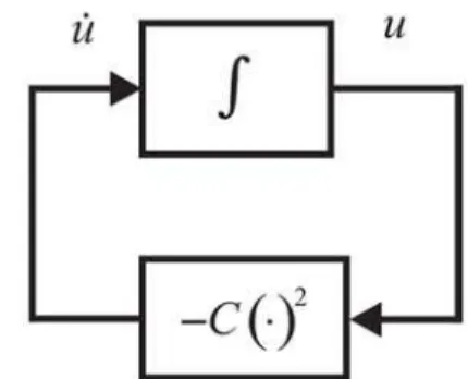
Optimization process is related to solving the Eq. (40). For this, Simulink was used and its block diagram is shown in Fig. 2.

Fig. 2. Model equation block diagram.

Coefficient C, existing in Eq. (40), depends on parameters which are being optimized: A_α,₀, 

and S. FA algorithm calculates the values of these parameters, which are within the given boundaries. Based on the parameters’ values, determined by FA, the new value of coefficient C is calculated, and then this value is sent to Simulink model. Also, the function initial value u(0) is sent to Simulink. Running the Simulink model, two vectors are obtained: u that contains function values for particular time values in vector t. As the objective function, sum of squares of vector u elements is adopted:

2 1

N

obj i

i

F u

 



where N denotes the dimension of vector u. The lower the sum, the lower the surface under function

( ).

u t When FA is finished, the function u t( ),

obtained for optimum values of parameters, is shown.

4. R

ESULTS

In all optimization cases, the algorithm parameters are: n = 20− number of fireflies, α = 0.25, = 0.9, 0 = 0.9, maxiter = 50− maximum number of iterations and d = 4− number of variables being optimized.

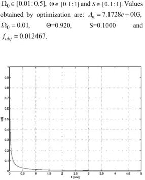
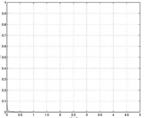
First case

0 [0.01: 0.5],

   [0.1 :1]andS[0.1 :1].Values obtained by optimization are: A_α7.1728e003,

0 0.01,

  Θ=0.920, S=0.1000 and

0.012467. obj

f 

Fig. 3. Velocity dependence on time in the first case.

Second case

Range of project variables is: A_α[1:1000],

0 [0.01: 0.5],

  Θ∈ [0.1 : 1] and § ∈ [0.1 : 1].

Values obtained by optimization are: α 219.2044

A   ₀ 0.102,Θ = 0.8512, S= 0.1948 and fobj0.000215.

In the first phase of parameters optimization, the influence of swirling coefficient A_α and swirling parameter at the point of local resistance ₀on the transient process time was investigated. To get the clearer image of these parameters, their boundaries were changed for the initial values in presented optimization cases. The optimization of parameter Aα is firstly conducted in the range A_α[1:1000]

and then in the range A_α[1000 :10000],in order to encompass the widest possible interval of values of this coefficient. In Figs. 3 and 4, we can notice various times of transition process calming. The calming time also directly depends on the swirling parameter value at the local resistance ₀.So, it was optimized, too, in two ranges also: firstly for

0 [0.01: 0.5]

  and then for  ₀ [0.5 :1]which is depicted in Figs. 5 and 6.

The parameter’s optimum values, A_α219.2044

and thanA_α155.5,were determined. The result of this difference is the increase of transition process time. Namely, as Figs. 3, 4, 5 and 6 show, for optimum values A_α219.2044 and  ₀ 0.102,

the calming time is about 0.1s, while in case when Aα = 155.5 and  ₀ 0.5, the calming time is approximately 5s.

Since the swirling parameter is directly related to the fluid flow, i.e. to the velocity field, characterized by existence of axial and circumferential velocity component, it can be concluded that the higher value of this parameter corresponds to longer calming time.

As the diagrams confirm this fact, we can conclude that the model reflects the process physicality. Naturally, the values of mentioned parameter depend on the values of parameter Aα itself, but also on the values of other SF parameters.

On the other hand, Fig. 4 and 6 indicate the fact that when the values of SF coefficient are in the range A_α[1000 :10000], and the range

0 [0.01: 0.5]

  changes, and then  ₀ [0.5 :1], then the calming time for Aα = 7172.8 is higher than when A_α8614.5 . This relation of parameters is a result of expression (21) dependence from which

0,34 0

0,012 .

α _0,34 α

0

α α

or (α α) 0,012 .

x

v R

v

A A e

x R

 

  



from which we can see that it depends on Coriolis coefficient difference between swirling and non-swirling flow. The higher the difference, i.e. the higher the coefficient A_α value, the higher the energy loss, thus the lower the flow velocity value. Surely, this value depends also on swirl parameter

0,

 which diagrams confirm. Equally, higher value of parameter ₀ responds to higher value of coefficient A_α8614.5,which the last dependence shows.

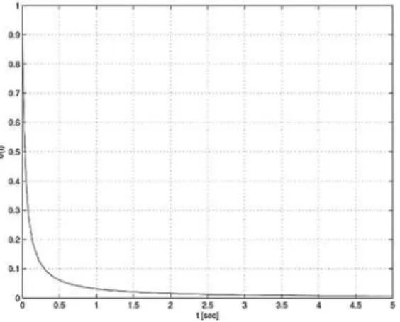
Fig. 4. Velocity dependence on time in the second case.

Third case

Range of project variables is: A_α[1:1000],

0 [0.5 :1],

Fig. 5. Velocity dependence on time in the third case.

Values obtained by optimization are:A_α155.5316

0 0.500,

   1.000, S0.6222 and

0.575412. obj

f 

Fourth case

Range of project variables is: A_α[1000 :10000],

0 [0.5 :1],

   [0.1 :1]andS[0.1 :1].

Values obtained by optimization are: α 8.6145 003,

A  e  0 0.500, Θ = 1.000, S =

0.5622 and f_obj 0.085555

Fig. 6. Velocity dependence on time in the fourth case.

Fifth case

Range of project variables is: A_α[1:1000],

0 [0.01:1],

   [0.1 :1] and S[0.1 :1]. Values obtained by optimization are: A_α.

0

2.8689 003, 0.0100, 1.000, 3.5636 and _obj 0.000164.

e S

f

     

 ..

Second set of parameters optimization is directed to the optimization of swirling intensity Θ and swirling flux S. Namely, this optimization set investigates the influence of ratio between kinetic energies of circumferential and axial flow velocities, i.e.

investigates the influence of motion quantities of these two velocity components.

Fig. 7. Velocity dependence on time in the fifth case.

For this investigation set it is A_α[1:10000] and 0 [0.01:1]

  in order to investigate the influence of two remaining parameters. In Figs. 7 and 8 the swirling flux influence was researched and presented, due to its interval change from S ∈ [0.1 : 1] to S ∈ [1 : 10]. The observed parameter contains first power of circumferential component of velocity in relation to the axial component value, so that there is expected its lower influence on the process calming time in comparison to previous swirling parameter. It is exactly what the diagrams 7 and 8 present, because here the calming time for optimum values S = 0.4271 and S = 0.228 varies from about 3s to 0.5s, respectively. Calming time variation is slightly lower than in case of optimization of swirling parameter and swirling coefficient, which should have been expected and additionally con-firms the model validity regarding the process nature.

Sixth case

Range of project variables is: A_α[1:10000],₀∈ [0.01 : 1], Θ∈ [0.1 : 1] and S ∈ [1 : 10].

Values obtained by optimization are: A_α  0

2.93988 003, 0.0406, 0.2282, 2.2668 and _obj 0.078542.

e S

f

     



Seventh case

Range of project variables is: A_α[1:10000],₀∈ [0.01 : 1], Θ∈ [1 : 10] and S ∈ [1 : 10].

Values obtained by optimization are: A_α  0

2.8689 003, 0.0100, 1.000, 3.6536 and _obj 0.000164.

e S

f

     



figures only in one place, and it is not a part of the function where parameters ₀ and S exist.

Fig. 8. Velocity dependence on time in the sixth case

Fig. 9. Velocity dependence on time in the seventh case.

Fig. 10. Velocity dependence on time in the eighth case.

Eight case

Range of project variables is: A_α[1:10000],₀∈

[0.01 : 1], Θ∈ [1 : 10] and S ∈ [0.1 : 1].

Values obtained by optimization are: A_α 0

3.8991 003, 0.0237, 7.8912, 1.000 and _obj 0.000204.

e S

f

     



This is just a part of the research and there is a great number of possibilities to obtain other dependences and diagrams.

5. C

ONCLUSION

The paper presents the original mathematical procedure which led to formulation of physics-mathematical model of swirling flow, which occurs when the fluid flow runs into the local obstacle, which is inevitable in oil-hydraulic systems operation.

In the procedure shown, transfer theorems and the basic flow equations, known in literature, were used. However, they were combined with some relations obtained by experimental researches, carried out in the previous period of swirling effects investigation. In this way, the advanced mathematical model was established, which is in the form of differential equation where the velocity field is dominant. Surely, as in every investigation, there are doubts if the developed model describes the flow nature, because some effects were neglected and some taken from other authors.

Therefore, the combination of Firefly Algorithm and Simulink was used to conduct the parameters optimization, in order to investigate the influence of basic parameters of SF on the velocity field after the local obstacle. As an indicator, the non-dimensional velocity was used and velocity over time diagrams were formed. Since the SF is a transient process, it is important to study the calming time, i.e. the velocity field forming time as before local obstacle.

The researches revealed that the SF parameters have a crucial impact on the process calming time and velocity values after local obstacle. Considering the structure of model obtained, it can be seen that the research was directed to four parameters: swirling coefficient A_α, swirling parameter at the very obstacle Ω0, swirling flux S and swirling intensity Θ. Naturally, there is a vast number of combinations for these four parameters, so the paper presents only a part of the research. It can be clearly stated that the swirling parameter Ω0 has the highest impact, because it is directly connected to the flow, and thus with the velocity field, but also with the circulation that contains circumferential component of velocity. The presented diagrams are in conformity with the nature of the process, which other authors can utilize as a basis for the model improvement, so the phenomenon of SF could be studied more thoroughly.

R

EFERENCES

incompressible fluid. Thermophysics and Aerome-chanics 20(3), 317-326.

Arora, S. and S. Singh (2013). A conceptual comparison of firefly algorithm, bat algorithm and cuckoo search. In Proceeding of Control Computing Communication and Materials (ICC-CCM), 2013 International Conference on, 1–4. IEEE.

Beaubert, F., H. Pálsson, S. Lalot, I. Choquetand H. Bauduin (2015). Design of a device to induce swirling flow in pipes: A rational approach. Comptes Rendus Mécanique 343(1), 1-12.

Beniˇsek, M. (1979). The Research Of Swirling Flow In Straight Circular Pipes. Ph. D. thesis, Faculty of Mechanical Engineering, University of Belgrade, Belgrade. (In Serbian).

Chang, C. Y., S. Jakirlić, K. Dietrich, B. Basar and C. Tropea (2014). Swirling flow in a tube with variably-shaped outlet orifices: An LES and VLES study. International Journal of Heat and Fluid Flow 49, 28-42.

Davailles, A., E. Climent and F. Bourgeois (2012). Fundamental understanding of swirling flow pattern in hydrocyclones. Separation and Purification Technology 92, 152-160.

Dems, P., J. O. N. Carneiro and W. Polifke (2012). Large eddy simulation of particle–laden swirling flow with a presumed function method of moments. Progress in Computational Fluid Dynamics, an International Journal 12(2-3),

92-102.

Francia, V., L. Martin, A. Bayly and M. Simmons (2015). An experimental investigation of the swirling flow in a tall-form counter current spray dryer. Experimental Thermal and Fluid Science 65, 52-64.

Susan-Resiga, R. F., S. Muntean, F. Avellan and I. Anton (2011). Mathematical modelling of swirling flow in hydraulic turbines for the full operating range. Applied Mathematical Modelling 35(10), 4759-4773.

Xiong, A. k. and Q. D. Wei (2001). The decay of swirling flows in a type of cross-section-varying pipes. Applied Mathematics and Mechanics 22(8), 983-988.

Yang, X. S. (2009). Firefly algorithms for multimodal optimization. In Stochastic algorithms: foundations and applications 169– 178. Springer.

Yang, X. S. (Ed.) (2014). Cuckoo Search andFirefly Algorithm Theory and Applications, Volume 516. Springer International Publishing Switzerland.

Zaets, P., A. Kurbatskii, A. Onufriev, S. Poroseva, N. Safarov, R. Safarov and S. Yakovenko (1998). Experimental study and mathematical simulation of the characteristics of a turbulent flow in a straight circular pipe rotating about its longitudinal axis. Journal of applied mechanics and technical physics 39(2), 249-260.