ACPD
15, 8983–9032, 2015Patterns in atmospheric carbonaceous aerosols in China
H. Cui et al.
Title Page
Abstract Introduction
Conclusions References
Tables Figures
◭ ◮
◭ ◮
Back Close
Full Screen / Esc
Printer-friendly Version Interactive Discussion
Discussion
P
a
per
|
Discussion
P
a
per
|
Discussion
P
a
per
|
Discussion
P
a
per
|
Atmos. Chem. Phys. Discuss., 15, 8983–9032, 2015 www.atmos-chem-phys-discuss.net/15/8983/2015/ doi:10.5194/acpd-15-8983-2015
© Author(s) 2015. CC Attribution 3.0 License.
This discussion paper is/has been under review for the journal Atmospheric Chemistry and Physics (ACP). Please refer to the corresponding final paper in ACP if available.
Patterns in atmospheric carbonaceous
aerosols in China: emission estimates
and observed concentrations
H. Cui1, P. Mao1, Y. Zhao1,2, C. P. Nielsen3, and J. Zhang4
1
State Key Laboratory of Pollution Control & Resource Reuse and School of the Environment, Nanjing University, 163 Xianlin Ave., Nanjing, Jiangsu 210023, China
2
Collaborative Innovation Center of Atmospheric Environment and Equipment Technology, CICAEET, Nanjing, Jiangsu 210044, China
3
Harvard China Project, School of Engineering and Applied Sciences, Harvard University, 29 Oxford St, Cambridge, MA 02138, USA
4
Jiangsu Provincial Academy of Environmental Science, 241 West Fenghuang St., Nanjing, Jiangsu 210036, China
Received: 6 January 2015 – Accepted: 10 March 2015 – Published: 25 March 2015
Correspondence to: Y. Zhao ([email protected])
ACPD
15, 8983–9032, 2015Patterns in atmospheric carbonaceous aerosols in China
H. Cui et al.
Title Page
Abstract Introduction
Conclusions References
Tables Figures
◭ ◮
◭ ◮
Back Close
Full Screen / Esc
Printer-friendly Version Interactive Discussion
Discussion
P
a
per
|
Discussion
P
a
per
|
Discussion
P
a
per
|
Discussion
P
a
per
Abstract
China is experiencing severe carbonaceous aerosol pollution driven mainly by large emissions resulting from intensive use of solid fuels. To gain a better understanding of the levels and trends of carbonaceous aerosol emissions and the resulting ambient concentrations at the national scale, we update an emission inventory of anthropogenic
5
organic carbon (OC) and elemental carbon (EC) and employ existing observational studies to analyze characteristics of these aerosols including temporal, spatial, and size distributions, and the levels and shares of secondary organic carbon (SOC) in total OC. We further use ground observations to test the levels and inter-annual trends of the calculated national and provincial emissions of carbonaceous aerosols, and propose
10
possible improvements in emission estimation for the future. The national OC emis-sions are estimated to have increased 29 % from 2000 (2127 Gg) to 2012 (2749 Gg) and EC by 37 % (from 1356 to 1857 Gg). The residential, industrial, and
transporta-tion sectors contributed an estimated 76±2, 19±2 and 5±1 % of the total emissions
of OC, respectively, and 52±3, 32±2 and 16±2 % of EC. Updated emission factors
15
based on the most recent local field measurements, particularly for biofuel stoves, lead to considerably lower emissions of OC compared to previous inventories. Compiling observational data across the country, higher concentrations of OC and EC are found
in northern and inland cities, while larger OC/EC and SOC/OC ratios are found in
southern cities, due to the joint effects of primary emissions and meteorology. Higher
20
SOC/OC ratios are estimated at rural and remote sites compared to urban ones,
at-tributed to more emissions of OC from biofuel use, more biogenic emissions of volatile organic compound (VOC) precursors to SOC, and/or transport of aged aerosols. For most sites, higher concentrations of OC, EC, and SOC are observed in colder
sea-sons, while SOC/OC is reduced, particularly at rural and remote sites, attributed partly
25
to weaker atmospheric oxidation and SOC formation compared to summer. Enhanced SOC formation from oxidization and anthropogenic activities like biomass combustion
ACPD
15, 8983–9032, 2015Patterns in atmospheric carbonaceous aerosols in China
H. Cui et al.
Title Page
Abstract Introduction
Conclusions References
Tables Figures
◭ ◮
◭ ◮
Back Close
Full Screen / Esc
Printer-friendly Version Interactive Discussion
Discussion
P
a
per
|
Discussion
P
a
per
|
Discussion
P
a
per
|
Discussion
P
a
per
|
concentrations. Several observational studies indicate an increasing trend in ambient
OC/EC (but not in OC or EC individually) from 2000 to 2010, confirming increased
atmospheric oxidation of OC across the country. Combining the results of emission es-timation and observations, the improvement over prior emission inventories is indicated by inter-annual comparisons and correlation analysis. It is also indicated, however, that
5
the estimated growth in emissions might be faster than observed growth, and that some
sources with high primary OC/EC like burning of biomass are still underestimated.
Fur-ther studies to determine changing emission factors over time in the residential sector and to compare to other measurements such as satellite observations are thus sug-gested to improve understanding of the levels and trends of primary carbonaceous
10
aerosol emissions in China.
1 Introduction
Atmospheric carbonaceous species including organic carbon (OC) and elemental car-bon (EC) are significant, sometimes dominant, components of fine particulate
concen-trations, accounting for 20–50 % of PM2.5 mass in highly polluted atmospheres (Park
15
et al., 2001). Sometimes referred to as black carbon (BC), EC mainly originates from incomplete combustion of fossil fuels and biomass. As a complex mixture of hundreds of individual compounds, OC can be both emitted directly from combustion sources (described as primary organic compounds, POC) and formed through photochemical reactions in which gaseous volatile organic compounds (VOC) are converted to
pollu-20
tants in the particle phase (described as secondary organic compounds, SOC). Because of the important roles OC and EC play in global climate, atmospheric chem-istry, and environmental health (Engling and Gelencser, 2010; Mauderly and Chow, 2008), increasing attention has been paid to pollution comprised of atmospheric car-bonaceous aerosols around the world, and especially in China due to its rapid
eco-25
ACPD
15, 8983–9032, 2015Patterns in atmospheric carbonaceous aerosols in China
H. Cui et al.
Title Page
Abstract Introduction
Conclusions References
Tables Figures
◭ ◮
◭ ◮
Back Close
Full Screen / Esc
Printer-friendly Version Interactive Discussion
Discussion
P
a
per
|
Discussion
P
a
per
|
Discussion
P
a
per
|
Discussion
P
a
per
coal use in 2013 (BP, 2014). Severe haze events characterized by enhanced levels of airborne particulate matter (PM) and poor visibility have become a central challenge in air quality management and one of the highest profile issues in the country (Huang et al., 2014; Q. Zhang et al., 2012). Very high average concentrations of OC and EC have been found in large cities of China compared to other cities around the world,
par-5
ticularly in the most intensively developed areas including the Beijing–Tianjin–Hebei region (commonly called “Jing-Jin-Ji,” abbreviated JJJ here) (Dan et al., 2004; Duan et al., 2005; Li and Bai, 2009; Zhang et al., 2007; P. Zhao et al., 2013; Yang et al., 2011a), the Yangtze River Delta region (YRD) (Feng et al., 2006a, b, 2013; Feng et al., 2009; Huang et al., 2013; Y. Wang et al., 2010), and the Pearl River Delta region (PRD)
10
(Cao et al., 2003a, b, 2004; Feng et al., 2006b; H. Huang et al., 2012).
Given China’s large shares of worldwide emissions and regional PM pollution, great
efforts have been made for more than ten years to quantify China’s emissions of
car-bonaceous aerosols using gradually improving bottom-up methods, from global (Bond et al., 2004, 2007), continental (Streets et al., 2003; Ohara et al., 2007; Zhang et al.,
15
2009; Kurokawa et al., 2013) or national perspectives (Streets et al., 2001; Lei et al., 2011; Lu et al., 2011; Zhao et al., 2011; Y. Zhao et al., 2013). Limited by data access, however, previous inventory studies of China’s EC and OC emissions are considered highly uncertain (Streets et al., 2003; Zhang et al., 2009), as indicated by top-down constraints through chemical transport modeling (Fu et al., 2012). Because of routine
20
publication delays of statistics that are essential for emission inventory development,
including those for energy consumption and industrial production, efforts to provide
timely emission estimates sometimes rely on predicted or extrapolated activity data
based on historic information or “fast-track” data that lack official validation (Streets
et al., 2001; Zhang et al., 2009; Lu et al., 2011). Another important reason limiting
25
the accuracy of current estimates is strong dependence on emission factors derived from developed countries, particularly for residential heating and cooking stoves, for
which the combustion conditions can differ considerably between countries. In recent
ACPD
15, 8983–9032, 2015Patterns in atmospheric carbonaceous aerosols in China
H. Cui et al.
Title Page
Abstract Introduction
Conclusions References
Tables Figures
◭ ◮
◭ ◮
Back Close
Full Screen / Esc
Printer-friendly Version Interactive Discussion
Discussion
P
a
per
|
Discussion
P
a
per
|
Discussion
P
a
per
|
Discussion
P
a
per
|
and OC have been conducted, but few of these updated EFs have been applied in current estimates of emissions, which predate the much of the fieldwork. In addition,
some emission sources, e.g., off-road transportation and biomass open burning, have
been omitted in some inventories, making direct comparisons and evaluation of diff
er-ent studies difficult. With all of these various limitations, the uncertainties of China’s
5
primary carbonaceous emissions, particularly over long periods, have seldom been quantified except for in one study (Lu et al., 2011).
Aside from the trends in emissions, regional and local pollution levels of carbona-ceous aerosols across the country have been drawing increased attention. Although studies of ambient concentrations of carbonaceous aerosols in China began in the
10
1980s, continuous observations did not begin until the mid-1990s (Cao et al., 2007). Using the methods of thermal optical reflection (TOR) or thermal optical transmission (TOT), measurements of OC and EC as airborne particles have now been conducted in urban, rural, and remote sites for typical cities and seasons. Most studies, however, focused only on a single city (except for a few including Cao et al., 2007; X. Zhang
15
et al., 2008, 2012) or relatively short periods (except for Yang et al., 2011a). With-out analyses combining results of multiple studies, pollution characteristics and trends of carbonaceous aerosols over relatively long periods remain unclear for the country. Lacking trends of ambient pollution levels, moreover, observations have seldom been linked to emission inventory studies. Thus they have contributed little to verification of
20
estimated emissions, limiting improvement of emission estimates.
In this work, therefore, EC and OC emissions of China for 2000–2012 are estimated with a consistent framework that encompasses all anthropogenic sources: fossil fuel combustion, biofuel combustion, and biomass open burning. Newly published data from domestic field measurements are incorporated into the framework to update the
25
ACPD
15, 8983–9032, 2015Patterns in atmospheric carbonaceous aerosols in China
H. Cui et al.
Title Page
Abstract Introduction
Conclusions References
Tables Figures
◭ ◮
◭ ◮
Back Close
Full Screen / Esc
Printer-friendly Version Interactive Discussion
Discussion
P
a
per
|
Discussion
P
a
per
|
Discussion
P
a
per
|
Discussion
P
a
per
a period of rapid economic development and improved pollution controls. Using avail-able observations, the accuracy of estimated levels and trends of primary carbona-ceous aerosol emissions is evaluated, and further improvement of emission inventory research is accordingly proposed.
2 Emissions of primary carbonaceous aerosols
5
2.1 Methods and activity data
The method to develop bottom-up emission inventories has been described in previous work (Zhao et al., 2011, 2012; Y. Zhao et al., 2013). The emission sources mainly fall into four sector categories: coal-fired power plants (CPP), industry (IND), transportation
(TRA, including on-road and off-road subcategories) and the residential and
commer-10
cial sectors (RES, including fossil fuel and biomass combustion subcategories). IND is further divided into cement production (CEM), iron and steel plants (ISP), other indus-trial boilers (OIB), and other non-combustion processes (PRO). Using Eq. (1), the EC and OC emissions are calculated by province and sector and then aggregated to the national level:
15
Ei,j,t=
X
k
X
m
X
n
ALj,k,m,t×EFi,j,k,m,n×Rj,k,m,n,t (1)
wherei,j, k,m, nand t stand for species (EC and OC), province, sector, fuel type,
emission control technology and year, respectively; AL is the activity level, either energy
consumption or industrial production; EF is the emission factor; andRis the penetration
rate of emission control technology.
20
For small coal stoves, biofuel cook stoves and biomass open burning, EFEC and
EFOC are derived from published data of local field measurements, as described in
ACPD
15, 8983–9032, 2015Patterns in atmospheric carbonaceous aerosols in China
H. Cui et al.
Title Page
Abstract Introduction
Conclusions References
Tables Figures
◭ ◮
◭ ◮
Back Close
Full Screen / Esc
Printer-friendly Version Interactive Discussion
Discussion
P
a
per
|
Discussion
P
a
per
|
Discussion
P
a
per
|
Discussion
P
a
per
|
PM2.5emission factor and the mass fraction of EC and OC for corresponding sources:
EFi,j,k,m,n=EFPM,j,k,m,n×fPM2.5,k,m×(1−ηPM2.5,k,m,n)×Fi,k,m (2)
where EFPM is the unabated emission factor for PM;fPM2.5 is the PM2.5mass fraction
of total PM;ηis the removal efficiency of the emission control technology; andF is the
EC or OC mass fraction of PM2.5.
5
Activity data for 2000–2012 are compiled annually by sector from a variety of data sources. The fossil fuel consumption and industrial production are obtained at the
provincial level from Chinese official energy (NBS, 2013a) and industrial economic
statistics (NBS, 2013b). For some industrial sources lacking official statistics, such as
brick and tile making, production data are estimated based on data from relevant
indus-10
trial associations. To avoid double counting, the fuel consumption by OIB is estimated by subtracting the fuel consumed by CEM, ISP and PRO from fuel consumed by to-tal industry (Zhao et al., 2012). In addition to coal combustion, wood combustion by industrial sector is taken from Chen et al. (2013). The annual biofuel use for
residen-tial stoves before 2008 is taken from official statistics (NBS, 2013a), and those for the
15
following years are from unpublished data by Ministry of Agriculture, since official
statis-tics stopped reporting the data in 2008 (Chen et al., 2013). The biomass combusted in open fields is calculated as a product of grain production, waste-to-grain ratio, and the percentage of residual material burned in the field, as described in Zhao et al. (2011, 2012).
20
2.2 Emission factors
Of all the sectors, the residential and commercial sector is the largest contributor of na-tional EC and OC emissions. Parameters related with emission factors are estimated to contribute most to the uncertainties of emissions, attributed mainly to a lack of rele-vant local field studies (Lu et al., 2011; Y. Zhao et al., 2013). Widely used by Chinese
25
ACPD
15, 8983–9032, 2015Patterns in atmospheric carbonaceous aerosols in China
H. Cui et al.
Title Page
Abstract Introduction
Conclusions References
Tables Figures
◭ ◮
◭ ◮
Back Close
Full Screen / Esc
Printer-friendly Version Interactive Discussion
Discussion
P
a
per
|
Discussion
P
a
per
|
Discussion
P
a
per
|
Discussion
P
a
per
explored EC and/or OC emission levels from those local sources (Shen et al., 2010, 2012, 2013; Wei et al., 2014). Combined with results of similar studies that were pub-lished earlier (Chen et al., 2005, 2006, 2009; Zhi et al., 2008, 2009; Y. Zhang et al., 2008; Cao et al., 2008; Li et al., 2009), EFs are shown to vary significantly among
emis-sion sources using different coal types. In this work, therefore, coal stoves are further
5
broken down into those burning anthracite briquettes, bituminous briquettes, anthracite chunk coal, and bituminous chunk coal, and the EF for each type is determined based
on corresponding field measurements. For biofuel combustion, the difference in stove
design between northern and southern China is taken into account in this work, e.g., field measurements of “kangs” (traditional brick bed-stoves) which are limited to
north-10
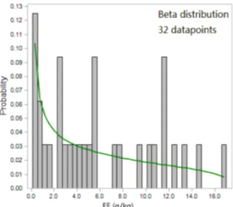
ern China, are excluded for EF analysis for southern provinces. For EFs with adequate domestic measurement data, a probability distribution is fitted using the statistical soft-ware package Crystal Ball and the Kolmogorov–Smirnov test for the goodness-of-fit
(p=0.05). As shown in Fig. 1, the OC EFs of crop wastes and bituminous chunk coal,
and EC EF of bituminous briquettes burned in stoves pass the test and their probability
15
distributions are presented. For EFs with insufficient observation data, and those that
fail to pass the goodness-of-fit test, probability distributions must be assumed follow-ing our previous work (Zhao et al., 2011). Detailed information on EC and OC EFs by source is summarized in Table 1.
For other sectors, few studies based on EC and/or OC EF measurement have been
20
published in recent years and the EFs summarized in Y. Zhao et al. (2013) are used in this study in most cases. For transportation, the results from on-road measurements by Huo et al. (2012), Wu et al. (2012) and Fu et al. (2013) are incorporated into the
emission factor database developed by Y. Zhao et al. (2013). The PM2.5 EF for
light-duty diesel trucks meeting stage I emission standards is updated from 3.4 to 2.3 g kg−1
25
and that for inland shipping from 1.1 to 2.2 g kg−1
ACPD
15, 8983–9032, 2015Patterns in atmospheric carbonaceous aerosols in China
H. Cui et al.
Title Page
Abstract Introduction
Conclusions References
Tables Figures
◭ ◮
◭ ◮
Back Close
Full Screen / Esc
Printer-friendly Version Interactive Discussion
Discussion
P
a
per
|
Discussion
P
a
per
|
Discussion
P
a
per
|
Discussion
P
a
per
|
2.3 Temporal trends, spatial distribution and uncertainties of emissions
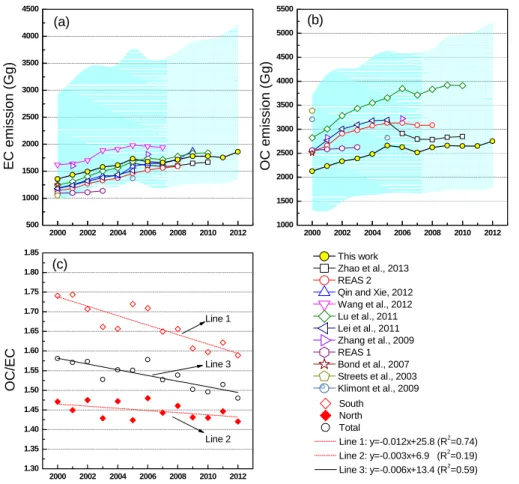
The calculated annual EC and OC emissions for 2000–2012 are presented in Fig. 2a and b, respectively. EC emissions are estimated to have increased by 37 % from 1356 Gg in 2000 to 1857 Gg in 2012, with relatively faster growth rates from 2000 to 2005 than the following years. Since 2005, improved emission control policies have
5
resulted in reduced PM emission factors on average that partly counteracted the ef-fects of increased activity levels. During the 2000–2012 research period, the
residen-tial sector is estimated to have accounted for 52±3 % of total EC emissions as an
annual average. The large contribution to total emissions is attributed mainly to
gen-erally inefficient combustion characteristics and a lack of effective emission controls in
10
this sector. During the period, emissions from the residential sector increased by 34 %, principally due to the growth of coal consumption. The shares of the industry and
trans-portation sectors are estimated at 32±2 %, and 16±2 %, respectively, while very little
emissions came from power plants because of the high combustion efficiency and
well-implemented particle controls. Emissions of industry and transportation increased by
15
39 and 47 %, much slower than the growth of activity data, namely 136 % in industrial coal consumption and 204 % in transportation oil consumption. This suggests improved emission control measures, e.g., the penetration of dust collectors with improved PM removal rates at industrial boilers, and the staged replacement of vehicles with stricter emission standards required by the national regulations.
20
OC emissions, shown in Fig. 2b, are estimated to have increased 29 % from 2127 Gg in 2000 to 2749 Gg in 2012, and the inter-annual trend is similar to that of EC emis-sions. Residential, industrial, and transportation sectors are estimated to have
con-tributed 76±2, 19±2, and 5±1 % to total emissions, respectively, and the emissions
of those sectors grew by 30, 25, and 39 % during the research period. In particular, the
25
share of emissions from biofuel use and biomass open burning is estimated at 58±3 %.
As shown in Fig. 2c, the ratios of OC to EC emissions, (OC/EC)emi, are estimated to
ACPD
15, 8983–9032, 2015Patterns in atmospheric carbonaceous aerosols in China
H. Cui et al.
Title Page
Abstract Introduction
Conclusions References
Tables Figures
◭ ◮
◭ ◮
Back Close
Full Screen / Esc
Printer-friendly Version Interactive Discussion
Discussion
P
a
per
|
Discussion
P
a
per
|
Discussion
P
a
per
|
Discussion
P
a
per
China (from 1.74 to 1.68) than northern China (from 1.47 to 1.42). The regional diff
er-ence in (OC/EC)emican be attributed mainly to different levels of biofuel and biomass
combustion, the sources with relatively high ratios of OC to EC emissions. These two sources are estimated to have contributed around 50 % to total OC emissions in north China, 66 % in the south. Moreover, some kinds of stoves that are commonly used for
5
heating in northern China, e.g., kangs, have lower OC to EC emission ratios than cook stoves, according to recent field measurements (Shen et al., 2010, 2013).
Relative changes in emissions of total primary carbonaceous aerosols (i.e., TC,
equal to OC+EC) between 2000 and 2012 are indicated by province in Fig. 3.
In contrast to most provinces where growth in primary TC emissions is found,
10
some economically-advanced provinces including Beijing in the JJJ region, Shang-hai, Jiangsu, and Zhejiang in the YRD region, and Guangdong in the PRD region, are estimated to have reduced their TC emissions during the last 10 years. The emission abatement in Beijing and Shanghai is attributed mainly to reduced energy consumption in the industrial sector, while that in Zhejiang and Jiangsu to reduced solid fuel use in
15
the residential sector. Both situations indicate gradually improving economic and en-ergy structures in the developed areas with relatively serious air pollution, and suggest increased attention to TC emission control in less economically advanced areas in the country. Shown in Fig. 3 as well are the emission intensities (i.e., emissions per unit territorial area) of TC by province in 2012, with the shares of OC and EC also indicated.
20
In the most densely populated provinces in eastern and central China, larger intensi-ties are generally found in the north than the south (provinces in the far north and west such as Xinjiang, Tibet, and Inner Mongolia are sparsely populated). In the populous and industrialized eastern part of the country, the annual average emission intensity of
primary TC for 2000 to 2012 is estimated at 1.30 metric tons km−2(t TC km−2) in
north-25
ern provinces (Beijing, Tianjin, Hebei, Henan, Jilin, Liaoning, Shaanxi, Shandong, and Shanxi), 33 % higher than that for southern provinces (Jiangsu, Anhui, Shanghai, Zhe-jiang, Chongqing, Fujian, Guangdong, Guangxi, Guizhou, Hubei, Hunan, and Jiangxi)
rea-ACPD
15, 8983–9032, 2015Patterns in atmospheric carbonaceous aerosols in China
H. Cui et al.
Title Page
Abstract Introduction
Conclusions References
Tables Figures
◭ ◮
◭ ◮
Back Close
Full Screen / Esc
Printer-friendly Version Interactive Discussion
Discussion
P
a
per
|
Discussion
P
a
per
|
Discussion
P
a
per
|
Discussion
P
a
per
|
son for different ambient concentrations of carbonaceous aerosols, as discussed later
in Sect. 3.1.
The uncertainties of emissions of EC and OC for each year are quantified with Monte-Carlo simulation as described in Zhao et al. (2011). Based on 10 000 simu-lations, the uncertainties of emissions, expressed as 95 % confidence intervals (CIs)
5
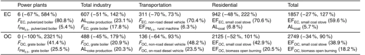
around the central estimates, and the parameters most significant in determining the uncertainties, judged by their contribution to the variance, are generated by sector. As shown in Table 2, the uncertainties of EC and OC emissions for 2012 are estimated
at−27 to 127 and−34 to 90 %, respectively, and no significant variation or clear
inter-annual trend is found for uncertainties of emissions for other years. The uncertainties
10
estimated in this work are smaller than previous work (Lu et al., 2011; Zhao et al., 2011; Y. Zhao et al., 2013). The decreased uncertainties mainly appear in the residential sec-tor and can be attributed to the updated emission facsec-tors that combine the most recent results from domestic field measurements. In most cases, the parameters associated with emission factors are estimated to contribute largest to the emission uncertainties,
15
with an exception of the industrial sector in which the coke production level is also significant. The total emissions, both for EC and OC, are most sensitive to the emis-sion factors of small coal stoves and crop waste burning, suggesting further work on emission characteristics for those sources.
2.4 Comparison with other emission inventory studies
20
The comparisons of EC and OC emissions from this work and other studies are shown in Fig. 2. Note emissions of forest and savanna burning are excluded from the total emissions provided by original studies. In general, estimates of most studies are within the uncertainties evaluated in this work, with the exception of EC emissions by the Regional Emission Inventory in Asia (REAS) version 1 (REAS 1, Ohara et al., 2007).
25
The inter-annual trends of EC emissions are in good agreement between studies, with
relatively steady growth rates during 2000–2005 and then leveling offfor the following
ACPD
15, 8983–9032, 2015Patterns in atmospheric carbonaceous aerosols in China
H. Cui et al.
Title Page
Abstract Introduction
Conclusions References
Tables Figures
◭ ◮
◭ ◮
Back Close
Full Screen / Esc
Printer-friendly Version Interactive Discussion
Discussion
P
a
per
|
Discussion
P
a
per
|
Discussion
P
a
per
|
Discussion
P
a
per
studies including Lei et al. (2011), Lu et al. (2011), Y. Zhao et al. (2011, 2013), Qin
and Xie (2012) and REAS 2 (Kurokawa et al., 2013). The differences can be attributed
to two reasons. First, some studies omitted some emission sources included here,
e.g., off-road vehicles (Klimont et al., 2009; Qin and Xie, 2012; Kurokawa et al., 2013),
biomass open burning (Lei et al., 2011; Kurokawa et al., 2013), and non-combustion
5
industrial processes (Kurokawa et al., 2013). Second, emission factors for residential coal combustion used in Lu et al. (2011), Lei et al. (2011) and REAS 2 are significantly lower than ours, which based on local measurements. EC emissions from 2005 to 2010 estimated in this work are a little higher than our previous work (Y. Zhao et al., 2013), because wood combustion in industry is now included and larger emission factors for
10
small coal and biofuel stoves are used in the current estimate. R. Wang et al. (2012) has the highest EC emission estimates among all the studies, due mainly to the higher emission factors of residential fuels used in that study.
Our estimates of OC emissions are roughly 1000 Gg lower than those of Lu et al. (2011), and 500 Gg lower than those of Zhang et al. (2009), Lei et al. (2011)
15
and REAS 2, even though they did not include the emissions from biomass open burn-ing, an important OC source that is estimated to contribute 400–600 Gg OC emissions per year according to Lu et al. (2011) and this work. The relatively big gaps between studies come mainly from the highly varied emission factors of residential biofuel
com-bustion used in different inventories. The OC emission factors for biofuel employed
20
by Lu et al. (2011), Zhang et al. (2009), Lei et al. (2011), and REAS 2 are almost twice ours. Those emission factors, however, were largely based on a review by Bond et al. (2004) with a global scope and were calculated as products of PM emission
fac-tors and mass fractions of carbonaceous species (i.e.,FEC and FOC) from laboratory
experiments, because no direct measurements of carbonaceous aerosol emission
fac-25
tors for cook stoves were available at that time,FEC and FOC for crop wastes burned
in cook stoves, for example, were estimated at 0.15 and 0.57, respectively, leading to a ratio of emission factors of OC and EC of 3.8. Nevertheless, the design and
ACPD
15, 8983–9032, 2015Patterns in atmospheric carbonaceous aerosols in China
H. Cui et al.
Title Page
Abstract Introduction
Conclusions References
Tables Figures
◭ ◮
◭ ◮
Back Close
Full Screen / Esc
Printer-friendly Version Interactive Discussion
Discussion
P
a
per
|
Discussion
P
a
per
|
Discussion
P
a
per
|
Discussion
P
a
per
|
countries (personal communication with Y. Chen from Yantai Institute of Coastal Zone Research, Chinese Academy of Sciences, 2014). Measurements of emission factors for biofuel burned in typical Chinese cook stoves have now gradually been conducted (Cao et al., 2008; Li et al., 2009; Shen et al., 2010, 2012, 2013; Wei et al., 2014).
In-corporating the results of these local studies, EFECdoes not differ much but the EFOC
5
to EFECratio for crop waste burning is estimated at 2.2, i.e., 45 % lower than that
sug-gested by Bond et al. (2004). Lower emission factors and thereby emissions of OC are thus estimated in this work compared to previous studies. Given the complexity of China’s residential stoves and possible huge variation of combustion conditions, how-ever, the representativeness and accuracy of existing measurements, and the emission
10
inventories based on those measurements, should continue to be carefully evaluated as more observations on pollution trends of carbonaceous aerosols become available.
3 Characteristics of carbonaceous aerosols based on observations
The temporal, spatial and size distributions of ambient carbonaceous aerosols are an-alyzed based on available data for China. A database of OC and EC concentrations
15
is compiled from literature on or including observation of carbonaceous aerosols over a recent 10 year period (2000–2010) in China. “Carbonaceous aerosol concentrations”
refers here to those in PM2.5, apart from discussion of size distribution in Sect. 3.4 and
where otherwise specifically noted. It is also acknowledged that comparison of OC and
EC concentrations in studies using different analytical methods introduces uncertainty.
20
Given the relatively large temporal and spatial scales concerned, we believe such un-certainty would not lead to significant statistical errors in this work.
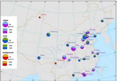
3.1 Spatial pattern of OC and EC levels
To better understand the spatial patterns of carbonaceous aerosol levels, OC and EC
concentrations reported in different regions across the country with sufficient sampling
ACPD
15, 8983–9032, 2015Patterns in atmospheric carbonaceous aerosols in China
H. Cui et al.
Title Page
Abstract Introduction
Conclusions References
Tables Figures
◭ ◮
◭ ◮
Back Close
Full Screen / Esc
Printer-friendly Version Interactive Discussion
Discussion
P
a
per
|
Discussion
P
a
per
|
Discussion
P
a
per
|
Discussion
P
a
per
periods (at least including both cold and warm seasons) were selected and summa-rized in Table S1 in the supplement. Studies with relatively short sampling periods are excluded. Geographical locations of the ground observation sites of the compiled data
are illustrated in Fig. S1 in the supplement. The sites can be classified into different
groups: urban/suburban sites located in/near large cities, rural sites that are more
rep-5
resentative for regional concentrations, and remote sites that are hardly influenced by human activities and thus representative for background concentrations.
Among the selected studies, the annual means of urban ambient concentrations
range from 7.1–64.8 µg m−3 for OC and 2.2–14.3 µg m−3 for EC, with an average of
20.2 and 6.1 µg m−3, respectively. From fewer studies, the averages of OC and EC
con-10
centrations for suburban sites are estimated at 17.4 and 4.2 µg m−3
, respectively, lower than those for urban sites. In general, those values are much higher than those of cities
in industrialized Asian countries, North America, and Europe. For example, 5.5 µg m−3
for OC and 3.1 µg m−3
for EC were observed at Saitama, Japan during July 2009–
April 2010 (Kim et al., 2011); 2.7 µg m−3 for OC and 1.1 µg m−3 for EC at New York
15
during February 2000–December 2003 (Qin et al., 2006); and 3.8 µg m−3 for OC and
3.8 µg m−3
for EC at Madrid during June 2009–February 2010 (Pio et al., 2011).
Par-ticularly high concentrations were found in Xi’an (64.8 µg m−3 for OC and 14.3 µg m−3
for EC in 2003) and Chongqing (50.9 µg m−3for OC and 12.3 µg m−3 for EC in 2003),
due probably to the combined contribution of coal combustion emissions and
unfa-20
vorable meteorological conditions (Cao et al., 2007). However, the average carbona-ceous concentrations measured by Chen et al. (2014) during May 2012–April 2013
in Chongqing (19 µg m−3 for OC and 4.6 µg m−3 for EC) were significantly lower than
those measured by Cao et al. (2007) in 2003, presumably due to improved implemen-tation of emission control polices. Compared with Xi’an, the relatively lower
concen-25
ACPD
15, 8983–9032, 2015Patterns in atmospheric carbonaceous aerosols in China
H. Cui et al.
Title Page
Abstract Introduction
Conclusions References
Tables Figures
◭ ◮
◭ ◮
Back Close
Full Screen / Esc
Printer-friendly Version Interactive Discussion
Discussion
P
a
per
|
Discussion
P
a
per
|
Discussion
P
a
per
|
Discussion
P
a
per
|
of OC and EC concentrations with ratios of observed OC to EC (OC/EC) of around
2.7, implying similar sources of carbonaceous aerosols and/or regional meteorological conditions. In addition, the concentrations of carbonaceous aerosols in China overall show a clear pattern, as Cao et al. (2007) investigated in 14 cities in 2003, with higher pollution levels found in northern and inland cities while lower levels found in
south-5
ern and coastal ones. The difference between north and south in China results partly
from (1) the larger emission intensity of primary carbonaceous aerosols in the north as described in Sect. 2.3, particularly in the heating seasons due to enhanced use of coal and biofuel in the residential sector (Lu et al., 2010); and (2) relatively favorable meteorological conditions including more frequent precipitation and less temperature
10
inversion in the south. The effects of monsoonal rainfall could also be a reason for lower
concentrations in coastal cities than inland ones.
The annual average OC and EC concentrations at rural stations range from 4.9–
20.2 µg m−3 and 0.8–4.3 µg m−3, with the overall average concentrations at 11.9 and
2.4 µg m−3, respectively. Most observed OC concentrations are below 16 µg m−3
ex-15
cept for Jinan, a city impacted by intensive coal use. All EC concentrations are below
5 µg m−3and much smaller than those at the urban/suburban sites. As with the urban
sites, the carbonaceous aerosol levels at rural sites are generally higher than those
in other parts of the world, e.g., 1.6 µg m−3 of OC and 0.61 µg m−3of EC at Egbert in
Canada during August 2005–November 2007 (Yang et al., 2011b), 3.8 µg m−3 of OC
20
and 1.3 µg m−3of EC at Cape Fuguei in Taiwan during 2003–2007 (Chou et al., 2010),
and 3.2 µg m−3of OC and 0.9 µg m−3of EC at West Midlands in the UK during
Novem-ber 2005–May 2006 (Harrison and Yin, 2008).
The annual OC and EC concentrations at remote sites range from 0.48–7.5 and
0.06–0.7 µg m−3, respectively, much lower than those in urban, suburban, and rural
25
sites, as expected. The background concentrations are comparable to the levels at
Sonnblick in the Austrian Alps, at 0.81 µg m−3 of OC and 0.07 µg m−3 of EC during
ACPD
15, 8983–9032, 2015Patterns in atmospheric carbonaceous aerosols in China
H. Cui et al.
Title Page
Abstract Introduction
Conclusions References
Tables Figures
◭ ◮
◭ ◮
Back Close
Full Screen / Esc
Printer-friendly Version Interactive Discussion
Discussion
P
a
per
|
Discussion
P
a
per
|
Discussion
P
a
per
|
Discussion
P
a
per
3.2 OC/EC and SOC formation levels across the country
As noted above, ambient OC is composed of POC emitted directly and SOC formed by
chemical reactions in the atmosphere. In general, an OC/EC ratio exceeding a
thresh-old of 2 is used to indicate the presence of secondary organic aerosols (Turpin and
Lim, 2001). As shown in Table S1, all of the annual mean OC/EC ratios are equal to
5
or above 2.0, implying the prevalence of SOC across the country. In addition to an-nual averages, OC and EC concentrations observed across the country for relatively short sampling periods (i.e., to be seasonally representative) from available studies
are compiled and included in the OC/EC analysis. Illustrated in Fig. 4a are the
av-erages of OC/EC ratios vs. EC concentrations with standard deviations at southern
10
(S, open symbols) and northern (N, solid symbols) remote, rural, suburban, and urban sites in China. In general, ambient EC concentrations in north are higher than those
in south, but larger OC/EC ratios are found in south, particularly for remote, rural and
suburban sites. The result is consistent with the spatial pattern of provincial emissions
shown in Fig. 2c, with the annual means of (OC/EC)emi calculated at 1.67 and 1.45
15
for southern and northern China respectively during 2000–2012. Besides emissions,
differences in the conditions for SOC formation contribute as well to the divergent
am-bient OC/EC ratios in the south and north, which will be discussed later in this section.
While EC levels indicating pollution from primary emissions are higher at urban sites,
larger ambient OC/EC ratios are found for remote and rural sites. As shown in Fig. 4b,
20
regression analyses are conducted for seasonal OC and EC concentrations classified
by functional zone (i.e., urban, suburban, rural and remote regions). Ratios of OC/EC
are larger than 1.0 for all data points, and a clear difference in OC/EC is found by
functional zone, with the regression slopes of seasonal mean concentrations at 2.92 for urban, 3.29 for suburban, 3.46 for rural, and 6.64 for remote sites.
25
The variation in OC/EC ratios by functional zone results from the joint effects of
ACPD
15, 8983–9032, 2015Patterns in atmospheric carbonaceous aerosols in China
H. Cui et al.
Title Page
Abstract Introduction
Conclusions References
Tables Figures
◭ ◮
◭ ◮
Back Close
Full Screen / Esc
Printer-friendly Version Interactive Discussion
Discussion
P
a
per
|
Discussion
P
a
per
|
Discussion
P
a
per
|
Discussion
P
a
per
|
coal combustion, and biomass burning at 1.1, 2.7, and 9.0, respectively. For urban areas of economically advanced cities in the JJJ and YRD regions, vehicles make a greater contribution to total carbonaceous emissions and local sources dominate
the composition of ambient carbonaceous aerosols, leading to smaller OC/EC. As
can be seen in Fig. 4b, most of the seasonal OC/EC ratios lower than 2 (below the
5
Y =2X line) were observed at urban sites. In rural areas, biomass combustion (with
larger primary OC/EC emission ratio) contributes more than it does in urban areas,
and the regional contribution of aged aerosols with higher SOC levels helps to elevate
the ambient OC/EC. Similarly, the highest OC/EC are found for the remote or high
mountain areas, attributed to the following: (1) those sites are far from anthropogenic
10
sources, especially those with relatively high emissions of EC (e.g., vehicles), (2) the formation and regional transport of SOC has increased the contribution to OC levels compared to urban areas, (3) the influence of natural sources is significantly higher at remote sites, with enhanced production of OC but very little EC; and (4) semi-volatile organic compounds tend to be condensed to particle OC in high mountain areas due
15
to the low temperature.
Lacking any direct analytical techniques to quantify POC or SOC concentrations, several indirect methods have been used to estimate the latter. One of the most used is the EC-tracer method due to its simplicity and data availability. The concentration of SOC can be calculated with Eq. (3):
20
SOC=OCtot−(OC/EC)min×EC (3)
where SOC is the secondary OC concentration; OCtot and EC are the observed
to-tal OC and EC concentrations, respectively; and (OC/EC)min is the lowest observed
OC/EC ratio that is assumed to represent (OC/EC)pri, the ratio of primary OC and EC
emissions with the contribution of SOC excluded (Castro et al., 1999).
25
The mass fractions of POC and SOC, estimated by individual studies in different
re-gions across the country are shown in Fig. 5. The spatial pattern of SOC/OC levels
ACPD
15, 8983–9032, 2015Patterns in atmospheric carbonaceous aerosols in China
H. Cui et al.
Title Page
Abstract Introduction
Conclusions References
Tables Figures
◭ ◮
◭ ◮
Back Close
Full Screen / Esc
Printer-friendly Version Interactive Discussion
Discussion
P
a
per
|
Discussion
P
a
per
|
Discussion
P
a
per
|
Discussion
P
a
per
of OC, indicating a large contribution of primary anthropogenic emissions. In contrast, higher mass fractions of SOC to OC are found in other cities, particularly those in southern China, due mainly to the favorable condition for SOC formation such as
rela-tively high temperature and sufficient sunlight. For all sites, SOC/OC at the remote and
rural sites is generally greater than those at urban sites. It thus confirms the formation
5
and transport of SOC at a regional scale, and could partly explain the discrepancies in
OC/EC by region.
It should be noted that the EC-tracer method has uncertainties. As a
semi-quantitative method, the determination of (OC/EC)pri is arbitrary and may vary
sig-nificantly depending on the observation. In urban Tianjin, for example, the estimated
10
SOC/OC in 2008 (62 %, Gu et al., 2010) was more than twice that of 2009 (28 %,
P. Zhao et al., 2013). Hu et al. (2012) modified the method by varying (OC/EC)pri
within a defensible range to obtain a series ofR2correlation coefficients between SOC
and EC. The best (OC/EC)pri can then be determined as the one corresponding to
the minimumR2, or when SOC is least correlated with EC. The improved method was
15
used to calculate the SOC concentration during the summer of 2006 in Guangzhou.
The (OC/EC)pri from the improved method showed strong agreement with the
regres-sion slope of OC to EC in the days when the pollution was mainly influenced by local
emissions, indicating that the errors from the subjectively determined OC/EC threshold
can be partly reduced (Hu et al., 2012).
20
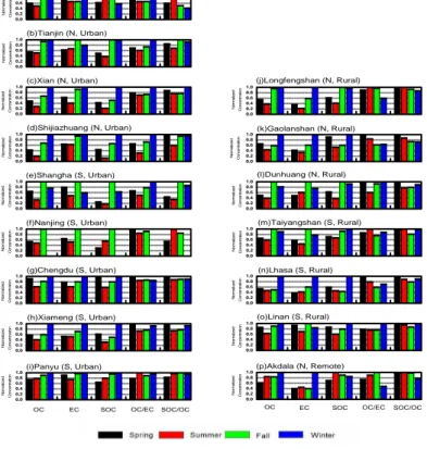
3.3 Seasonal variation of carbonaceous aerosol species
Seasonal variations of ambient carbonaceous aerosol levels are illustrated by region in Fig. 6. For ease of visualization, concentrations of OC, EC, and SOC for each season
are normalized by dividing by the maximum seasonal concentrations, while OC/EC
and SOC/OC are normalized by dividing by the maximum seasonal ratios.
25
concen-ACPD
15, 8983–9032, 2015Patterns in atmospheric carbonaceous aerosols in China
H. Cui et al.
Title Page
Abstract Introduction
Conclusions References
Tables Figures
◭ ◮
◭ ◮
Back Close
Full Screen / Esc
Printer-friendly Version Interactive Discussion
Discussion
P
a
per
|
Discussion
P
a
per
|
Discussion
P
a
per
|
Discussion
P
a
per
|
trations were found in autumn for Shanghai, probably due to the proximity of biomass combustion (Feng et al., 2009). In most cases, EC has the same seasonal pattern as OC, indicating they are of common origin and/or influenced by the same meteoro-logical factors. On the one hand, enhanced emissions (particularly in northern China) combined with a stagnant atmosphere favor accumulation in winter and result in an
5
increase of carbonaceous aerosol concentrations. On the other hand, the higher mixed layer and increased monsoonal precipitation in summer lead to stronger dispersion and
deposition of aerosols. Similar to OC and EC, OC/EC is generally higher in spring and
winter, whereas the seasonal variations in OC/EC at southern urban sites are
rela-tively small compared to those at northern sites, reflecting less difference in emissions
10
between cold and warm seasons in the south. Consistent seasonal patterns are found
between OC/EC and carbonaceous aerosol concentrations at northern urban sites,
while some inconsistencies, such as enhanced OC/EC in summer, occur in the south.
It thus implies that the meteorology that favors SOC generation may play a more im-portant role in the seasonal pattern of ambient carbonaceous aerosol levels and their
15
ratios in south.
As a component of OC, SOC concentrations are generally higher in autumn and winter except for Beijing (Lin et al., 2009) and Akdala (Qu et al., 2009), and similar seasonal variations are found for urban and rural sites. Despite the presence of more photochemical oxidants and VOC emissions in summer, the highest SOC
concentra-20
tions were observed in winter for most cities. The SOC level in winter in Shijiazhuang, for example, was notably 8 times higher than that in summer (P. Zhao et al., 2013). The stagnant conditions and low temperatures that facilitate the accumulation of air pollutants and accelerate the condensation or adsorption of VOC could be one rea-son for the high SOC in cold searea-sons (P. Zhao et al., 2013). Using a smog chamber
25
ACPD
15, 8983–9032, 2015Patterns in atmospheric carbonaceous aerosols in China
H. Cui et al.
Title Page
Abstract Introduction
Conclusions References
Tables Figures
◭ ◮
◭ ◮
Back Close
Full Screen / Esc
Printer-friendly Version Interactive Discussion
Discussion
P
a
per
|
Discussion
P
a
per
|
Discussion
P
a
per
|
Discussion
P
a
per
formation, estimated to be responsible for 44–71 % of total OC in four big cities across China (Huang et al., 2014).
A larger contribution of SOC to OC (SOC/OC) is found in fall and winter for most
sites, while its seasonal variations are generally smaller compared to those of SOC concentrations, particularly for rural, remote, and southern urban sites. The highest
5
SOC/OC ratios were in fact found in summer at some urban sites including Beijing
(Lin et al., 2009), Nanjing (Wu et al., 2013; Li et al., 2015) and Tianjin (Gu et al., 2010, not plotted in Fig. 6), and rural or remote sites such as Longfengshan, Taiyangshan and Akdala (X. Zhang et al., 2008, 2012). Although the absolute SOC levels are higher in winter, the oxidation reactions from VOC to OC are implied to be faster in summer
10
because of higher temperature and more abundant VOC precursors, accelerating SOC
formation and thus elevating SOC/OC.
3.4 Distribution of carbonaceous species by particle size
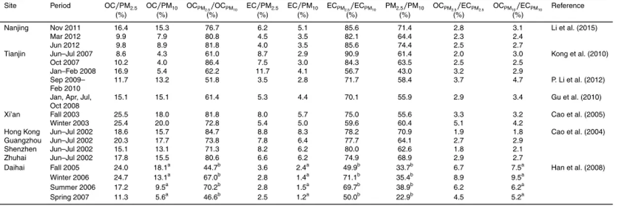
The relationships of ambient OC, EC, and the OC/EC ratio to different particle sizes
are given in Table 3. From available observations, the OC and EC mass fractions of
15
fine particles (PM2.5) (8.6–25.5 and 3.5–11.7 %, respectively) are larger than those of
PM10 (4.0–20.0 and 2.8–8.3 %). The OC and EC mass in PM2.5respectively accounts
for 51.8–86.4 and 56.7–90.9 % of that in PM10, greater than the mass fractions of PM2.5
to PM10(43.0–74.4 %). This information clearly confirms that ambient OC and EC are
not uniformly distributed in particles but enriched in the fine particle fraction. Larger
20
OC/EC ratios, however, are found in PM10 than in PM2.5 in most cases. Such diff
er-ing distributions of OC and EC reflect the different sources of carbonaceous aerosols
in the atmosphere (G. Wang et al., 2010). EC is usually associated with incomplete combustion, which releases into the atmosphere carbonaceous matter mainly in the form of submicron particles. Also enriched in fine particles, OC is nevertheless
dis-25
ACPD
15, 8983–9032, 2015Patterns in atmospheric carbonaceous aerosols in China
H. Cui et al.
Title Page
Abstract Introduction
Conclusions References
Tables Figures
◭ ◮
◭ ◮
Back Close
Full Screen / Esc
Printer-friendly Version Interactive Discussion
Discussion
P
a
per
|
Discussion
P
a
per
|
Discussion
P
a
per
|
Discussion
P
a
per
|
(Matthias-Maser and Jaenicke, 2000). Therefore, the smaller OC/EC ratios in PM2.5
imply a greater importance of anthropogenic sources to fine particles. The results in
China are consistent with European studies, in which OC/EC in cities was higher in
larger particles (Pio et al., 2011).
3.5 Characteristics of carbonaceous aerosols for typical periods
5
In addition to research focused on annual or seasonal averages, studies have been conducted on carbonaceous aerosol levels during high-pollution, clear, and other typ-ical event periods. For example, at a rural site in the PRD in summer of 2006, the average OC and EC concentrations observed during days of strong influence of local emissions or of typhoons and high precipitation compared to normal days (Hu et al.,
10
2012). Clear distinctions in pollution levels were found between periods: 28.1 µg m−3
of
OC and 11.6 µg m−3 of EC during days of strong local emission influence; 4.0 µg m−3
of OC and 1.8 µg m−3of EC during those influenced by typhoons or high precipitation;
and 5.7 µg m−3
of OC and 3.3 µg m−3
of EC for normal days. Relatively low concen-trations of carbonaceous aerosols were observed during the campaigns of the Beijing
15
Olympics in 2008 (X. Li et al., 2012), Shanghai World Expo in 2010 (Wang et al., 2014),
and Nanjing Asian Youth Games in 2013 (Yu et al., 2014), showing the effectiveness of
pollution control measures on air quality for those events.
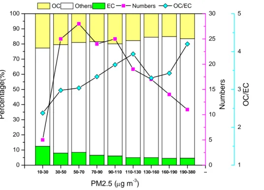
More studies have focused on heavy pollution periods, such as hazy days and biomass burning seasons. A hazy day is defined by daily average atmospheric
visi-20
bility less than 10 km (Hou et al., 2011), with PM2.5one of the most important
contribu-tors. In this work, the seasonal averages of PM2.5concentrations in urban or suburban
sites throughout China during 2000–2010 are compiled based on available studies,
and an approximate lognormal distribution is derived for frequency of PM2.5levels with
a data sample size of 170, as shown in Fig. 7. Around 60 % of the PM2.5 values
ex-25
ceeded the national standard of 75 µg m−3
ACPD
15, 8983–9032, 2015Patterns in atmospheric carbonaceous aerosols in China
H. Cui et al.
Title Page
Abstract Introduction
Conclusions References
Tables Figures
◭ ◮
◭ ◮
Back Close
Full Screen / Esc
Printer-friendly Version Interactive Discussion
Discussion
P
a
per
|
Discussion
P
a
per
|
Discussion
P
a
per
|
Discussion
P
a
per
other components in PM2.5were greatly enhanced during local haze periods, by up to
430 % in Guangzhou (Jung et al., 2009) and about 160, 170, and 180 % for OC, EC and secondary non-organic aerosols (SNA), respectively, in Fuzhou (F. Zhang et al., 2013). As shown in Fig. 7, moreover, larger mass fractions of carbonaceous aerosols
in PM2.5 are found for periods with relatively lower PM2.5 levels, and the fractions of
5
OC and EC to PM2.5 were 27 and 63 % less, respectively, at PM2.5 concentrations
of 190–380 µg m−3 compared to those of 10–30 µg m−3. The results indicate, on one
hand, that rapid increase in other compounds like SNA contribute significantly to heavy haze events. For example, in Beijing, the fraction of particles composed of inorganic
ions (SO24−+NO−3+NH+4) increased as PM2.5levels rose during 1999–2010 (data
pro-10
vided by K. He of Tsinghua University, 2012). On the other hand, the sharp increase
in OC/EC along with enhanced PM2.5 levels indicates significant contribution of SOC
to strong haze events. For example, Huang et al. (2011) found that hazy episodes in Harbin were closely related to the high concentrations of OC and EC, and the
aver-age OC/EC ratio on hazy days (42.2) was almost three times of that in non-haze days
15
(14.5).
Biomass burning is another source with significant impact on ambient aerosol levels and air quality. Elevated levels of carbonaceous aerosols were usually found during the harvest season. For example, OC and EC were observed to increase by 99 and 105 %, respectively, during the biomass-burning vs. non-biomass-burning periods in
20
Guangzhou (Zhang et al., 2010), and the analogous values for Chengdu were ob-served to be 148 and 51 % (Wang et al., 2013). With other methods combined, the biomass-burning share of carbonaceous aerosol enhancement has also been quan-tified in recent studies. Li et al. (2015), using regression analysis of particle OC and
K+ of biomass burning origin, estimated that biomass burning contributed more than
25
half of ambient OC during the harvest season in Nanjing. Based on observations and chemical transport modeling, Cheng et al. (2014) estimated that open biomass burning
ACPD
15, 8983–9032, 2015Patterns in atmospheric carbonaceous aerosols in China
H. Cui et al.
Title Page
Abstract Introduction
Conclusions References
Tables Figures
◭ ◮
◭ ◮
Back Close
Full Screen / Esc
Printer-friendly Version Interactive Discussion
Discussion
P
a
per
|
Discussion
P
a
per
|
Discussion
P
a
per
|
Discussion
P
a
per
|
the YRD region during May and June, and that a complete ban of biomass burning
would reduce the human exposure level of PM2.5in the region 47 %.
4 Assessment of emission inventories using observations
4.1 Comparisons of inter-annual trends in ambient levels and emissions for
2000–2010 5
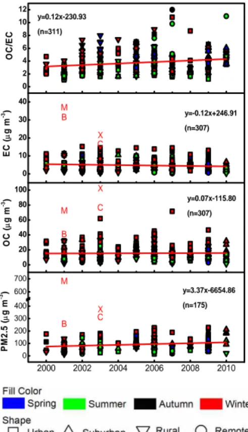
The seasonal means of OC, EC, and PM2.5 concentrations and the ratios of OC to
EC based on available observations are plotted from 2000 to 2010 in Fig. 8, to re-flect the trends of carbonaceous aerosols at the national scale. Although an increasing inter-annual trend is found for estimated OC and EC emissions over the 10 years, the observed concentrations of carbonaceous aerosols did not likewise increase, and
ob-10
served EC actually declined. On the one hand, the improvement of fuel combustion technologies in the residential sector and thereby the possible changes in emission factors cannot be fully captured in current emission inventory studies because of insuf-ficient data on key parameters. This may result in overestimated growth of emissions than indicated by observed concentrations. Databases of evolving emission factors
15
over time reflecting incremental emission control, particularly in residential combus-tion sources, are necessary to improve understanding of long-term emission trends in China. On the other hand, the ambient levels of carbonaceous aerosols could also be influenced by changes in meteorological factors in air quality, including wind veloc-ity, humidveloc-ity, temperature, and stability of the atmosphere (J. Wang et al., 2012). For
20
example, divergent trends in local meteorology for the JJJ and PRD regions led to op-posite trends in carbonaceous aerosol levels for the two regions (increased in JJJ but decreased in PRD) in recent years (X. Zhang et al., 2013). The estimates of emissions by region should thus be improved to incorporate detailed information on local sources,
to carefully differentiate the impacts of emissions and meteorology on carbonaceous
25
ACPD
15, 8983–9032, 2015Patterns in atmospheric carbonaceous aerosols in China
H. Cui et al.
Title Page
Abstract Introduction
Conclusions References
Tables Figures
◭ ◮
◭ ◮
Back Close
Full Screen / Esc
Printer-friendly Version Interactive Discussion
Discussion
P
a
per
|
Discussion
P
a
per
|
Discussion
P
a
per
|
Discussion
P
a
per
Observations indicate increased OC/EC ratios from 2000 to 2010 at the national
scale (Fig. 8), but emission inventories indicate slightly reduced ratios (from 1.58 in 2000 to 1.48 in 2010, as shown in Fig. 2c). This inconsistency might result from (1) the possible underestimate of emissions from sources with significant primary OC, e.g., biomass burning (described later in Sect. 4.2), and (2) enhanced SOC formation from
5
increasing VOC emissions (Bo et al., 2008; Wei, 2009) and elevated atmospheric
oxi-dation. For comparison, primary PM2.5emissions are estimated to have declined after
2005, due to the improved energy structure and emission controls in certain
indus-trial sources and transportation (Y. Zhao et al., 2013), while PM2.5concentrations have
been increasing in recent years (Fig. 8). The result emphasizes that the ambient PM2.5
10
level is not only determined by primary particle emissions, and that secondary parti-cle formation driven by emissions of precursors and enhanced atmospheric oxidation appears to be playing increasingly important roles in PM pollution across the country.
4.2 Evaluation of emission inventories based on the (OC/EC)pri
The validity of current emission inventories of carbonaceous aerosols is evaluated
15
through available observations of OC/EC ratios. The following criteria are used to
se-lect observational data: (1) observation sites must be located in rural or remote areas that are more representative of regional pollution from emissions, (2) the ratio of
pri-mary OC and EC, (OC/EC)pri, must be provided or can be calculated based on the
observations; and (3) the sampling period must be sufficient for evaluation of annual
20
emissions. With these restrictions, the observational data suitable for (OC/EC)pri
eval-uation come mainly from X. Zhang et al. (2008) for 2006. As shown in Fig. 9, the value
of (OC/EC)pri from given observational sites is indicated on thex axis, while that from
the estimated emissions for the province where the site is located is shown on the
y axis. The correlations of (OC/EC)pri between observations and emissions are then
25
ACPD
15, 8983–9032, 2015Patterns in atmospheric carbonaceous aerosols in China
H. Cui et al.
Title Page
Abstract Introduction
Conclusions References
Tables Figures
◭ ◮
◭ ◮
Back Close
Full Screen / Esc
Printer-friendly Version Interactive Discussion
Discussion
P
a
per
|
Discussion
P
a
per
|
Discussion
P
a
per
|
Discussion
P
a
per
|
inventories do not include emissions from open burning of biomass, we corrected their results by adding that part of emissions calculated by this work to their original totals.
As can be seen in Fig. 9, the data points based on provincial emissions estimated by
this work, with a regression slope of 0.97, are in best agreement with theY =X line,
while the emission ratios [(OC/EC)emi] of the other inventories are 20–50 % higher
5
than the observed concentration ratios. The residual sum of squares (RSS), which measures the discrepancy of the data and the linear regression model, is calculated as well for all the inventories, and the lowest RSS (and thereby random error) is found for this work, at 1.18. The comparison thus indicates improved reliability and reduced un-certainty of our inventory, resulting largely from a more detailed classification of source
10
categories and application of emission factors from local field measurements. It should
be noted that the (OC/EC)priobtained from observations in Nanning is much lower than
(OC/EC)emifor its province, Guangxi, estimated in this work (point A in Fig. 9). The
de-viation might result partly from the fact that the observation was actually conducted in an urban area but categorized as a rural measurement because of less intense
emis-15
sion activity in this relatively underdeveloped city, according to X. Zhang et al. (2008). It thus further implies the better representativeness of regional emission levels by obser-vation at rural or remote sites. Excluding point A from the linear regressions analysis, the slope comparing the observations and emissions estimated by this work would change to 0.92, with an SSR reduced to 0.62, while those for Zhang et al. (2009), Lei
20
et al. (2011) and REAS 2 are recalculated as 1.12, 1.27 and 1.35, with SSRs of 1.58, 1.36 and 2.60, respectively (not shown in Fig. 9).
Despite efforts to improve the emission estimation, the regression slopes
compar-ing OC/EC from emissions in this work to observations are less than 1.0. In
particu-lar, (OC/EC)pri obtained from observations at two sites, Longfengshan in Heilongjiang
25
(point B) and Taiyangshan in Hunan (point C) are clearly larger than (OC/EC)emi in
this work, but closer to those for other inventories. This deviation thus implies a
pos-sible underestimate of emissions for sources with high OC/EC ratio, e.g., combustion
ACPD
15, 8983–9032, 2015Patterns in atmospheric carbonaceous aerosols in China
H. Cui et al.
Title Page
Abstract Introduction
Conclusions References
Tables Figures
◭ ◮
◭ ◮
Back Close
Full Screen / Esc
Printer-friendly Version Interactive Discussion
Discussion
P
a
per
|
Discussion
P
a
per
|
Discussion
P
a
per
|
Discussion
P
a
per
uncertainty comes from a lack of sufficient evaluation of the representativeness and
re-liability of emission factors of biofuel use from limited domestic measurements. Another important reason for the relatively low OC emission results could be possible underes-timation of biomass open burning in some areas. In the bottom-up method, the amount of biomass burning in clear fields depends significantly on one parameter: the ratio
5
of burned crop wastes to the total produced. Existing investigations of this ratio, with
its spatial distribution and temporal trends across the country, are far from sufficient,
and piecemeal information from local government plans on renewable energy or con-stant values from individual surveys (e.g., Wang and Zhang, 2008) have to be applied
in emission estimation, though they likely differ significantly from facts on the ground.
10
For example, increased ratios of crop waste recycling and utilization (which imply de-creased ratios of crop wastes burned in open fields) are suggested in the government plans from 2005 to 2012 in the YRD region, where the air quality is influenced heav-ily by open biomass burning in harvest season. According to fire counts and intensity observed by satellite with MODIS (Moderate Resolution Imaging Spectroradiometer,
15
https://earthdata.nasa.gov/data/near-real-time-data/firms), however, a growing trend of biomass burning is found for the region during the period (X. Huang et al., 2012; Yang et al., 2015). Moreover, relatively strong signals of fire intensity are indicated by MODIS for northeastern and south-central China, close to the observation sites of points B and C in Fig. 9, respectively, implying considerable influence of biomass
burn-20
ing on the ambient carbonaceous aerosol levels in those regions. To better understand the levels and trends of carbonaceous aerosol emissions in China, therefore, more ob-servations from ground sites and satellites should be collected and incorporated into the framework of bottom-up emission estimation methods.
5 Conclusions
25