www.atmos-chem-phys.net/15/8201/2015/ doi:10.5194/acp-15-8201-2015
© Author(s) 2015. CC Attribution 3.0 License.
Climate responses to anthropogenic emissions of short-lived
climate pollutants
L. H. Baker1, W. J. Collins1, D. J. L. Olivié2, R. Cherian3, Ø. Hodnebrog4, G. Myhre4, and J. Quaas3 1Department of Meteorology, University of Reading, P.O. Box 243, Reading, RG6 6BB, UK
2Norwegian Meteorological Institute, Oslo, Norway
3Institute for Meteorology, University of Leipzig, Leipzig, Germany
4Center for International Climate and Environmental Research – Oslo (CICERO), Oslo, Norway
Correspondence to:L. H. Baker ([email protected])
Received: 22 December 2014 – Published in Atmos. Chem. Phys. Discuss.: 10 February 2015 Revised: 3 June 2015 – Accepted: 1 July 2015 – Published: 24 July 2015
Abstract.Policies to control air quality focus on mitigating emissions of aerosols and their precursors, and other short-lived climate pollutants (SLCPs). On a local scale, these poli-cies will have beneficial impacts on health and crop yields, by reducing particulate matter (PM) and surface ozone con-centrations; however, the climate impacts of reducing emis-sions of SLCPs are less straightforward to predict. In this pa-per we consider a set of idealized, extreme mitigation strate-gies, in which the total anthropogenic emissions of individual SLCP emissions species are removed. This provides an up-per bound on the potential climate impacts of such air quality strategies.
We focus on evaluating the climate responses to changes in anthropogenic emissions of aerosol precursor species: black carbon (BC), organic carbon (OC) and sulphur dioxide (SO2). We perform climate integrations with four fully cou-pled atmosphere–ocean global climate models (AOGCMs), and examine the effects on global and regional climate of re-moving the total land-based anthropogenic emissions of each of the three aerosol precursor species.
We find that the SO2 emissions reductions lead to the strongest response, with all models showing an increase in surface temperature focussed in the Northern Hemisphere mid and (especially) high latitudes, and showing a corre-sponding increase in global mean precipitation. Changes in precipitation patterns are driven mostly by a northward shift in the ITCZ (Intertropical Convergence Zone), consistent with the hemispherically asymmetric warming pattern driven by the emissions changes. The BC and OC emissions re-ductions give a much weaker response, and there is some
disagreement between models in the sign of the climate re-sponses to these perturbations. These differences between models are due largely to natural variability in sea-ice ex-tent, circulation patterns and cloud changes. This large natu-ral variability component to the signal when the ocean circu-lation and sea-ice are free-running means that the BC and OC mitigation measures do not necessarily lead to a discernible climate response.
1 Introduction
homoge-neous as in the case of WMGHGs, and concentrations tend to be highest nearer to source regions. Therefore the result-ing forcresult-ing patterns are also inhomogeneous, and diagnosresult-ing the regional and global climate impacts is much more com-plex than for WMGHGs (Shindell et al., 2009; Shindell and Faluvegi, 2009). In particular the majority of anthropogenic emissions of SLCPs are in the Northern Hemisphere, so the forcing is much stronger in the Northern Hemisphere than the Southern Hemisphere hemisphere (Shindell, 2014). The aerosol–radiation interactions and aerosol–cloud interactions bring further inhomogeneities, so the resulting impacts of SLCPs on regional and global climate are quite different to those for the WMGHGs.
In this paper we focus on aerosol and aerosol precursor emissions, namely black carbon (BC), organic carbon (OC) and sulphur dioxide (SO2), which is a precursor to sulphate (SO4) aerosol formation.
The effects of anthropogenic aerosols on climate are com-plex. Scattering aerosols (such as SO4and OC) reflect down-welling solar radiation back out of the atmosphere, result-ing in a negative top-of-atmosphere (TOA) short-wave (SW) forcing. This reduction in the solar radiation absorbed by the climate system results in a decrease in global mean sur-face temperature. Hydrophilic aerosols also provide cloud condensation nuclei (CCN), allowing more smaller cloud droplets to form, which increases the cloud albedo and the cloud amount, and prolongs the cloud lifetime by inhibiting precipitation. This further contributes to the negative forcing (Boucher et al., 2013). In contrast, BC aerosol absorbs in-coming solar radiation, which means it has a net warming ef-fect on the atmosphere and gives a positive TOA SW forcing. The local impact of BC on the surface temperature is depen-dent on the altitude of the BC: low-level BC can warm the surface by re-emitting radiation in the thermal wavelengths, whereas higher-level BC can reduce the surface tempera-ture by absorbing part of the downwelling solar radiation before it reaches the surface (Ramanathan and Carmichael, 2008). Even in cases where the surface is cooled locally, the additional solar radiation absorbed by the BC results in a warming effect on the higher atmosphere. BC located near to clouds can cause evaporation of clouds, known as the semi-direct effects (Koch and Del Genio, 2010). However, depend-ing on the exact location of the BC and type of cloud, BC can either increase or decrease cloud cover via various dif-ferent mechanisms (Ban-Weiss et al., 2012), so the net im-pact on clouds of a given atmospheric distribution of BC is highly complex. BC aloft causes stabilization of the atmo-sphere, which can lead to increased stratocumulous clouds (Koch and Del Genio, 2010). BC also has important impacts at high latitudes when it is deposited on snow, as it decreases the albedo of the snow surface (Ramanathan and Carmichael, 2008), and can enhance snowmelt by absorbing solar radia-tion after it is deposited (Flanner et al., 2007). However, the impacts of BC forcing in the Arctic on surface temperature are complex, as the result is highly dependent on the altitude
and location of the forcing (Sand et al., 2013a, b; Flanner, 2013).
Aerosols also affect precipitation (e.g. Kristjánsson et al., 2005; Ming et al., 2010; Boucher et al., 2013; Osborne and Lambert, 2014). On a global scale, we might expect the pre-cipitation to change in proportion to a given global temper-ature change driven by aerosol forcing, due to the increased amount of water vapour that the atmosphere can hold (Lam-bert and Webb, 2008). However, since the direct, semi-direct and indirect effects of aerosols will change precipitation pat-terns, this does not necessarily hold locally. Hydrophilic aerosol species can reduce precipitation locally, by enhanc-ing cloud droplet nucleation, which allows more smaller cloud droplets to form but inhibits the amount of droplets that become large enough to form precipitation. Other ef-fects such as convective invigoration that might also affect precipitation (Rosenfeld et al., 2008) are not parameterized in the models assessed here. BC has more complex effects on precipitation patterns since it warms the atmosphere (An-drews et al., 2010) but can either warm or cool the surface, which will increase or reduce the amount of surface evapo-ration and resulting precipitation (Ming et al., 2010). The net effect on precipitation is therefore dependent on the region and vertical profile of the BC aerosol (Andrews et al., 2010; Ban-Weiss et al., 2012; Kvalevåg et al., 2013). Furthermore the hemispherically asymmetric forcing from anthropogenic aerosol emissions impacts the temperature in the Northern Hemisphere more than in the Southern Hemisphere, lead-ing to a meridional shift in the Intertropical Convergence Zone (ITCZ) towards the warmer hemisphere (e.g. Kang et al., 2008; Ceppi et al., 2013; Hwang et al., 2013), which will impact local precipitation in the tropics and the mon-soon regions (Ming and Ramaswamy, 2009). Several stud-ies have shown that anthropogenic aerosol emissions in re-cent decades have contributed to the weakening of the North-ern Hemisphere monsoon (e.g. Bollasina et al., 2011; Polson et al., 2014). Aerosols also impact the hydrological cycle by reducing the amount of solar radiation reaching the surface, a process known as solar dimming (Gedney et al., 2014). Solar dimming acts to reduce evaporation, and results in increased run-off and suppressed evapotranspiration.
Here we assess the climate impacts of removing the to-tal land-based anthropogenic emissions of each of SO2, OC and BC in three coupled climate models (four models for the BC experiments) with interactive chemistry and aerosols. The multi-model nature of this work gives greater confidence in the results since we are not drawing conclusions based on results from just one model. The 100 % perturbations were used in order to achieve a strong enough forcing signal. Re-sults from atmosphere-only simulations (e.g. Bellouin et al., 2015) suggest that the removal of anthropogenic SO2and OC emissions will lead to a positive forcing and a global temper-ature increase, while removing anthropogenic BC emissions will lead to a negative forcing and a global temperature de-crease. Using coupled models allows the ocean circulation and heat uptake, and sea-ice extent, to respond to the atmo-spheric changes from the emissions perturbations. We assess the resulting changes in temperature and precipitation both globally and regionally.
In Sect. 2, the climate models, experimental setup and emissions data sets are described. In Sect. 3 the climate im-pacts of removing the emissions of individual anthropogenic aerosol species are presented. These results are discussed fur-ther in Sect. 4, and conclusions are given in Sect. 5.
2 Methodology
2.1 Description of models
The three main models used are HadGEM3, ECHAM6-HAM2 and NorESM1-M. HadGEM3 and NorESM1-M have interactive aerosols and chemistry; ECHAM6-HAM2 has in-teractive aerosols but does not include inin-teractive chemistry. Therefore in HadGEM3 and NorESM1-M, changes in the aerosols can affect the chemistry via changes in oxidation of SO2and changing the available surface for heterogeneous chemistry; these processes will directly and indirectly affect O3and OH. Photolysis is not affected by the aerosols in these models. The fact that ECHAM6-HAM2 does not include in-teractive chemistry is expected to lead to only minor differ-ences from the other two models with interactive chemistry with regard to the radiative and climate effects of aerosol and aerosol precursor emissions. For the BC perturbation experiments some additional simulations were performed: one extra ensemble member was run by each of HadGEM3 and NorESM1-M, and three ensemble members were run by NCAR CESM 1.0.4/CAM4. The extra BC simulations were included in order to explore the BC results further, as this work was part of a larger project of which BC was a key focus.
HadGEM3 is the Hadley Centre Global Environment Model version 3 (Hewitt et al., 2011). The atmosphere com-ponent has a horizontal resolution of 1.875◦×1.25◦and 85
vertical levels extending to 85 km in height (of which 50 are below 18 km). The atmosphere is coupled to the NEMO
ocean modelling framework with a horizontal resolution of 1.0◦ and 75 vertical levels, and to the CICE sea-ice model
(Hunke and Lipscomb, 2008). The UKCA TropIsop scheme is used to model gas-phase chemistry in the troposphere. This treats 55 chemical species (37 of which are transported) in-cluding hydrocarbons up to propane, and isoprene and its degradation products (O’Connor et al., 2014). Atmospheric gas and aerosol tracers are advected using the same semi-Lagrangian advection scheme as used for the physical cli-mate variables. Parameterized transport such as boundary layer mixing and convection is also as used for the physi-cal climate variables. Aerosols are modelled by the UKCA GLOMAP-mode aerosol scheme (Mann et al., 2010; Abdul-Razzak and Ghan, 2000). This models the internal mixing of SO4, OC, BC, dust and sea-salt using a two-moment modal approach and dynamically evolving particle size distribu-tions. There are seven modes: four soluble (nucleation to coarse) and three insoluble (Aitken to coarse). Aerosol pro-cesses are simulated in a size-resolved manner, including pri-mary emissions, secondary particle formation by binary ho-mogeneous nucleation of sulphuric acid and water, particle growth by coagulation, condensation, and cloud-processing, and removal by dry deposition, in-cloud and below-cloud scavenging. The effects of aerosols on clouds are modelled using an aerosol activation parameterization scheme (Abdul-Razzak and Ghan, 2002). The radiative impact from aerosols is calculated using the Edwards–Slingo radiation scheme (Edwards and Slingo, 1996).
ECHAM6-HAM2 is the European Centre for Medium-Range Weather Forecasts Hamburg model version 6 (Stevens et al., 2013). The atmospheric simulations were made us-ing the ECHAM6 GCM with a horizontal resolution of T63 (about 1.8◦×1.8◦) and a vertical resolution of 47
lev-els (extending from the surface to 0.01 hPa). The atmo-spheric model is coupled to the Max Planck Institute Global Ocean/Sea-Ice Model (MPIOM) with a bipolar grid with 1.5◦
resolution (near the equator) and 40 vertical levels (Jungclaus et al., 2013). The atmospheric model is extended with the Hamburg aerosol model (HAM2) version 2 (Zhang et al., 2012). The main components of HAM are the microphysi-cal module M7, which predicts the evolution of an ensem-ble of seven internally mixed lognormal aerosol modes (Vi-gnati et al., 2004), an emission module, a sulfate chemistry scheme (Feichter et al., 1996), a deposition module, and a radiative transfer module (Stier et al., 2005) to account for sources, transport, and sinks of aerosols as well as their ra-diative impact. Five aerosol components, namely SO4, OC, BC, sea-salt, and mineral dust, are considered in this model. Aerosol effects on liquid-water and ice clouds are considered following Lohmann et al. (2007). Oxidant fields for the sul-phate aerosol production were a 2003–2010 average from the MACC reanalysis (Inness et al., 2013).
lev-els in the vertical with a hybrid sigma pressure coordinate and model top at 2.19 hPa. The ocean module is an up-dated version of the isopycnic ocean model MICOM (with a 1.1◦resolution near the equator and 53 layers), while the sea-ice (CICE4) and land (CLM4) models and the coupler (CPL7) are basically the same as in CCSM4 (Gent et al., 2011). The atmosphere module CAM4-Oslo (Kirkevåg et al., 2013) is a version of CAM4 (Neale et al., 2011, 2013) with advanced representation of aerosols, aerosol–radiation and aerosol–cloud interactions. It uses the finite volume dy-namical core for transport calculations. CAM4-Oslo calcu-lates mass-concentrations of aerosol species that are tagged according to production mechanisms in clear and cloudy air and four size classes (nucleation, Aitken, accumulation, and coarse modes). These processes are primary emission, gaseous and aqueous chemistry (cloud processing), nucle-ation, condensnucle-ation, and coagulation. Loss terms are dry de-position, in-cloud and below-cloud scavenging. The aerosol components included are SO4, BC, organic matter (OM), sea-salt, and mineral dust, and are described by 20 tracers. In the model version used in this study, the aerosol mod-ule of CAM4-Oslo is coupled with the tropospheric gas-phase chemistry from MOZART (Emmons et al., 2010), which treats around 80 gaseous species. This coupling al-lows for a more explicit description of the formation of sec-ondary aerosol (SO4and secondary OM). The radiative forc-ing from aerosols is calculated usforc-ing the Collins (2001) ra-diation scheme. In the fully coupled NorESM1-M, albedo-effects of BC and mineral dust aerosols deposited on snow and sea-ice are also taken into account; this process is not represented in the other three models.
An additional model, NCAR CESM 1.0.4/CAM4, was used for the BC analysis only. NCAR CESM 1.0.4/CAM4 is the National Center for Atmospheric Research Community Earth System Model (Gent et al., 2011) run with the Com-munity Atmosphere Model version 4 (Neale et al., 2011). The atmospheric component is set up here with a horizon-tal resolution of 1.9◦×2.5◦, and 26 vertical layers
(extend-ing from the surface to 2.19 hPa). CAM4 is coupled to a full ocean model (Danabasoglu et al., 2012), which is based on the Parallel Ocean Program version 2 (Smith et al., 2010), to the CICE4 sea ice model (Hunke and Lipscomb, 2008), and the CLM4 land model (Lawrence et al., 2011). Here, the model has been run without interactive chemistry and aerosols, and instead used prescribed 3-D monthly mean con-centrations of ozone and aerosols (BC, OC and SO4) from the Oslo Chemistry-Transport model version 2 (OsloCTM2) (Søvde et al., 2008; Myhre et al., 2009). OsloCTM2 is driven by meteorological data from the ECMWF-IFS model, and has been run with T42 (approximately 2.8◦×2.8) horizontal
resolution and 60 vertical layers (extending from the surface to 0.1 hPa). In CAM4, the direct and semi-direct aerosol ef-fects of BC are included, while indirect aerosol efef-fects and the effect of BC deposited on snow and ice are not included.
Hereafter we refer to the four models discussed above as HadGEM, ECHAM-HAM, NorESM and CESM-CAM4, re-spectively.
2.2 Experimental setup and emissions
Each of the three main models (HadGEM, ECHAM-HAM and NorESM) ran a control simulation and a set of three per-turbation experiments in which the total land-based anthro-pogenic component of a single aerosol emission species was removed globally. In addition, HadGEM and NorESM ran a second control and perturbed BC experiment, and CESM-CAM4 ran three control and three perturbed BC experiments. The control simulations were first run for several decades using an initial ocean state based on present-day CMIP5 con-ditions for all models except for ECHAM-HAM, which used a pre-industrial control state (see below). The control and perturbed simulations were then run from the same point in this spun-up state for 50 years, in order to separate a robust signal from the interannual variability. The climate is not necessarily expected to be stationary after the spin up, but any underlying climate trends are expected to be present in the control and perturbations. By taking the dif-ference between the control and the perturbations we are therefore removing any underlying trends not associated with the changes in aerosol emission. The 50-year integration length was deemed sufficient based on previous studies, e.g. Kristjánsson et al. (2005) performed integrations of length 40 years after 10 years of spin-up, and Pausata et al. (2015) performed integrations of length 30 years after 30 years of spin-up. Furthermore, Olivié et al. (2012) showed that most of the temperature response to a step CO2 perturbation in AOGCMs is achieved within around the first 10 years or so (the Cx2 case in their Fig. 1), after which the temperature re-mains relatively constant, with only a very gradual continued increase towards the equilibrium response temperature.
We focus on global mean and zonal mean values of the surface temperature and precipitation. We also examine the top-of-atmosphere (TOA) short-wave (SW) fluxes to aid un-derstanding of these results. This is not the same as the TOA SW forcing in prescribed-SST simulations, since in the cou-pled simulations it includes the feedbacks from snow and ice albedo changes and cloud responses to surface temperature, so it is a combination of SW radiative forcing and these feed-back changes on the SW flux. It is useful in understanding the causes of changes in climate variables, particularly on re-gional scales.
Figure 1.Emissions of aerosol and aerosol precursor species.(a, b)SO2;(c, d)BC; and(e, f)OC emissions. Left column: ECLIPSE V4.0a anthropogenic emissions, which are perturbed in the re-spective experiments. Right column: natural, non-anthropogenic biomass burning (for the year 2008) and shipping emissions, which are not perturbed in these experiments.
CESM-CAM4), and are not perturbed. Agricultural biomass burning emissions are included in the anthropogenic com-ponent of emissions which are perturbed. Sea-salt and dust aerosol emissions are interactive in HadGEM and ECHAM-HAM; in NorESM, dust emissions are prescribed from a climatology but sea-salt emissions are interactive; and in CESM-CAM4 both dust and sea-salt concentrations are pre-scribed from a climatology. Other natural emissions, in-cluding DMS and volcano emissions, are included and are not perturbed. The concentrations of WMGHGs are also kept fixed at present-day levels in HadGEM, NorESM and CESM-CAM4, and in ECHAM-HAM are fixed at pre-industrial (1850) levels. The surface methane concentration is also prescribed at present-day levels in HadGEM, NorESM and CESM-CAM4, and at pre-industrial levels in ECHAM-HAM. For ECHAM-HAM, the pre-industrial greenhouse gas concentrations were chosen since the model was spun up to equilibrium for this case, and a new spin-up for increased levels of greenhouse gas concentrations would have been computationally too costly. Since only differences between experiments and control simulations are considered here, no large effect caused by the differences in greenhouse gas con-centrations is expected.
Figure 1 shows the emissions of BC, OC and SO2, divided into the anthropogenic emissions that are perturbed in the
Figure 2. Annual average zonal mean BC mass mixing ratio (µg kg−1) in the control simulation for each model.(a)HadGEM, (b)ECHAM-HAM,(c)NorESM and(d)CAM4.
experiments (left column) and other emissions that are input to the model (natural, biomass burning and shipping; right column). The strongest anthropogenic emissions of all three species are mostly concentrated over China, India, Europe, the eastern US and parts of Africa and South America.
2.3 Description of the control simulations
Table 1.Summary of BC, OC and SO4burdens (Tg) and lifetimes (days) in the control simulation for each model.
HadGEM ECHAM-HAM NorESM CAM4
BC burden 0.080 0.102 0.163 0.144 OC burden 0.734 0.769 1.047 0.601 SO4burden 3.355 5.345 1.813 1.918 BC lifetime 3.40 5.17 7.82 6.28 OC lifetime 3.02 4.95 7.44 4.83 SO4lifetime 5.23 4.02 4.12 3.51
(Wofsy, 2011), and overestimate the BC lifetime. At lower levels, the models underestimate BC concentrations due to the emissions being too low: Hodnebrog et al. (2014) found that increasing emissions of BC and decreasing the BC life-time in models gave a better agreement with observations. In HadGEM, the lower concentrations of BC at high alti-tudes and shorter BC lifetimes are likely due to recent mod-ifications to the convective scavenging scheme, which were implemented in order to improve the correspondence with these observations. However, the BC lifetime of 3.4 days is shorter than the AeroCom average. The true BC distribution may therefore lie somewhere in between that of HadGEM and NorESM/CESM-CAM4. The OC burden in NorESM is considerably higher than in the other three models, and its lifetime is correspondingly longer. The range of OC burdens between models is expected due to differences in OA bur-dens and OA/OC ratios between models (Tsigaridis et al., 2014). NorESM and CESM-CAM4 have relatively low bur-dens of SO4, and short lifetimes, compared with HadGEM and ECHAM-HAM. There are also differences in the verti-cal distribution of OC and SO4between models (not shown) but as these are scattering, rather than absorbing, aerosols the impact of the vertical distribution of the aerosol will have less of an impact on the results. More detailed evaluations of the models used here against observations are given in Eckhardt et al. (2015), Quennehen et al. (2015) and Stohl et al. (2015). Figure 3 shows the annual average global mean surface temperature in the control simulations for each of the models. ECHAM-HAM has a lower mean temperature than the other models due to its pre-industrial WMGHG and methane con-centrations. CESM-CAM4 has a higher mean temperature than the others. ECHAM-HAM has a slight negative drift in surface temperature over the integration period, while both NorESM ensemble members have a slight positive drift; the other two models remain relatively stable, although the sec-ond HadGEM member has a decrease in temperature over the first 10 years or so. These drifts in the global mean surface temperature are also present in the perturbation experiments since these start from the control simulations at the beginning of the 50-year period analysed. Therefore we do not expect any drift in the signal, i.e. in the difference between the per-turbed and control simulations.
Figure 3.Time evolution of global mean annual average surface temperature in the control simulations. Solid lines show the mem-ber 1 control simulation for each model and, where present, dashed lines show member 2 and dotted lines show member 3.
There are some differences between models in the precipi-tation patterns, particularly in the tropics (Fig. S1 in the Sup-plement). All models suffer from the “double ITCZ” prob-lem (i.e. there is an overly strong band of precipitation to the south of the equator) which is a known problem in CMIP5 AOGCMs (Li and Xie, 2014). This is most pronounced in ECHAM-HAM (Fig. S1d). ECHAM-HAM and HadGEM also have regions of very low precipitation around the equa-tor in the Pacific (Fig. S1c and d). There is some variation in the north-eastward extent of the North Atlantic storm track: in NorESM it extends too far north-east, while in CAM4 it does not extend far enough (Fig. S1e and f); in HadGEM and ECHAM-HAM it matches the observations well. All mod-els have too much precipitation over the Himalayas and the Andes, which is probably due to inaccuracies in their repre-sentation of precipitation over high orography.
3 Results
In this section we examine the climate responses to perturb-ing each of the emissions species. The results shown are an-nual means averaged over the 50-year integration period for each model. Note that since we are interested in the impacts that removing anthropogenic emissions would have, the plots show the perturbation run (i.e. the run with emissions re-moved) minus the control run. This is different from most other studies, which in general tend to show, for example, the forcing of the present-day aerosol compared with a pre-industrial background state.
3.1 Response to perturbing SO2emissions
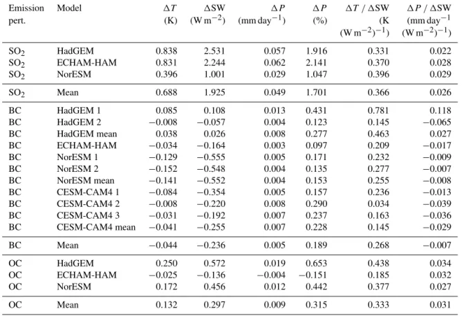
Table 2.Summary of global mean annual average climate responses.
Emission Model 1T 1SW 1P 1P 1T / 1SW 1P / 1SW pert. (K) (W m−2) (mm day−1) (%) (K (mm day−1 (W m−2)−1) (W m−2)−1)
SO2 HadGEM 0.838 2.531 0.057 1.916 0.331 0.022 SO2 ECHAM-HAM 0.831 2.244 0.062 2.141 0.370 0.028 SO2 NorESM 0.396 1.001 0.029 1.047 0.396 0.029
SO2 Mean 0.688 1.925 0.049 1.701 0.366 0.026
BC HadGEM 1 0.085 0.108 0.013 0.431 0.781 0.118 BC HadGEM 2 −0.008 −0.057 0.004 0.123 0.145 −0.065 BC HadGEM mean 0.038 0.026 0.008 0.277 0.463 0.027 BC ECHAM-HAM −0.034 −0.164 0.003 0.097 0.209 −0.017 BC NorESM 1 −0.129 −0.555 0.005 0.171 0.232 −0.009 BC NorESM 2 −0.152 −0.548 0.004 0.135 0.277 −0.007 BC NorESM mean −0.141 −0.552 0.004 0.153 0.255 −0.008 BC CESM-CAM4 1 −0.084 −0.354 0.005 0.157 0.236 −0.013 BC CESM-CAM4 2 −0.008 −0.220 0.008 0.290 0.034 −0.039 BC CESM-CAM4 3 −0.031 −0.192 0.007 0.237 0.163 −0.036 BC CESM-CAM4 mean −0.041 −0.255 0.007 0.228 0.145 −0.029
BC Mean −0.044 −0.236 0.005 0.189 0.268 −0.007
OC HadGEM 0.250 0.572 0.019 0.653 0.438 0.034 OC ECHAM-HAM −0.025 −0.136 −0.004 −0.151 0.185 0.032 OC NorESM 0.172 0.456 0.012 0.442 0.377 0.027
OC Mean 0.132 0.297 0.009 0.315 0.333 0.031
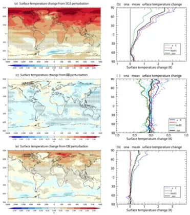
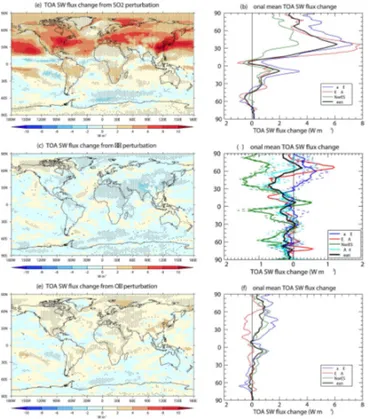
global mean surface temperature increases by 0.69 K. The zonal mean temperature change is positive at all latitudes and increases with increasing latitude, with a multi-model mean increase of around 2.5 K at the North Pole (Fig. 5b). Fig-ure 5a shows warming over almost all areas of the globe, including all land areas. As shown by the stippling, these temperature responses are significant throughout almost all the Northern Hemisphere, and much of the Southern Hemi-sphere. Most of the Northern Hemisphere land shows warm-ing of at least 1 K, with some northern regions exceedwarm-ing 2 K. These temperature responses can be understood further by comparison with the TOA SW flux changes. The global mean TOA SW flux change is positive for all three model sim-ulations (Fig. 4c). HadGEM, which has the strongest tem-perature response, also has the largest change in TOA SW flux, while NorESM, which has the weakest temperature re-sponse, has the smallest change in TOA SW flux. The ratio of temperature change to SW flux change is similar between the models (0.33–0.40 K (W m−2)−1, Table 2). The strongest increase in TOA SW flux change occurs in the Northern Hemisphere mid-latitudes, where the anthropogenic emis-sions are largest (Fig. 6b). There is good agreement be-tween the three models in the zonal distribution of TOA SW flux change, although NorESM shows smaller values in the Northern Hemisphere, which may explain the weaker tem-perature increase in this model compared to the others. The
multi-model mean changes are significant throughout most of the Northern Hemisphere (Fig. 6a). There are regions of strong TOA SW flux change over Europe, the eastern USA and China, which correspond to locations with the largest anthropogenic emissions. Over Europe and the eastern USA, this explains the relatively strong warming in these regions (Fig. 5a). The positive TOA SW flux change over China also extends in a band over the North Pacific. This is consistent with the decreased aerosol concentrations in this region due to the reduced emissions in China. As well as the direct radia-tive effects, the reduced aerosols would also cause changes in cloud cover. It was shown by Wang et al. (2014) that Chinese aerosol emissions increased cloud cover over the North Pa-cific, so removing these aerosols would reduce cloud cover. A similar region of positive TOA SW flux change also oc-curs over the North Atlantic, which is similarly due to weaker aerosol–radiation and aerosol–cloud effects over this region resulting from the aerosol emissions reductions over the east-ern USA. The regions of negative TOA SW flux change in the Pacific and Atlantic just north of the equator relate to a north-ward shift in the ITCZ, which increases the cloud cover north of the equator and decreases it to the south. This northward ITCZ shift is expected due to the hemispherically asymmet-ric warming (Rotstayn et al., 2000; Broccoli et al., 2006).
Figure 4.Summary of global mean annual average changes in(a, b)surface temperature,(c, d)all-sky TOA SW flux and(e, f) pre-cipitation. In the left panels the values shown for the BC simulations are the means for each model (where more than one simulation was run). The values for the individual BC simulations are shown in the right panels. The error bars indicate the 95 % confidence interval on the error in the mean (2σ/√n, wherenis the number of years of data included in the mean; i.e.nis 50×the number of ensemble members).
flux (Figs. 5a and 6a), the most pronounced being over the ocean north of Europe. These correspond to regions with large reductions in sea-ice (not shown). All three models agree on a large loss of Arctic sea-ice, due to the strong Northern Hemisphere warming. In the Southern Hemisphere, all three models actually show a region of increased sea-ice east of the Antarctic Peninsula, which explains the reduced temperatures and decreased TOA SW flux there.
The removal of anthropogenic SO2 emissions results in an increase in global mean precipitation (Fig. 4e). This in-crease is expected due to the inin-creased surface temperature. The multi-model mean percentage precipitation change per unit warming can be calculated from Table 2 as 2.50 % K−1, which is consistent with the value for SO4found by Andrews et al. (2010) (2.46±0.11 % K−1). While there is a global increase in precipitation, the Southern Hemisphere actually shows an overall decrease in precipitation (Fig. 7b). This is
Figure 5.Annual average change in surface temperature for (a, b)SO2,(c, d)BC and(e, f)OC perturbations. Left column: multi-model mean maps. Right column: zonal mean. In(a, c, e), stippling shows points where the response is significant at the 95% level (de-termined by a student’sttest using all years of all models).
Figure 6.Annual average change in all-sky TOA SW flux for(a, b)SO2,(c, d)BC and(e, f)OC perturbations. Left column: multi-model mean maps. Right column: zonal mean. In(a, c, e), stippling shows points where the response is significant at the 95 % level.
the northward ITCZ shift and corresponding changes in cir-culation.
Overall the models agree qualitatively on the climate re-sponse to removing anthropogenic SO2emissions, showing Northern Hemisphere warming and a northward shift in the ITCZ. HadGEM and ECHAM-HAM show very good quan-titative agreement in the response.
3.2 Response to perturbing black carbon emissions For the BC perturbation experiments, we consider, in addi-tion to the original simulaaddi-tions from HadGEM, ECHAM-HAM and NorESM, one extra ensemble member from each of HadGEM and NorESM, and three ensemble members from CESM-CAM4. For the calculations of multi-model means, we take the mean of the mean values for each model. The temperature response to removing anthropogenic BC emissions is much smaller overall than the response to per-turbing SO2emissions (Fig. 4 and Table 2). All the models except HadGEM show a net decrease in global mean sur-face temperature (Fig. 4a). This results in a small negative multi-model mean value for the global surface temperature response. However, we note the results of Myhre and Sam-set (2015) which indicate that climate models may underes-timate the forcing from BC by around 10 %. Figure 4b shows the temperature response in the individual model members.
Figure 7.Annual average change in precipitation for(a, b)SO2,(c, d)BC and(e, f)OC perturbations. Left column: multi-model mean maps. Right column: zonal mean. In(a, c, e), stippling shows points where the response is significant at the 95 % level.
This shows that HadGEM member 1 has a significant in-crease in global mean surface temperature, while the other simulations all show a decrease, although the sign of this re-sponse is uncertain in the cases of HadGEM member 2 and CESM-CAM4 member 2.
A similar pattern is seen for the change in TOA SW flux (Fig. 4c). For the majority of the simulations the ratio of temperature change to SW flux change is between 0.21 and 0.28 K (W m−2)−1 (Table 2) which is smaller than for SO2; however the HadGEM member 1 and CESM-CAM4 member 2 simulations are outliers with ratios of 0.78 and 0.03 K (W m−2)−1respectively.
The multi-model mean temperature response is within
±0.5 K everywhere (Fig. 5c). These temperature changes are significant in large parts of the Southern Hemisphere ocean and the tropical Pacific but less so in the Northern Hemi-sphere. The TOA SW flux change is also relatively small everywhere,with the strongest TOA SW flux decrease over northern India (Fig. 6c). However, the changes in TOA SW flux are significant over large areas of land in the Northern Hemisphere, in general over areas with high anthropogenic BC emissions.
in each model. This can be seen in Fig. 5d, which shows the range of zonal mean temperature responses between models. NorESM shows relatively strong cooling, which is stronger towards high latitudes, reaching around−0.4 K at the North Pole. In contrast, HadGEM shows warming in the North-ern Hemisphere, but to different degrees in the two ensem-ble members: in member 1 the temperature increases towards the North Pole, reaching 0.4 K; in contrast member 2 shows only slight warming, and a decrease in temperature at the pole. ECHAM-HAM shows a weak response in general but a small increase towards the North Pole. The three CESM-CAM4 members show different behaviour: all three show weak cooling at most latitudes, but north of around 60◦N
member 2 shows warming, which increases towards the pole and reaches 0.6 K. The zonal mean TOA SW flux change also shows large differences between models (Fig. 6d), which helps to explain the range of temperature responses in each model in the Northern Hemisphere.
The spatial responses in each of the model simulations can be seen in Figs. S2–S6, and can explain some of the differ-ences between models discussed above. HadGEM member 1 shows warming in the Arctic and over most of the Northern Hemisphere mid-latitudes, including Europe, which is unex-pected since anthropogenic BC emissions are relatively large there (Fig. S2a). This is due to increased TOA SW flux over Europe (Fig. S2c). Inspection of cloud and snow cover fields (not shown) shows that this is in fact a result of a combination of reduced cloud cover and reduced snow cover over northern Europe; these changes are likely due to circulation changes, and their combined effect is enough to more than balance the negative forcing from local removal of BC. The warming in the Arctic is linked to decreases in sea-ice (Fig. S2e) and collocated increases in TOA SW flux (Fig. S2c). HadGEM member 2 shows warming over much of Russia but cooling over North America (Fig. S2b). There is also strong warming along the south-eastern edge of Greenland and in the Barents Sea, which is linked to increased TOA SW flux (Fig. S2d) and large decreases in sea-ice (Fig. S2f). Both HadGEM members show strong decreases in TOA SW flux over India due to the emissions reductions, but these do not translate to strong temperature decreases. ECHAM-HAM also shows some localized warming in the Arctic, but cooling in much of the rest of the Northern Hemisphere (Fig. S3a), although most of this is not significant. As in HadGEM, the regions of Arctic warming are collocated with increased TOA SW flux (Fig. S3b) and decreased sea-ice (Fig. S3c). There are regions with decreased TOA SW flux over India, China and the eastern USA, which correspond to large reductions in BC emissions (Fig. S3b). In contrast, both NorESM mem-bers show cooling in the Arctic and significant cooling over much of the globe (Fig. S4a and b). In both members this cor-responds to decreased TOA SW flux over much of the Arctic and most of the northern hemispere land area (Fig. S4c and d). There are regions with increases in sea-ice, such as in the Barents Sea in Fig. S4f, but also small regions where the
sea-ice decreases, although these decreases are generally not sig-nificant (Fig. S4e and f). The three CESM-CAM4 members show different temperature responses in the Arctic: mem-ber 1 shows very little temperature response in the Arctic (Fig. S5a), while member 2 shows significant warming over much of the Arctic (Fig. S5b); member 3 shows cooling of a similar magnitude over the Arctic (Fig. S6a). Correspond-ing to the warmer Arctic temperatures in member 2, there are also widespread decreases in Arctic sea-ice (Fig. S5f), while member 1 shows more mixed sea-ice changes (Fig. S5e) and member 3 shows some regions with increase sea-ice (Fig. S6c). Member 1 shows significant cooling in much of the Southern Hemisphere ocean, while members 2 and 3 show only weak temperature responses. Both members show significant cooling in the North Pacific, linked to the reduc-tion in aerosol emissions from China. Compared to mem-bers 2 and 3, member 1 shows stronger decreases in TOA SW flux over China and Europe in response to the emissions reductions, which could explain the stronger overall temper-ature reduction in member 1 (Figs. S5c, d and 6b).
The global mean precipitation response to removing an-thropogenic BC emissions is relatively small (Fig. 4e and f). Despite the different signs of temperature response, the global precipitation increases in all the model simulations. This is not surprising since the removal of BC from the at-mosphere will lead to a negative atmospheric forcing, which in turn is expected to lead to increased precipitation (An-drews et al., 2010). NorESM shows a pronounced southward shift in the position of the ITCZ, which is consistent with the cooling in the Northern Hemisphere in these simulations (Fig. 7d). HadGEM member 1 shows a weak northward shift in the ITCZ, while the other model simulations do not show a coherent shift in its position. The opposing direction of the ITCZ shift in HadGEM member 1 and NorESM partly explains why the model-mean responses are generally rel-atively weak everywhere (Fig. 7c). It is interesting to note that over India, where the anthropogenic BC emissions are large, the removal of the BC emissions results in a decrease, rather than an increase, in precipitation. These precipitation changes are driven by circulation changes (e.g. the southward shift in the ITCZ) which dominate over the local effects on precipitation due to BC removal causing destabilization of the atmosphere.
3.3 Response to perturbing organic carbon emissions The multi-model mean response to removing anthropogenic OC emissions is an increase in global mean surface temper-ature (Fig. 4a and Table 2). HadGEM and NorESM show a clear increase in surface temperature, with the largest re-sponse in HadGEM; ECHAM-HAM shows a weak reduc-tion in global mean surface temperature, although the error bars indicate some uncertainty in the sign of this response. HadGEM and NorESM show an increase in the zonal mean surface temperature throughout the Northern Hemisphere, increasing towards the pole; ECHAM-HAM shows almost no change in the zonal mean surface temperature (Fig. 5f). Despite the different behaviour in ECHAM-HAM compared with the other models, there are broad areas in the Northern Hemisphere where the temperature changes are significant, including over much of Europe (Fig. 5e).
The TOA SW flux change is weakly positive over most of the Northern Hemisphere, and is mostly not significant (Fig. 6e). HadGEM and NorESM show an increase in zonal mean TOA SW flux over the Northern Hemisphere (Fig. 6f), and in particular show increased TOA SW flux over the mid-latitudes, which have the largest anthropogenic OC emis-sions (Fig. 1e). In contrast, ECHAM-HAM shows a decrease in TOA SW flux over the Northern Hemisphere mid-latitudes (Fig. 6f). Inspection of spatial maps (not shown) indicate that this is due to decreased SW flux over Europe and the east-ern USA, despite the reduced OC emissions in these regions. This may be due to natural variability in cloud cover over these regions driven by changes in atmospheric circulation patterns. The TOA SW flux change from the OC emissions perturbation seems to be much weaker in ECHAM-HAM than in the other models, so natural variability may domi-nate.
The global mean precipitation changes in each model are consistent with their respective temperature responses: HadGEM and NorESM show an increase in global precipi-tation, while ECHAM-HAM shows a decrease (Fig. 4e). De-spite the variation in temperature responses, all three models show a northward shift in the ITCZ (Fig. 7f). The changes in precipitation patterns are similar to those for the SO2 ex-periments but with weaker magnitude (compare Figs. 7c and e).
Overall the response to removal of anthropogenic OC emissions is an increase in surface temperature and precip-itation, primarily in the Northern Hemisphere. The spatial patterns of changes in these quantities are broadly similar to those for the SO2 emissions perturbation, but with smaller magnitude.
4 Discussion
The three models are in good agreement about the impacts of removing anthropogenic SO2 emissions, all showing a
warming concentrated in the Northern Hemisphere and a northward shift in the ITCZ, bringing more precipitation to the Northern Hemisphere. Further precipitation increases are seen in the Northern Hemisphere due to the increased tem-perature. NorESM gives a weaker overall response than the other two models. This is not surprising since NorESM has a lower SO4burden than the other models, so the SO2 emis-sions changes will have less impact. Furthermore, NorESM is known to have a relatively low climate sensitivity (An-drews et al., 2012), which Iversen et al. (2013) attribute to a strong Atlantic Meridional Overturning Circulation in NorESM. This may explain the smaller changes in Arctic sea-ice extent in NorESM than in the other two models in the SO2 experiment, reducing the impact of the additional positive feedback on temperature of the melting ice.
The response to removing anthropogenic OC emissions is similar to that for removing SO2 in terms of tempera-ture change per unit SW flux change (Table 2). The abso-lute magnitude of the response is about 5 times smaller for OC. ECHAM-HAM appears to have a weaker response to the removal of OC than the other models, and this is within the range of natural variability between individual years. The other models show similar patterns of response to those in the SO2experiment, but with weaker magnitude.
or other high albedo surfaces, so these effects will be much weaker in the control simulation in HadGEM and ECHAM than in the other models. Removal of anthropogenic BC emissions will therefore have a smaller impact in the mod-els with less high-level BC since the BC forcing in the con-trol simulation is weak to begin with. The climate responses in HadGEM may therefore be driven by changes in circula-tion, leading to, for example, the change in cloud and snow cover over Europe in HadGEM member 1. These circulation changes overwhelm the relatively weak forcing from the BC emissions perturbation. Apart from the HadGEM simulation the models suggest a lower ratio of temperature change to SW flux change for BC than for OC and SO2.
The results from this study show that there is large uncer-tainty as to the climate response to removing anthropogenic BC emissions. The different behaviour between models is due partly to the different atmospheric BC distributions in the models, as shown in Fig. 1. Accurately representing the cor-rect BC distribution in GCMs is very difficult (Samset et al., 2014). Recent studies (e.g. Schwarz et al., 2013; Hodnebrog et al., 2014; Samset et al., 2014) have compared BC distribu-tions in GCMs and CTMs with data from observational stud-ies such as the HIPPO campaign (Wofsy, 2011), which pro-vided observations from a large spatial area over the Pacific. They found that the models had too much BC at high alti-tudes in these regions, and that the BC lifetime was generally too long. Recent modifications to the convective scavenging scheme in HadGEM (which are included in the model set-up used here) were designed to reduce the amount of high-level BC to give better agreement with the HIPPO observations. The result of these changes is that HadGEM has less BC at high levels globally than the other models (except ECHAM-HAM), and a much shorter BC and OC lifetime (Table 1). ECHAM-HAM also has less BC at high levels, and a short BC lifetime. In contrast, NorESM and CESM-CAM4 have much more high-level BC and longer BC lifetimes, which may overestimate the direct forcing from anthropogenic BC (consistent with Samset et al., 2014) and may therefore exag-gerate the impact of removing anthropogenic BC emissions. The true BC distribution at high levels is most likely some-where in between these model estimates, while at lower lev-els the emissions are likely underestimated (Hodnebrog et al., 2014).
A further feature influencing the results in this study is the contribution of changes in sea-ice extent. Particularly for the OC and BC emissions perturbations, which give a weaker forcing than the SO2emissions perturbations, these sea-ice changes appear to be due to natural variability, rather than a forced response. However, they do contribute to the to-tal SW flux changes and surface temperature changes. This adds an extra element of natural variability that is not an issue in atmosphere-only simulations, which have fixed SSTs and prescribed sea-ice. This motivated our decision to perform three additional simulations, in order to increase our sample size. It can be seen from these simulations that the sea-ice
responds quite differently to the BC perturbation in different simulations, even in two simulations from the same model.
It is interesting to note the range of climate responses be-tween models, and even bebe-tween different simulations run by the same model. This highlights the importance of using an ensemble of simulations in studies such as this, where natural variability is a relatively large contributor, and differences in the formulation of individual models can have a large impact on the results. It is also interesting to note the very similar be-haviour of the two NorESM members compared to the quite different responses between the individual members in the other models. In all cases the different members were gen-erated by initializing with a different atmospheric state but keeping everything else the same. This further emphasizes the importance of using more than one model, since different models have different sensitivity to small perturbations in the initial conditions.
5 Conclusions
Air quality policies now and in the future will lead to reduced emissions of aerosols and other SLCPs. This study aims to evaluate the possible climate impacts of these emissions re-ductions, by considering a set of extreme idealized scenarios in which 100 % of the land-based anthropogenic emissions of individual aerosol precursor species (BC, OC and SO2) are removed. The experiments were performed mainly using three AOGCMs with interactive aerosols and chemistry, in order to capture the fast and slow responses to these emis-sions perturbations as well as the uncertainties in these re-sponses. We also included additional simulations from an-other AOGCM (without interactive aerosols) for the BC ex-periments.
The results show strong impacts on climate of removing SO2emissions, with an increase in global mean surface tem-perature, focussed mainly in the Northern Hemisphere, and a northward shift in the ITCZ, driving changes in precipi-tation patterns particularly in tropical regions. We note that the models used in this study do not represent nitrate chem-istry. This means that they may be overestimating the cli-mate responses to removal of SO2emissions, since reducing SO4would increase the potential amount of ammonium ni-trate aerosol formation, counteracting some of the effects of the reduced SO4aerosol (West et al., 1999; Bellouin et al., 2011).
experi-ments removes much of the variability that we see in fully-coupled AOGCMs due to responses in temperature and in ocean circulation, sea-ice, atmospheric circulation and cloud responses that are realized on long timescales. Overall the re-moval of OC emissions leads to similar patterns of response to the SO2experiments, but with much weaker magnitude. There is a weak northward shift in the ITCZ, and corre-sponding changes in precipitation. The BC response is more complex, and due to the large disagreement in response be-tween two of the models, we included five additional ensem-ble members. Even between two ensemensem-ble members from the same model there are large differences in the surface temper-ature and precipitation responses. From this study we con-clude that, while BC mitigation is unlikely to be detrimental to climate (like in the case of SO2and OC mitigation), the climate benefits are likely to be very small, and may not be discernable above natural variability in the climate.
The Supplement related to this article is available online at doi:10.5194/acp-15-8201-2015-supplement.
Author contributions. Model simulations were performed by L. H. Baker (HadGEM), D. J. L.Olivié (NorESM), R. Cherian (ECHAM-HAM) and Ø. Hodnebrog (CESM-CAM4). Analysis of the results was performed by L. H. Baker with contributions from D. J. L.Olivié. L. H. Baker prepared the manuscript with contribu-tions from all co-authors.
Acknowledgements. The research leading to these results has received funding from the European Union Seventh Framework Programme (FP7/2007-2013) under grant agreement no 282688 – ECLIPSE. The ECHAM-HAM model is developed by a consortium composed of ETH Zurich, Max Planck Institut für Meteorologie, Forschungszentrum Jülich, University of Oxford, the Finnish Meteorological Institute and the Leibniz Institute for Tropospheric Research, and managed by the Center for Climate Systems Modeling (C2SM) at ETH Zurich. R. Cherian and J. Quaas acknowledge the computing time provided by the German High Performance Computing Centre for Climate and Earth System Research (Deutsches Klimarechenzentrum, DKRZ). L. Baker and W. Collins acknowledge use of the MONSooN system, a collaborative facility supplied under the Joint Weather and Climate Research Programme, which is a strategic partnership between the Met Office and the Natural Environment Research Council. Ø. Hodnebrog and G. Myhre acknowledge additional funding from the Research Council of Norway through the SLAC project.
Edited by: F. Fierli
References
Abdul-Razzak, H. and Ghan, S. J.: A parameterization of aerosol activation: 2. Multiple aerosol types, J. Geophys. Res.-Atmos., 105, 6837–6844, 2000.
Abdul-Razzak, H. and Ghan, S. J.: A parameterization of aerosol activation 3. Sectional representation, J. Geophys. Res.-Atmos., 107, AAC1.1–AAC1.6, doi:10.1029/2001JD000483, 2002. Amann, M., Klimont, Z., and Wagner, F.: Regional and Global
Emissions of Air Pollutants: Recent Trends and Future Scenar-ios, Annu. Rev. Env. Resour., 38, 31–55, 2013.
Andrews, T., Forster, P. M., Boucher, O., Bellouin, N., and Jones, A.: Precipitation, radiative forcing and global temperature change, Geophys. Res. Lett., 37, L14701, doi:10.1029/2010GL043991, 2010.
Andrews, T., Gregory, J. M., Webb, M. J., and Taylor, K. E.: Forcing, feedbacks and climate sensitivity in CMIP5 coupled atmosphere-ocean climate models, Geophys. Res. Lett., 39, L09712, doi:10.1029/2012GL051607, 2012.
Ban-Weiss, G. A., Cao, L., Bala, G., and Caldeira, K.: Dependence of climate forcing and response on the altitude of black carbon aerosols, Clim. Dynam., 38, 897–911, 2012.
Bellouin, N., Rae, J., Jones, A., Johnson, C., Haywood, J., and Boucher, O.: Aerosol forcing in the Climate Model Intercom-parison Project (CMIP5) simulations by HadGEM2-ES and the role of ammonium nitrate, J. Geophys. Res., 116, D20206, doi:10.1029/2011JD016074, 2011.
Bellouin, N., Baker, L., Cherian, R., Hodnebrog, O., Olivié, D., Samset, B., MacIntosh, C., Esteve-Martinez, A., and Myhre, G.: Regional and seasonal radiative forcing by perturbations to aerosol and ozone precursor emissions, in preparation, 2015. Bentsen, M., Bethke, I., Debernard, J. B., Iversen, T., Kirkevåg,
A., Seland, Ø., Drange, H., Roelandt, C., Seierstad, I. A., Hoose, C., and Kristjánsson, J. E.: The Norwegian Earth Sys-tem Model, NorESM1-M – Part 1: Description and basic evalu-ation of the physical climate, Geosci. Model Dev., 6, 687–720, doi:10.5194/gmd-6-687-2013, 2013.
Bollasina, M. A., Ming, Y., and Ramaswamy, V.: Anthropogenic aerosols and the weakening of the South Asian summer mon-soon, Science, 334, 502–505, 2011.
Boucher, O., Randall, D., Artaxo, P., Bretherton, C., Feingold, G., Forster, P., Kerminen, V.-M., Kondo, Y., Liao, H., Lohmann, U., Rasch, P., Satheesh, S. K., Sherwood, S., Stevens, B., and Zhang, X.-Y.: Clouds and aerosols, in: Climate Change 2013: The Physical Science Basis, Contribution of working group I to the fifth assessment report of the intergovernmental panel on cli-mate change, 571–657, Cambridge University Press, Cambridge, UK and New York, NY, USA, 2013.
Broccoli, A., Dahl, K., and Stouffer, R.: Response of the ITCZ to Northern Hemisphere cooling, Geophys. Res. Lett., 33, L01702, doi:10.1029/2005GL024546, 2006.
Ceppi, P., Hwang, Y.-T., Liu, X., Frierson, D. M., and Hart-mann, D. L.: The relationship between the ITCZ and the South-ern Hemispheric eddy-driven jet, J. Geophys. Res.-Atmos., 118, 5136–5146, 2013.
Collins, W. D.: Parameterization of generalized cloud overlap for ra-diative calculations in general circulation models, J. Atmos. Sci., 58, 3224–3242, 2001.
po-tentials for near-term climate forcers, Atmos. Chem. Phys., 13, 2471–2485, doi:10.5194/acp-13-2471-2013, 2013.
Danabasoglu, G., Bates, S. C., Briegleb, B. P., Jayne, S. R., Jochum, M., Large, W. G., Peacock, S., and Yeager, S. G.: The CCSM4 ocean component, J. Climate, 25, 1361–1389, 2012. Eckhardt, S., Quennehen, B., Olivié, D. J. L., Berntsen, T. K.,
Cherian, R., Christensen, J. H., Collins, W., Crepinsek, S., Daskalakis, N., Flanner, M., Herber, A., Heyes, C., Hodnebrog, Ø., Huang, L., Kanakidou, M., Klimont, Z., Langner, J., Law, K. S., Massling, A., Myriokefalitakis, S., Nielsen, I. E., Nøjgaard, J. K., Quaas, J., Quinn, P. K., Raut, J.-C., Rumbold, S. T., Schulz, M., Skeie, R. B., Skov, H., Lund, M. T., Uttal, T., von Salzen, K., Mahmood, R., and Stohl, A.: Current model capabilities for simulating black carbon and sulfate concentrations in the Arc-tic atmosphere: a multi-model evaluation using a comprehensive measurement data set, Atmos. Chem. Phys. Discuss., 15, 10425– 10477, doi:10.5194/acpd-15-10425-2015, 2015.
Edwards, J. and Slingo, A.: Studies with a flexible new radiation code. I: Choosing a configuration for a large-scale model, Q. J. Roy. Meteor. Soc., 122, 689–719, 1996.
Emmons, L. K., Walters, S., Hess, P. G., Lamarque, J.-F., Pfister, G. G., Fillmore, D., Granier, C., Guenther, A., Kinnison, D., Laepple, T., Orlando, J., Tie, X., Tyndall, G., Wiedinmyer, C., Baughcum, S. L., and Kloster, S.: Description and evaluation of the Model for Ozone and Related chemical Tracers, version 4 (MOZART-4), Geosci. Model Dev., 3, 43–67, doi:10.5194/gmd-3-43-2010, 2010.
Feichter, J., Kjellström, E., Rodhe, H., Dentener, F., Lelieveldi, J., and Roelofs, G.-J.: Simulation of the tropospheric sulfur cycle in a global climate model, Atmos. Environ., 30, 1693–1707, 1996. Flanner, M. G.: Arctic climate sensitivity to local black carbon, J.
Geophys. Res.-Atmos., 118, 1840–1851, 2013.
Flanner, M. G., Zender, C. S., Randerson, J. T., and Rasch, P. J.: Present-day climate forcing and response from black car-bon in snow, J. Geophys. Res.-Atmos., 112, D11202, doi:10.1029/2006JD008003, 2007.
Gedney, N., Huntingford, C., Weedon, G., Bellouin, N., Boucher, O., and Cox, P.: Detection of solar dimming and brightening effects on Northern Hemisphere river flow, Nat. Geosci., 7, 796–800, 2014.
Gent, P. R., Danabasoglu, G., Donner, L. J., Holland, M. M., Hunke, E. C., Jayne, S. R., Lawrence, D. M., Neale, R. B., Rasch, P. J., Vertenstein, M., Worley, P. H., Yang, Z. L., and Zhang, M. H.: The community climate system model version 4, J. Climate, 24, 4973–4991, 2011.
Hewitt, H. T., Copsey, D., Culverwell, I. D., Harris, C. M., Hill, R. S. R., Keen, A. B., McLaren, A. J., and Hunke, E. C.: Design and implementation of the infrastructure of HadGEM3: the next-generation Met Office climate modelling system, Geosci. Model Dev., 4, 223–253, doi:10.5194/gmd-4-223-2011, 2011.
Hodnebrog, Ø., Myhre, G., and Samset, B. H.: How shorter black carbon lifetime alters its climate effect, Nat. Comm., 5, 5065, doi:10.1038/ncomms6065, 2014.
HTAP: Hemispheric Transport of Air Pollution 2010 – Part A: Ozone and Particulate Matter, Air Pollution Studies No. 17, edited by: Dentener, F., Keating, T., and Akimoto, H., United Nations, New York and Geneva, 2010.
Hunke, E. C. and Lipscomb, W. H.: CICE: the Los Alamos Sea Ice Model Documentation and Software User’s Manual Version 4.0 LA-CC-06-012, 2008.
Hwang, Y.-T., Frierson, D. M. W., and Kang, S. M.: Anthropogenic sulfate aerosol and the southward shift of tropical precipitation in the late 20th century, Geophys. Res. Lett., 40, 2845–2850, 2013. Inness, A., Baier, F., Benedetti, A., Bouarar, I., Chabrillat, S., Clark, H., Clerbaux, C., Coheur, P., Engelen, R. J., Errera, Q., Flem-ming, J., George, M., Granier, C., Hadji-Lazaro, J., Huijnen, V., Hurtmans, D., Jones, L., Kaiser, J. W., Kapsomenakis, J., Lefever, K., Leitão, J., Razinger, M., Richter, A., Schultz, M. G., Simmons, A. J., Suttie, M., Stein, O., Thépaut, J.-N., Thouret, V., Vrekoussis, M., Zerefos, C., and the MACC team: The MACC reanalysis: an 8 yr data set of atmospheric composition, Atmos. Chem. Phys., 13, 4073–4109, doi:10.5194/acp-13-4073-2013, 2013.
Iversen, T., Bentsen, M., Bethke, I., Debernard, J. B., Kirkevåg, A., Seland, Ø., Drange, H., Kristjansson, J. E., Medhaug, I., Sand, M., and Seierstad, I. A.: The Norwegian Earth System Model, NorESM1-M – Part 2: Climate response and scenario projec-tions, Geosci. Model Dev., 6, 389-415, doi:10.5194/gmd-6-389-2013, 2013.
Jungclaus, J., Fischer, N., Haak, H., Lohmann, K., Marotzke, J., Matei, D., Mikolajewicz, U., Notz, D., and Storch, J.: Character-istics of the ocean simulations in the Max Planck Institute Ocean Model (MPIOM) the ocean component of the MPI-Earth system model, Journal of Advances in Modeling Earth Systems, 5, 422– 446, 2013.
Kang, S. M., Held, I. M., Frierson, D. M., and Zhao, M.: The re-sponse of the ITCZ to extratropical thermal forcing: idealized slab-ocean experiments with a GCM, J. Climate, 21, 3521–3532, 2008.
Kirkevåg, A., Iversen, T., Seland, Ø., Hoose, C., Kristjánsson, J. E., Struthers, H., Ekman, A. M. L., Ghan, S., Griesfeller, J., Nils-son, E. D., and Schulz, M.: Aerosol–climate interactions in the Norwegian Earth System Model – NorESM1-M, Geosci. Model Dev., 6, 207–244, doi:10.5194/gmd-6-207-2013, 2013.
Klimont, Z., Smith, S. J., and Cofala, J.: The last decade of global anthropogenic sulfur dioxide: 2000–2011 emissions, Environ. Res. Lett., 8, 014003, doi:10.1088/1748-9326/8/1/014003, 2013. Klimont, Z., Kupiainen, K., Heyes, C., Purohit, P., Cofala, J., Rafaj, P., and Schoepp, W.: Global anthropogenic emissions of particulate matter, in preparation, 2015.
Koch, D. and Del Genio, A. D.: Black carbon semi-direct effects on cloud cover: review and synthesis, Atmos. Chem. Phys., 10, 7685–7696, doi:10.5194/acp-10-7685-2010, 2010.
Kristjánsson, J., Iversen, T., Kirkevåg, A., Seland, Ø., and De-bernard, J.: Response of the climate system to aerosol direct and indirect forcing: role of cloud feedbacks, J. Geophys. Res.-Atmos., 110, D24206, doi:10.1029/2005JD006299, 2005. Kvalevåg, M. M., Samset, B. H., and Myhre, G.: Hydrological
sen-sitivity to greenhouse gases and aerosols in a global climate model, Geophys. Res. Lett., 40, 1432–1438, 2013.
Lambert, F. H. and Webb, M. J.: Dependency of global mean precip-itation on surface temperature, Geophys. Res. Lett., 35, L16706, doi:10.1029/2008GL034838, 2008.
improvements and functional and structural advances in version 4 of the Community Land Model, Journal of Advances in Mod-eling Earth Systems, 3, M03001, doi:10.1029/2011MS00045, 2011.
Li, G. and Xie, S.-P.: Tropical Biases in CMIP5 Multimodel Ensem-ble: The Excessive Equatorial Pacific Cold Tongue and Double ITCZ Problems, J. Climate, 27, 1765–1780, 2014.
Lohmann, U., Stier, P., Hoose, C., Ferrachat, S., Kloster, S., Roeck-ner, E., and Zhang, J.: Cloud microphysics and aerosol indi-rect effects in the global climate model ECHAM5-HAM, At-mos. Chem. Phys., 7, 3425–3446, doi:10.5194/acp-7-3425-2007, 2007.
Mann, G. W., Carslaw, K. S., Spracklen, D. V., Ridley, D. A., Manktelow, P. T., Chipperfield, M. P., Pickering, S. J., and Johnson, C. E.: Description and evaluation of GLOMAP-mode: a modal global aerosol microphysics model for the UKCA composition-climate model, Geosci. Model Dev., 3, 519–551, doi:10.5194/gmd-3-519-2010, 2010.
Ming, Y. and Ramaswamy, V.: Nonlinear climate and hydrological responses to aerosol effects, J. Climate, 22, 1329–1339, 2009. Ming, Y., Ramaswamy, V., and Persad, G.: Two opposing effects of
absorbing aerosols on global-mean precipitation, Geophys. Res. Lett., 37, L13701, doi:10.1029/2010GL042895, 2010.
Myhre, G. and Samset, B. H.: Standard climate models radia-tion codes underestimate black carbon radiative forcing, Atmos. Chem. Phys., 15, 2883–2888, doi:10.5194/acp-15-2883-2015, 2015.
Myhre, G., Berglen, T. F., Johnsrud, M., Hoyle, C. R., Berntsen, T. K., Christopher, S. A., Fahey, D. W., Isaksen, I. S. A., Jones, T. A., Kahn, R. A., Loeb, N., Quinn, P., Remer, L., Schwarz, J. P., and Yttri, K. E.: Modelled radiative forcing of the direct aerosol effect with multi-observation evaluation, Atmos. Chem. Phys., 9, 1365–1392, doi:10.5194/acp-9-1365-2009, 2009.
Neale, R., Richter, J., Conley, A., Park, S., Lauritzen, P., Get-telm, A., Williamson, D., Rasch, P., Vavrus, S., Taylor, M., Collins, W., Zhang, M., and Lin, S.-J.: Description of the NCAR Community Atmosphere Model (CAM 4.0), Tech. rep., National Center for Atmospheric Research (NCAR), Boulder, Colorado, 2011.
Neale, R. B., Richter, J., Park, S., Lauritzen, P. H., Vavrus, S. J., Rasch, P. J., and Zhang, M.: The mean climate of the Community Atmosphere Model (CAM4) in forced SST and fully coupled ex-periments, J. Climate, 26, 5150–5168, 2013.
O’Connor, F. M., Johnson, C. E., Morgenstern, O., Abraham, N. L., Braesicke, P., Dalvi, M., Folberth, G. A., Sanderson, M. G., Telford, P. J., Voulgarakis, A., Young, P. J., Zeng, G., Collins, W. J., and Pyle, J. A.: Evaluation of the new UKCA climate-composition model – Part 2: The Troposphere, Geosci. Model Dev., 7, 41–91, doi:10.5194/gmd-7-41-2014, 2014.
Olivié, D., Peters, G., and Saint-Martin, D.: Atmosphere response time scales estimated from AOGCM experiments, J. Climate, 25, 7956–7972, 2012.
Osborne, J. M. and Lambert, F. H.: The missing aerosol response in twentieth-century mid-latitude precipitation observations, Nature Climate Change, 4, 374–379, 2014.
Pausata, F. S. R., Gaetani, M., Messori, G., Kloster, S., and Den-tener, F. J.: The role of aerosol in altering North Atlantic at-mospheric circulation in winter and its impact on air quality,
Atmos. Chem. Phys., 15, 1725–1743, doi:10.5194/acp-15-1725-2015, 2015.
Polson, D., Bollasina, M., Hegerl, G., and Wilcox, L.: Decreased monsoon precipitation in the northern hemisphere due to an-thropogenic aerosols, Geophys. Res. Lett., 41, 6023–6029, doi:10.1002/2014GL060811, 2014.
Quennehen, B., Raut, J.-C., Law, K. S., Ancellet, G., Clerbaux, C., Kim, S.-W., Lund, M. T., Myhre, G., Olivié, D. J. L., Safieddine, S., Skeie, R. B., Thomas, J. L., Tsyro, S., Bazureau, A., Bellouin, N., Daskalakis, N., Hu, M., Kanakidou, M., Klimont, Z., Kupi-ainen, K., Myriokefalitakis, S., Quaas, J., Rumbold, S. T., Schulz, M., Cherian, R., Shimizu, A., Wang, J., Yoon, S.-C., and Zhu, T.: Multi-model evaluation of short-lived pollutant distributions over East Asia during summer 2008, Atmos. Chem. Phys. Discuss., 15, 11049–11109, doi:10.5194/acpd-15-11049-2015, 2015. Ramanathan, V. and Carmichael, G.: Global and regional climate
changes due to black carbon, Nat. Geosci., 1, 221–227, 2008. Rosenfeld, D., Lohmann, U., Raga, G. B., O’Dowd, C. D.,
Kul-mala, M., Fuzzi, S., Reissell, A., and Andreae, M. O.: Flood or drought: how do aerosols affect precipitation?, Science, 321, 1309–1313, 2008.
Rotstayn, L. D. and Lohmann, U.: Tropical Rainfall Trends and the Indirect Aerosol Effect, J. Climate, 15, 2103–2116, 2002. Rotstayn, L. D., Ryan, B. F., and Penner, J. E.: Precipitation changes
in a GCM resulting from the indirect effects of anthropogenic aerosols, Geophys. Res. Lett., 27, 3045–3048, 2000.
Samset, B. H., Myhre, G., Herber, A., Kondo, Y., Li, S.-M., Moteki, N., Koike, M., Oshima, N., Schwarz, J. P., Balkanski, Y., Bauer, S. E., Bellouin, N., Berntsen, T. K., Bian, H., Chin, M., Diehl, T., Easter, R. C., Ghan, S. J., Iversen, T., Kirkevåg, A., Lamar-que, J.-F., Lin, G., Liu, X., Penner, J. E., Schulz, M., Seland, Ø., Skeie, R. B., Stier, P., Takemura, T., Tsigaridis, K., and Zhang, K.: Modelled black carbon radiative forcing and atmospheric lifetime in AeroCom Phase II constrained by aircraft observa-tions, Atmos. Chem. Phys., 14, 12465–12477, doi:10.5194/acp-14-12465-2014, 2014.
Sand, M., Berntsen, T. K., Kay, J. E., Lamarque, J. F., Seland, Ø., and Kirkevåg, A.: The Arctic response to remote and lo-cal forcing of black carbon, Atmos. Chem. Phys., 13, 211–224, doi:10.5194/acp-13-211-2013, 2013a.
Sand, M., Berntsen, T. K., Seland, Ø., and Kristjánsson, J. E.: Arctic surface temperature change to emissions of black carbon within Arctic or midlatitudes, J. Geophys. Res.-Atmos., 118, 7788– 7798, 2013b.
Schwarz, J. P., Samset, B. H., Perring, A. E., Spackman, J. R., Gao, R. S., Stier, P., Schulz, M., Moore, F. L., Ray, E. A., and Fa-hey, D. W.: Global-scale seasonally resolved black carbon verti-cal profiles over the Pacific, Geophys. Res. Lett., 40, 5542–5547, 2013.
Shindell, D. and Faluvegi, G.: Climate response to regional radiative forcing during the twentieth century, Nat. Geosci., 2, 294–300, 2009.
Shindell, D. T.: Inhomogeneous forcing and transient cli-mate sensitivity, Nature Climate Change, 4, 274–277, doi:10.1038/nclimate2136, 2014.
Smith, R., Jones, P., Briegleb, B., Bryan, F., Danabasoglu, G., Den-nis, J., Dukowicz, J., Eden, C., Fox-Kemper, B., Gent, P., Hecht, M., Jayne, S., Jochum, M., Large, W., Lindsay, K., Maltrud, M., Norton, N., Peacock, S., Vertenstein, M., and Yeager, S.: The Par-allel Ocean Program (POP) reference manual: Ocean component of the Community Climate System Model (CCSM), Los Alamos National Laboratory, LAUR-10-01853, 2010.
Søvde, O. A., Gauss, M., Smyshlyaev, S. P., and Isaksen, I. S.: Eval-uation of the chemical transport model Oslo CTM2 with focus on arctic winter ozone depletion, J. Geophys. Res.-Atmos., 113, D09304, doi:10.1029/2007JD009240, 2008.
Stevens, B., Giorgetta, M., Esch, M., Mauritsen, T., Crueger, T., Rast, S., Salzmann, M., Schmidt, H., Bader, J., Block, K., Brokopf, R., Fast, I., Kinne, S., Kornblueh, L., Lohmann, U., Pincus, R., Reichler, T., and Roeckner, E.: Atmospheric compo-nent of the MPI-M Earth System Model: ECHAM6, Journal of Advances in Modeling Earth Systems, 5, 146–172, 2013. Stier, P., Feichter, J., Kinne, S., Kloster, S., Vignati, E., Wilson, J.,
Ganzeveld, L., Tegen, I., Werner, M., Balkanski, Y., Schulz, M., Boucher, O., Minikin, A., and Petzold, A.: The aerosol-climate model ECHAM5-HAM, Atmos. Chem. Phys., 5, 1125–1156, doi:10.5194/acp-5-1125-2005, 2005.
Stohl, A., Aamaas, B., Amann, M., Baker, L. H., Bellouin, N., Berntsen, T. K., Boucher, O., Cherian, R., Collins, W., Daskalakis, N., Dusinska, M., Eckhardt, S., Fuglestvedt, J. S., Harju, M., Heyes, C., Hodnebrog, Ø., Hao, J., Im, U., Kanakidou, M., Klimont, Z., Kupiainen, K., Law, K. S., Lund, M. T., Maas, R., MacIntosh, C. R., Myhre, G., Myriokefalitakis, S., Olivié, D., Quaas, J., Quennehen, B., Raut, J.-C., Rumbold, S. T., Samset, B. H., Schulz, M., Seland, Ø., Shine, K. P., Skeie, R. B., Wang, S., Yttri, K. E., and Zhu, T.: Evaluating the climate and air quality impacts of short-lived pollutants, Atmos. Chem. Phys. Discuss., 15, 15155–15241, doi:10.5194/acpd-15-15155-2015, 2015. Tai, A., Martin, M., and Heald, C.: Threat to future global food
secu-rity from climate change and ozone air pollution, Nature Climate Change, 4, 817–821, 2014.
Textor, C., Schulz, M., Guibert, S., Kinne, S., Balkanski, Y., Bauer, S., Berntsen, T., Berglen, T., Boucher, O., Chin, M., Dentener, F., Diehl, T., Feichter, J., Fillmore, D., Ginoux, P., Gong, S., Grini, A., Hendricks, J., Horowitz, L., Huang, P., Isaksen, I. S. A., Iversen, T., Kloster, S., Koch, D., Kirkevåg, A., Kristjans-son, J. E., Krol, M., Lauer, A., Lamarque, J. F., Liu, X., Mon-tanaro, V., Myhre, G., Penner, J. E., Pitari, G., Reddy, M. S., Seland, Ø., Stier, P., Takemura, T., and Tie, X.: The effect of harmonized emissions on aerosol properties in global models – an AeroCom experiment, Atmos. Chem. Phys., 7, 4489–4501, doi:10.5194/acp-7-4489-2007, 2007.
Tsigaridis, K., Daskalakis, N., Kanakidou, M., Adams, P. J., Ar-taxo, P., Bahadur, R., Balkanski, Y., Bauer, S. E., Bellouin, N., Benedetti, A., Bergman, T., Berntsen, T. K., Beukes, J. P., Bian, H., Carslaw, K. S., Chin, M., Curci, G., Diehl, T., Easter, R. C., Ghan, S. J., Gong, S. L., Hodzic, A., Hoyle, C. R., Iversen, T., Jathar, S., Jimenez, J. L., Kaiser, J. W., Kirkevåg, A., Koch, D., Kokkola, H., Lee, Y. H, Lin, G., Liu, X., Luo, G., Ma, X., Mann, G. W., Mihalopoulos, N., Morcrette, J.-J., Müller, J.-F., Myhre, G., Myriokefalitakis, S., Ng, N. L., O’Donnell, D., Pen-ner, J. E., Pozzoli, L., Pringle, K. J., Russell, L. M., Schulz, M., Sciare, J., Seland, Ø., Shindell, D. T., Sillman, S., Skeie, R. B., Spracklen, D., Stavrakou, T., Steenrod, S. D., Takemura, T., Ti-itta, P., Tilmes, S., Tost, H., van Noije, T., van Zyl, P. G., von Salzen, K., Yu, F., Wang, Z., Wang, Z., Zaveri, R. A., Zhang, H., Zhang, K., Zhang, Q., and Zhang, X.: The AeroCom eval-uation and intercomparison of organic aerosol in global mod-els, Atmos. Chem. Phys., 14, 10845–10895, doi:10.5194/acp-14-10845-2014, 2014.
Vignati, E., Wilson, J., and Stier, P.: M7: an efficient size-resolved aerosol microphysics module for large-scale aerosol transport models, J. Geophys. Res.-Atmos., 109, D22202, doi:10.1029/2003JD004485, 2004.
Wang, Y., Wang, M., Zhang, R., Ghan, S. J., Lin, Y., Hu, J., Pan, B., Levy, M., Jiang, J. H., and Molina, M. J.: Assessing the effects of anthropogenic aerosols on Pacific storm track using a multiscale global climate model, P. Natl. Acad. Sci. USA, 111, 6894–6899, 2014.
West, J. J., Ansari, A. S., and Pandis, S. N.: Marginal PM2.5: Non-linear aerosol mass response to sulfate reductions in the east-ern United States, J. Air Waste Manage. Assoc., 49, 1415–1424, 1999.
Wofsy, S.: HIAPER Pole-to-Pole Observations (HIPPO): fine-grained, global-scale measurements of climatically important at-mospheric gases and aerosols, Philos. T. R. Soc. A, 369, 2073– 2086, 2011.