A conditional likelihood ratio test for structural models

(1)

A Conditional Likelihood Ratio Test for

Structural Models

Marcelo J. Moreira

∗

January 9, 2002

Abstract

This paper develops a general method for constructing similar tests based on the conditional distribution of nonpivotal statistics in a si-multaneous equations model with normal errors and known reduced-form covariance matrix. The test based on the likelihood ratio statistic is particularly simple and has good power properties. When identifi-cation is strong, the power curve of this conditional likelihood ratio test is essentially equal to the power envelope for similar tests. Monte Carlo simulations also suggest that this test dominates the Anderson-Rubin test and the score test. Dropping the restrictive assumption of disturbances normally distributed with known covariance matrix, approximate conditional tests are found that behave well in small sam-ples even when identification is weak.

JEL Classification: C12, C31.

Keywords: instrumental variables, similar tests, Wald test, likelihood ratio test, power envelope, confidence regions, 2SLS estimator, LIML estimator.

∗_°_c _{2001 Copyright. Lengthy discussions with Thomas Rothenberg were extremely}

(2)

1 Introduction

When making inferences about coefficients of endogenous variables in a struc-tural equation, applied researchers often rely on asymptotic approximations. However, as emphasized in recent work by Bound, Jaeger and Baker (1995) and Staiger and Stock (1997), these approximations are not satisfactory when instruments are weakly correlated with the regressors. In particular, if iden-tification can be arbitrarily weak, Dufour (1997) showed that Wald-type con-fidence intervals cannot have correct coverage probability while Wang and Zivot (1998) showed that the standard likelihood ratio test employing chi-square critical values do not have correct size. The problem arises because inference is based on nonpivotal statistics whose exact distributions depart substantially from their asymptotic approximations when identification is weak.

This paper develops a general procedure for constructing valid tests of structural coefficients based on the conditional distribution of nonpivotal statistics. When the reduced-form errors are normally distributed with a known covariance matrix, this procedure yields tests that are exactly similar; that is, their null rejection probabilities do not depend on the values of the unknown nuisance parameters. Simple modifications of these tests are shown to be approximately similar even when the errors are nonnormal and the reduced-form covariance matrix is unknown.

(3)

estimators, respectively, that have correct coverage probability even when instruments are weak and that are informative when instruments are good.

This paper is organized as follows. In Section 2, exact results are de-veloped for the special case of a two-equation model under the assumption that the reduced-form disturbances are normally distributed with known co-variance matrix. Sections 3 and 4 extend the results to more realistic cases, although at the cost of introducing some asymptotic approximations. Monte Carlo simulations suggest that these approximations are quite accurate. Sec-tion 5 compares the confidence region based on the condiSec-tional likelihood ratio test with the confidence region based on a score test that is also ap-proximately similar. Section 6 contains concluding remarks. All proofs are given in the appendix.

2 Known Covariance Matrix

2.1 The Model

To simplify exposition, consider a simple model in which the structural equa-tion of interest is

(1) y1 =y2β+u

where y1 and y2 are n × 1 vectors of observations on two endogenous

vari-ables, u is an n _× 1 unobserved disturbance vector, and β is an unknown scalar parameter. This equation is assumed to be part of a larger linear si-multaneous equations model which implies thaty2 is correlated withu. The

complete system contains exogenous variables which can be used as instru-ments for conducting inference on β. Specifically, it is assumed that the reduced form for Y = [y1, y2] can be written as

y1 = Zπβ+v1

(2)

y2 = Zπ+v2

where Z is an n _× k matrix of exogenous variables having full column rank

(4)

errors V = [v1, v2] are i.i.d. normally distributed with mean zero and 2 ×

2 nonsingular covariance matrix Ω = [ωi,j]. It is assumed that k > 1 so

the structural equation is “overidentified.” The goal here is to test the null hypothesis H0 :β =β0 against the alternativeH1 :β 6=β0.

Commonly used tests reject the null hypothesis when a test statistic _T takes on a value greater than a specified critical value c. The test is said to have size α if, when the null hypothesis is true,

Prob(_T > c)_≤α

for all admissible values of the nuisance parameters π and Ω. Since π and Ω are unknown, finding a test with correct size is nontrivial. Of course, if the null distribution of _T does not depend on the nuisance parameters, the 1₋α quantile of_T can be used for cand the null rejection probability will be identically equal toα. In that case, _T is said to be pivotal and the test is said to be similar.

Although structural coefficient tests based on pivotal statistics have been proposed in the literature (see, for example, Anderson and Rubin (1949), Kleibergen (2000), and Moreira (2001)), they sometimes have poor power properties. On the other hand, the Wald and likelihood ratio statistics most commonly employed in practice are not pivotal. However, under regularity conditions, these test statistics are asymptotically chi-square with one degree of freedom and tests using the 1₋α chi-square quantile for care asymptot-ically similar with size α. Unfortunately, ifπ cannot be bounded away from zero, their actual size can differ substantially from α since the asymptotic approximation will be very poor when the instruments are weakly correlated with y2.

(5)

statistics that are not boundedly pivotal. Here we will develop an alternative method to construct similar tests based on nonpivotal statistics under the assumption Ω is known.

2.2 Similar Tests Based on Nonpivotal Statistics

When Ω is known and the errors are normal, the probability model is a mem-ber of the curved exponential family and thek_×2 matrix Z′_Y _{is a sufficient}

statistic for the unknown parameters (β, π). Hence, any test depends on the data only through Z′_Y. _{However, for any known nonsingular, nonrandom}

2_×2 matrixD,the k_×2 matrixZ′_{Y D}_{is also sufficient. A convenient choice}

is the matrix D= [b,Ω−1

a], where b = (1,₋β0)′ and a = (β0,1)′. Then the

sufficient statistic can be represented by the pair of k_×1 vectors

S =Z′_{Y b}₌_Z′₍_y

1−y2β0) and T =Z′YΩ− 1

a.

The vectorSis normally distributed with meanZ′_Zπ₍_β₋_β

0) and covariance

matrix (b′_Ω_b₎_Z′_Z_;_T _{is independent of}_S_{and normally distributed with mean}

(a′_Ω−1

a)Z′_Zπ _{and covariance matrix (}_a′_Ω−1

a)Z′_Z_{, where} _a _{= (}_β,₁₎_. _Thus

we have partitioned the sufficient statistic into two independent, normally distributed vectors,T having a null distribution depending onπandShaving a null distribution not depending on π.

Any test statistic that depends only onS will be pivotal and can be used to form a similar test. Likewise, as discussed in Moreira (2001), similar tests can be constructed from pivotal statistics of the formg(T)′_S/p_g₍_T₎′_Z_′_Zg₍_T₎

whereg is any (measurable) k-dimensional vector depending on T. The goal here instead is to find a similar test at level α based on a nonpivotal test statistic ψ(S, T, β0). The following approach is suggested by the analysis

in Lehmann (1986, Chapter 4). Although the marginal distribution of ψ

(6)

Proposition 1: Suppose that ψ(S, t, β0) is a continuous random

vari-able under H0 for every t. Define c(t, β0, α) to be the 1−α quantile of the

null distribution of ψ(S, t, β0). Then the test that rejectsH0 if ψ(S, T, β0)>

c(T, β0, α) is similar at level α∈(0,1).

Moreira (2001) shows thatT =a′_Ω−1

a_·Z′_Z_b_π_{, where} _b_π _{is the maximum}

likelihood estimator of π when β is constrained to take the null value β0

and Ω is known. Therefore, this method of finding similar tests can be interpreted as adjusting the critical value based on a preliminary estimate of

π. Alternatively, this approach may be thought of as replacing the nonpivotal statistic ψ(S, T, β0) by the statistic ψ(S, T, β0)− c(T, β0, α) which yields a

test of correct size no matter what the value of π.

Although Proposition 1 can be applied to any continuously distributed test statistic depending on S and T, the details will be worked out here only for two special cases: the Wald test statistic based on the two-stage least squares estimator and the likelihood ratio test statistic.

2.2.1 A Conditional Wald Test

Let NZ = Z(Z′Z)−1Z′. Consider the Wald statistic centered around the

2SLS estimator:

(3) W0 =

(b2_SLS−β0) 2

y′

2NZy2

ˆ

σ2

where b2_SLS = (y2′NZy2)− 1

y′

2NZy1 and ˆσ 2

= [1₋b2_SLS]Ω[1−b2_SLS]′. Here,

the nonstandard structural error variance estimate exploits the fact that Ω is known. Since W0 depends on the data only through Z′Y, it can be

written as a function ofS, T and β0. Although in principle the critical value

function cW(t, β0, α) can be derived from the known distribution of S, a

simple analytical expression seems out of reach. A Monte Carlo simulation from the null distribution ofSis much simpler. Indeed, the applied researcher need only do a simulation for the actual value of T observed in the sample and for the particular β0 being tested; there is no need to derive the whole

(7)

Although a simple algebraic expression for the critical value function

cW(t, β0, α) is not available,some of its properties are known. For any

posi-tive integerr, letqα(r) denote the 1−αquantile of a chi-square distribution

with r degrees of freedom. Let ρ0 be the correlation coefficient between an

element of y1−y2β0 and the corresponding element of y2. Then,

Proposition 2: The critical value function for the conditional W0 test

satisfies

cW(t, β0, α) → q_α(1) as t′t→ ∞

cW(t, β0, α) → q_α(k)

ρ2 0

1₋ρ2 0

as t′_t _→₀

Note thatT is normal with a mean that is proportional toπ. When π is far from the origin, T′_T _{will take on large values with very high probability;}

the relevant critical value forW0is then the standard chi-square-one quantile.

When π is near the origin,T′_T _{is likely to be small and the relevant critical}

value for W0 may be very large ifρ 2

0 is near one.

2.2.2 The Conditional Likelihood Ratio Test

When Ω is known, the likelihood ratio statistic, defined to be two times the log of the likelihood ratio, is given by:

(4) LR0 = ¯λ

max

− a

′_Ω−1

Y′_{N Y}_Ω−1

a a′_Ω−1

a

where ¯λmax

is the largest eigenvalue of Ω−1_/2

Y′_{N Y}_Ω−1_/2

. This statistic can be written as a function of the sufficient statistics S and T. However, the expression is somewhat simpler when written in terms of the standardized statistics

¯

S= (Z′Z)

−1_/2

S

√

b′_Ω_b and

¯

T = (Z′Z)

−1_/2

T

√

a′_Ω−1_a

having covariance matrices equal to the identity matrix. Under the null hypothesis, ¯Shas mean zero so ¯S′_S¯_{is distributed as chi square with}_k_degrees

(8)

noncentrality proportional to π′_Z′_Zπ_{; it can be viewed as a natural statistic}

for testing the hypothesis that π= 0 under the assumption that β =β0.

In Appendix B, the following expression for the likelihood ratio statistic is derived:

(5) LR0 =

1 2

·

¯

S′_S¯₋_T¯′_T¯₊

q

[ ¯SS¯+ ¯T′_T¯_]2

−4[ ¯S′_S¯_·_T¯′_T¯₋_{( ¯}_S′_T¯₎2

]

¸

Whenk = 1,S¯and ¯T are scalars and theLR0 statistic collapses to the pivotal

statistic ¯S′_S.¯ _{In the overidentified case the}_LR

0statistic depends also on ¯T′T¯

and is no longer pivotal. Nevertheless, a similar test can be found by applying Proposition 1. Again, an analytic expression for the critical value function for the conditionalLR0 statistic is not available but the needed values can be

computed by simulation. Some general properties of the function are known.

Proposition 3: The critical value function for the conditional LR0 test

depends only on α, k, and ¯t′_t.¯ _{It satisfies}

cLR(¯t′t, k, α¯ ) → qα(1) as ¯t′¯t→ ∞

cLR(¯t′t, k, α¯ ) → qα(k) as ¯t′¯t→0

Table 1 presents the critical value function calculated from 10,000 Monte Carlo replications for the significance level of 5%. When k = 1, the true critical value function is a constant equal to 3.84 at level 5%. The slight variation in the first column of Table 1 is due to simulation error. For each

k, the critical value function has approximately an exponential shape, de-creasing from qα(k) at ¯t′t¯= 0 to qα(1) as ¯t′¯t tends to infinity. For example,

whenk = 4, the approximation c(¯t′_t,¯₄_,₀_._{05) = 3}_._{84 + 5}_._{65 exp(}₋¯_t′¯_t/_{7) seems}

to fit reasonably well.

(9)

hypothesis π= 0.The conditional approach has the advantage that it is not ad hocand the final test has correct size without unnecessarily wasting power. Figure 1 illustrates each method, sketching its respective critical values1

for different values of ¯t′_t¯_{when the number of instruments equals four.}

2.3 Monte Carlo Simulations

To evaluate the power of the conditional W0 and LR0 tests, a 1,000

repli-cation experiment was performed based on design I of Staiger and Stock (1997). The hypothesized value β0 is zero. The elements of the 100 ×4

matrix Z are drawn as independent standard normal and then held fixed over the replications. Two different values of the π vector are used so that the “population” first-stage F-statistic (in the notation of Staiger and Stock)

λ′_λ/k₌_π′_Z′_Zπ/₍_ω₂₂_k_{) takes the values 1 (weak instruments) and 10 (good}

instruments). The rows of (u, v2) are i.i.d. normal random vectors with unit

variances and correlation ρ. Results are reported for ρ taking the values 0.00, 0.50 and 0.99. The critical values for the conditional likelihood ratio and Wald tests were based on 1,000 replications.

In addition to the two conditional tests, denoted as LR∗

0 and W0∗, two

other similar tests were evaluated: the Anderson-Rubin test based on the statistic AR0 = ¯S′S¯ (modified to take into account that Ω is known) and

the score test based on the statistic LM0 =

¡_¯

T′_S¯¢2_/_T¯_{T .}¯ _{The latter test}

is described in Kleibergen (2000) and Moreira (2001). Figures 2-3 graph, for a fixed value of π and ρ, the rejection probabilities of the AR0, LM0,

conditional LR0 and conditional W0 tests as functions of the true value β. 2

The power envelope for similar tests is also included. In each figure, all four power curves are at approximately the 5% level when β equals β0. This

reflects the fact that each test is similar. As expected, the power curves become steeper as the quality of instruments improve.

1

The pre-testing procedure proposed by Zivot, Nelson and Startz (1998) is based on

theOLS estimator forπ. Instead, figure 1 sketches the critical value function based on a

pre-testing on the constrained maximum likelihood estimator for π.

2

As β varies, ω11 and ω12 change to keep the structural error variance and the

(10)

As expected, theAR0test has power considerably lower than the envelope

power. The LM0 test has relative low power either for the weak-instrument

case or for some alternatives β for the good-instrument case. Figures 2-3 also suggest that the conditional W0 test has poor power for some parts of

the parameter space. These poor power properties are not shared by the conditionalLR0 test. The conditional likelihood ratio test not only seems to

dominate the Anderson-Rubin test and the score test, but it also has power essentially equal to the power envelope for similar tests3

when identification is strong.

The good performance of the conditionalLR0 test is not surprising.

Var-ious authors have noticed that, in curved exponential models, the likelihood ratio test performs well for a wide range of alternatives. Van Garderen (2000) addresses this issue in the case the nuisance parameter is present only under the alternative.

3 Unknown Covariance Matrix

In practice, of course, the reduced-form covariance matrix Ω is not known and must be treated as an additional nuisance parameter. Under normality, the probability model remains curved exponential, but the sufficient statis-tic expands to (Z′_{Y, Y}′_Y₎_. _{However, the conditional approach developed in}

Section 2 cannot be easily applied in this context. Nevertheless, it seem plau-sible that the conditional tests can still be used after replacing the unknown Ω by some estimate since Ω can be well estimated regardless of the quality of the instruments. Furthermore, although motivated by the normal model, under relatively weak regularity conditions, the test statistics have limiting distributions that do not depend on the error distribution. Thus, modified versions of the tests developed under the restrictive assumptions of normal errors with known reduced form covariance matrix can be expected to behave

3

Other tests that have been proposed in the literature such as the Wald test based on

the LIML estimator and the GM M0 test proposed by Wang and Zivot (1998) were also

(11)

well under much weaker assumptions.

3.1 A Conditional Wald Test

The OLS estimator of Ω is given by Ω =b Y′_M

ZY /(n − k) where MZ =

I₋Z(Z′_Z₎−1

Z′_{. It is natural then to consider the test statistic}

(6) W = (b2SLS −β0)

2

y′

2NZy2

˜

σ2

where ˜σ2

= [1₋b2_SLS]Ω[1b −b2_SLS]′. The critical value function derived for

W0 can then be applied here, but with Te=Z′YΩb− 1

a instead ofT. That is, when Ω is unknown, one would reject the null hypothesis that β =β0 if

W ₋cW(T , βe 0, α)>0.

3.2 The Likelihood Ratio Test

Likewise, the LR0 test statistic also depends on Ω and, therefore, cannot

be used when the covariance matrix of the reduced form disturbances is unknown. Again, a natural modification is to replace Ω by its OLS estimator:

LR1 =λ max

− a′Ωˆ−

1

Y′_N

ZYΩˆ−1a

a′_Ωˆ−1_a

whereλmax

is the largest eigenvalue ofΩb−1_/2

Y′_N

ZYΩb−1/2. Alternatively, one

could use the likelihood ratio statistic for the case Ω is unknown:

LR=₋n 2ln

µ

1 + λ

min

n₋k

¶

+ n 2 ln

µ

1 + b

′_Y′_N

ZY b

b′_Y′_M

ZY b

¶

where λmin

is the smallest eigenvalue of Ωb−1_/2

Y′_{N Y}_Ωb−1_/2

.

Even for relatively small samples, the LR1 and LR statistics are close

to the LR0 statistic. Therefore, the critical values in Table 1 can be used

for the conditional LR1 and LR tests as well, after replacing Ω by ˆΩ in the

(12)

3.3 Monte Carlo Simulations

Although the modified conditional tests are not exactly similar, they appear to have good size properties even when the instruments may be weak. To evaluate the rejection probability under H0, the design used in Section 2.3

is once more replicated. Results are reported for the same parameter values except for sample size.

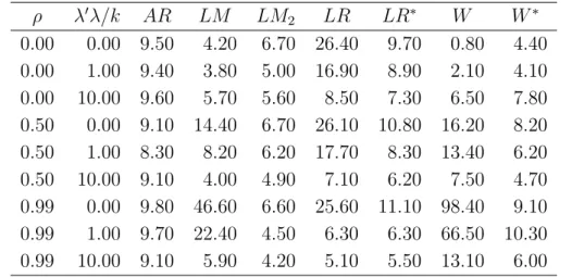
Tables II and III present rejection probabilities for the following tests: Anderson-Rubin4

(AR), the Hessian-based score test (LM) described by Zivot, Startz and Nelson (1998), the information-based score test (LM2)

described in Moreira (2001), the likelihood ratio test (LR), the conditional likelihood ratio test (LR∗₎_, _{the Wald test centered around the 2SLS}

estima-tor (W), and the conditional Wald test (W∗₎_. _The _AR_,_LM

2, LR∗, and W∗

tests are approximately similar, whereas the LM, LR,and W test are not. Although the LM test does not present good size properties, the LM2

test does. Likewise, the LR and W tests present worse size properties than the conditional LR∗ _and _W∗ _{tests. The null rejection probabilities of the}

LR test range from 0.048-0.220 and those of the W test range from 0.002-0.992 when the number of observations is 80. The null rejection probabilities of their conditional counterparts range from 0.046-0.075 and 0.030-0.072, respectively.

Results for non-normal disturbances are analogous5

. Tables IV and V show the rejection probabilities of some 5% tests when Staiger and Stock’s design II is used. The structural disturbances, u and v2, are serially

uncor-related with ut = (ξ12_t −1)/

√

2 and v2_t = (ξ 2

2_t −1)/

√

2 where ξ1_t and ξ2_t

are normal with unit variance and correlation √ρ. The k instruments are indicator variables with equal number of observations in each cell. When the number of observations is 80, the rejection probabilities underH0 of theLR∗

and W∗ _{tests are still close to 5% for all values of} _λ′_λ/k _and _ρ_.

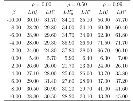
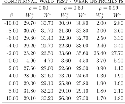
Finally, Tables VI and VII compare the power of the conditionalLR∗

0 test 4

For theARtest, aχ2

(k) critical value was used.

5

(13)

(Ω known) with that of the conditional LR∗ _{test (Ω unknown) when Staiger}

and Stock’s design I with 100 observations is used. The difference between the two power curves is small, which suggests that the power comparison in Section 2.3 for theLR∗

0 test is also valid for theLR∗ test. Tables VIII and IX

show that the same conclusion holds for the conditional W∗

0 and W∗ tests.

4 Extensions

The previous theory can easily be extended to a structural equation with more than two endogenous variables and with additional exogenous variables as long as inference is to be conducted on all the endogenous coefficients. Consider the structural equation

y1 =Y2β+Xγ+u

whereY2 is then×l matrix of observations on thel explanatory endogenous

variable and X is the n_×r matrix of observations onr exogenous variables. This equation is part of a larger linear system containing the additional exogenous variables Z. The reduced form forY = [y1, Y2] is

y1 = ZΠβ+Xδ+v1

Y2 = ZΠ +XΓ +V2

where δ= Γβ+γ. The rows ofV = [v1, V2] are i.i.d. normal random vectors

with mean zero and covariance matrix Ω. It is assumed that X and Z have full column rank. The problem is to test the vector hypothesis H0 :β =β0

treating Π, Γ, δ as nuisance parameters.

The unknown parameters associated with X can be eliminated by tak-ing orthogonal projections. Define the l+ 1 component column vector b = (1,₋β′

0)′. Let A be any (l+ 1)×l matrix whose columns are orthogonal to

b. Then, if MX =I−X(X′X)−1X′, the statistics

S=Z′_M

XY b and T =Z′MXYΩ−

1

(14)

are independent and normally distributed. For a nonpivotal statisticψ(S, T, β0),

the critical value can be found computing the 1₋α quantile of the distribu-tion of ψ conditioned on T =t. Again, Ω can be replaced with a consistent estimate and the normality assumption dropped without affecting the results significantly.

5 Confidence Regions

Confidence regions for β with approximately correct coverage probability can be constructed by inverting approximately similar tests. Although Du-four (1997) showed that Wald-type confidence intervals are not valid, the confidence regions based on the conditional Wald test has correct coverage probability in large samples no matter how weak the instruments. Likewise, if the LM2 test or the conditional LR test is used, the resulting confidence

regions have approximately correct level. Moreover, the regions based on the conditional Wald test necessarily contain the 2SLS estimator of β while the ones based on the conditional likelihood ratio test or on the LM2 test are

centered around the limited-information maximum likelihood estimator ofβ. Therefore, confidence regions based on these tests can be used as evidence of the accuracy of their respective estimators.

To illustrate how informative the confidence regions based on the condi-tional LR test are compared with the ones based on the LM2 test, design I

of Staiger and Stock (1997) is once more used. One sample was drawn where the true value of β is zero. Figures 4-6 plots the LR and LM2 statistics and

their respective critical value functions at significance level of 5% against

β0 6

. The region in which each statistic is below its critical value curve is the corresponding confidence set.

When the instruments are invalid (Figure 4), the confidence regions cover the real line. This is expected to happen about 95% of time since the confi-dence regions have correct coverage probability and β is unidentified. As the quality of the instruments increases, the confidence regions become narrower.

6

(15)

Moreover,LRconfidence regions are significantly smaller than theLM2 ones,

as a result of better power properties of the conditional likelihood ratio test. For example, when λ′_λ/k _{= 10 and} _ρ _{= 0, the} _LR _{confidence region is the}

set [0.0,0.6] while theLM confidence region is the set [₋4.1,₋2.3]_∪[0.0,0.6] (Figure 6). This illustrates that the score test fails to reject values very far from the true value, whereas the conditional likelihood ratio test does not.

6 Conclusions

Monte Carlo simulations suggest that the conditional likelihood ratio test has good size and power properties. If identification is good, this test has power curve essentially equal to the upper bound power curve for similar tests. Monte Carlo simulations also suggest that this test dominates the test proposed by Anderson and Rubin (1949) and the score tests studied by Kleibergen (2000) and Moreira (2001). This test can also be used to construct informative confidence regions with correct coverage probability centered around the limited-information maximum likelihood estimator.

The conditional approach used in this paper for finding similar tests based on nonpivotal statistics can be applied to other statistical problems involv-ing nuisance parameters. Improved inference should be possible whenever a subset of the statistics employed to form a test statistic has a nuisance-parameter free distribution and is independent of the remaining statistics under the null hypothesis.

(16)

7 References

Anderson, T., and H. Rubin (1949): “Estimation of the Parameters of a Single Equation in a Complete System of Stochastic Equations,”Annals of Mathematical Statistics, 20, 46-63.

Bound, J., D. Jaeger and R. Baker(1995): “Problems with instru-mental variables estimation when the correlation between the instruments and the endogenous explanatory variables is weak,” Journal of American Statistical Association, 90, 443-50.

Dufour, J-M. (1997): “Some impossibility theorems in econometrics with applications to structural and dynamic models,” Econometrica, 65, 1365-88.

Garderen, K. J. van (2000): “An alternative comparison of classi-cal tests: assessing the effects of curvature” in Applications of Differential Geometry to Econometrics, ed. by M. Salmon and P. Marriot. Cambridge: Cambridge University Press.

Kleibergen, F.(2000): “Pivotal Statistics for Testing Structural Pa-rameters in Instrumental Variables Regression,” Tinbergen Institute Discus-sion Paper TI2000-055/4.

Lehmann, E.(1986): Testing Statistical Hypothesis. 2nd edition, Wiley Series in Probability and Mathematical Statistics.

Moreira, M.(2001): Tests with Correct Size when Instruments Can Be Arbitrarily Weak. Manuscript.

Staiger, D., and J. Stock(1997): “Instrumental variables regression with weak instruments,” Econometrica, 65, 557-86.

Wang, J., and E. Zivot(1998): “Inference on a structural parameter in instrumental variables regression with weak instruments,” Econometrica, 66, 1389-404.

(17)

Table i

Critical Value Function of the likelihood ratio Test

k

¯

t′¯_t ₁ ₂ ₃ ₄ ₅ ₆ ₇ ₈

(18)

Table i (continued)

Critical Value Function of the likelihood ratio Test

k

¯

t′¯_t ₉ ₁₀ ₁₅ ₂₀ ₂₅ ₅₀ ₁₀₀ ₂₀₀

(19)

Table ii

Percent Rejected Under H0 at Nominal Level of 5% (20 obs.)

ρ λ′_λ/k _AR _LM _LM

2 LR LR∗ W W∗

0.00 0.00 9.50 4.20 6.70 26.40 9.70 0.80 4.40 0.00 1.00 9.40 3.80 5.00 16.90 8.90 2.10 4.10 0.00 10.00 9.60 5.70 5.60 8.50 7.30 6.50 7.80 0.50 0.00 9.10 14.40 6.70 26.10 10.80 16.20 8.20 0.50 1.00 8.30 8.20 6.20 17.70 8.30 13.40 6.20 0.50 10.00 9.10 4.00 4.90 7.10 6.20 7.50 4.70 0.99 0.00 9.80 46.60 6.60 25.60 11.10 98.40 9.10 0.99 1.00 9.70 22.40 4.50 6.30 6.30 66.50 10.30 0.99 10.00 9.10 5.90 4.20 5.10 5.50 13.10 6.00

Table iii

ρ λ′_λ/k _AR _LM _LM

2 LR LR∗ W W∗

(20)

Table iv

nonnormal disturbances and binary instruments

-ρ λ′_λ/k _AR _LM _LM

2 LR LR∗ W W∗

0.00 0.00 12.60 6.40 8.40 27.60 13.60 2.40 5.40 0.00 1.00 10.70 5.40 6.80 25.70 10.90 2.10 5.00 0.00 10.00 11.30 8.70 8.50 13.60 11.30 6.90 8.30 0.50 0.00 10.00 8.70 8.30 25.30 12.40 5.60 5.50 0.50 1.00 9.10 6.30 6.80 22.70 10.30 5.50 3.90 0.50 10.00 9.10 7.90 7.60 12.70 9.30 7.40 7.70 0.99 0.00 14.30 48.60 10.70 30.70 15.50 97.50 12.80 0.99 1.00 10.10 27.90 10.20 12.30 11.90 81.00 7.50 0.99 10.00 12.30 12.50 9.50 11.00 10.90 27.60 4.70

Table v

nonnormal disturbances and binary instruments

-ρ λ′_λ/k _AR _LM _LM

2 LR LR∗ W W∗

(21)

Table vi

Percent Rejected at Nominal Level of 5% conditional likelihood ratio test - weak instruments

ρ= 0.00 ρ= 0.50 ρ = 0.99

β LR∗

0 LR∗ LR∗0 LR∗ LR∗0 LR∗

-10.00 30.10 31.70 34.20 35.10 56.90 57.70 -8.00 28.20 29.80 34.00 34.10 60.30 60.40 -6.00 28.90 29.60 34.70 34.90 62.30 61.80 -4.00 28.00 29.30 35.90 36.90 71.50 71.70 -2.00 24.00 24.80 37.80 38.00 96.70 96.10 0.00 5.40 5.70 5.90 6.40 6.30 7.00 2.00 26.60 26.00 21.70 23.30 24.90 26.10 4.00 27.10 28.00 25.60 26.00 33.70 33.80 6.00 29.00 31.40 27.60 28.90 37.00 37.20 8.00 30.50 30.90 30.20 29.70 41.00 41.60 10.00 28.80 30.50 28.20 30.10 43.20 45.00

Table vii

Percent Rejected at Nominal Level of 5%

conditional likelihood ratio test - Good Instruments

ρ= 0.00 ρ= 0.50 ρ= 0.99

β LR∗

0 LR∗ LR0∗ LR∗ LR∗0 LR∗

-10.00 99.80 99.80 100.00 100.00 100.00 100.00 -8.00 99.70 99.80 100.00 100.00 100.00 100.00 -6.00 98.90 98.70 100.00 100.00 100.00 100.00 -4.00 95.10 95.10 100.00 99.90 100.00 100.00 -2.00 58.50 59.00 78.90 78.90 98.40 98.60

0.00 5.40 5.90 5.30 5.50 6.40 7.00

(22)

Table viii

Percent Rejected at Nominal Level of 5% conditional Wald test - weak instruments

ρ= 0.00 ρ= 0.50 ρ = 0.99

β W∗

0 W∗ W0∗ W∗ W0∗ W∗

-10.00 29.70 30.70 30.40 30.80 2.00 2.80 -8.00 30.70 31.70 31.30 32.80 2.00 2.60 -6.00 29.80 31.40 32.30 32.70 2.50 3.30 -4.00 29.20 29.70 32.30 33.00 2.40 2.40 -2.00 25.20 26.50 33.60 35.60 25.40 27.70 0.00 4.90 4.70 3.60 4.50 3.70 5.20 2.00 27.50 28.00 22.60 22.50 0.90 1.10 4.00 28.00 30.60 23.70 24.60 1.30 1.90 6.00 29.30 29.10 25.80 25.80 1.90 1.90 8.00 31.80 32.20 29.10 29.10 1.80 2.10 10.00 29.10 30.20 26.30 27.50 1.70 1.80

Table ix

Percent Rejected at Nominal Level of 5% conditional Wald test - good instruments

ρ= 0.00 ρ= 0.50 ρ= 0.99

β W∗

0 W∗ W0∗ W∗ W0∗ W∗

-10.00 99.80 99.90 100.00 100.00 100.00 100.00 -8.00 100.00 100.00 100.00 100.00 100.00 100.00 -6.00 99.70 99.40 100.00 100.00 100.00 100.00 -4.00 97.30 97.40 100.00 100.00 100.00 100.00 -2.00 70.20 69.90 73.60 74.10 43.70 43.80

0.00 5.50 5.60 4.30 4.50 5.00 5.40

(23)

Figure 1

Critical Value Function for k=4

0 1 2 3 4 5 6 7 8 9 10

3 4 5 6 7 8 9 10

||t||

Critical values

Upper bound Switching based on pre−testing Critical value function Curve−fitting

(24)

Figure 2

Empirical Power of Tests: Weak Instruments

−100 −8 −6 −4 −2 0 2 4 6 8 10

0.1 0.2 0.3 0.4 0.5 0.6 0.7

λ‘λ /k = 1, p = 0

β minus βo

Power

Power Envelope ARo test LMo test LRo* test Wo* test

Student Version of MATLAB

−100 −8 −6 −4 −2 0 2 4 6 8 10

0.1 0.2 0.3 0.4 0.5 0.6 0.7

λ‘λ /k = 1, p = 0.5

β minus βo

Power

−100 −8 −6 −4 −2 0 2 4 6 8 10

0.1 0.2 0.3 0.4 0.5 0.6 0.7 0.8 0.9 1

λ‘λ /k = 1, p = 0.99

β minus βo

Power

(25)

Figure 3

Empirical Power of Tests: Good Instruments

−2 −1.5 −1 −0.5 0 0.5 1 1.5 2

0 0.1 0.2 0.3 0.4 0.5 0.6 0.7 0.8 0.9 1

λ‘λ /k = 10, p = 0

β minus βo

Power Power Envelope ARo test LMo test LRo* test Wo* test

−2 −1.5 −1 −0.5 0 0.5 1 1.5 2

0 0.1 0.2 0.3 0.4 0.5 0.6 0.7 0.8 0.9 1

λ‘λ /k = 10, p = 0.5

β minus βo

Power Power Envelope ARo test LMo test LRo* test Wo* test

−2 −1.5 −1 −0.5 0 0.5 1 1.5 2

0 0.1 0.2 0.3 0.4 0.5 0.6 0.7 0.8 0.9 1

λ‘λ /k = 10, p = 0.99

β minus βo

(26)

Figure 4

confidence regions: Invalid Instruments

−100 −8 −6 −4 −2 0 2 4 6 8 10

1 2 3 4 5 6 7 8 9 10

λ‘λ /k = 0, p = 0

β

LR

LM2 statistic LM2 critical value LR statistic LR critical value

−100 −8 −6 −4 −2 0 2 4 6 8 10

1 2 3 4 5 6 7 8 9 10

λ‘λ /k = 0, p = 0.5

β

LR

−100 −8 −6 −4 −2 0 2 4 6 8 10

1 2 3 4 5 6 7 8 9

λ‘λ /k = 0, p = 0.99

β

LR

(27)

Figure 5

confidence regions: Weak Instruments

−100 −8 −6 −4 −2 0 2 4 6 8 10

1 2 3 4 5 6 7 8 9 10

λ‘λ /k = 1, p = 0

β

LR

−100 −8 −6 −4 −2 0 2 4 6 8 10

1 2 3 4 5 6 7 8

λ‘λ /k = 1, p = 0.5

β

LR

−100 −8 −6 −4 −2 0 2 4 6 8 10

20 40 60 80 100 120 140

λ‘λ /k = 1, p = 0.99

β

LR

(28)

Figure 6

confidence regions: Good Instruments

−100 −8 −6 −4 −2 0 2 4 6 8 10

5 10 15 20 25 30 35 40 45

λ‘λ /k = 10, p = 0

β

LR

−100 −8 −6 −4 −2 0 2 4 6 8 10

5 10 15 20 25 30 35 40 45

λ‘λ /k = 10, p = 0.5

β

LR

−100 −8 −6 −4 −2 0 2 4 6 8 10

50 100 150 200 250 300

λ‘λ /k = 10, p = 0.99

β

LR

(29)

8 Appendix A: Likelihood Ratio Derivation

Ignoring an additive constant, the log-likelihood function can be written as:

(A.1) l(Y;β, π,Ω) =₋n

2ln|Ω| − 1 2tr

¡

Ω−1

V′_V¢

Maximizing with respect toπ, one finds thatπ(β,Ω) = (Z′_Z₎−1_Z′_Y_Ω−1

c/c′_Ω−1

c

where c_≡(β ,1)′_{. The concentrated log-likelihood function,}_l

c(Y;β,Ω),

de-fined as l(Y;β, π(β,Ω),Ω), is given by:

lc(Y;β,Ω) =−

n

2ln|Ω| − 1 2

·

trΩ−1

Y′_Y ₋ c′Ω−

1

Y′_{N Y}_Ω−1

c c′_Ω−1

c

¸

When evaluated at ˆβ, the maximum likelihood estimator of β when Ω in known, this becomes

lc(Y; ˆβ,Ω) =−

n

2ln|Ω| − 1 2

£

trΩ−1

Y′_Y ₋_λ¯max¤

where ¯λmax

is the largest eigenvalue of (Z′_Z₎−1_/2

Z′_Y_Ω−1

Y′_Z₍_Z′_Z₎−1_/2

or, equivalently, the largest eigenvalue of Ω−1_/2

Y′_N

ZYΩ−1/2. Since the likelihood

ratio statistic when Ω is known,LR0, is defined as 2

h

lc

³

Y; ˆβ,Ω´₋lc(Y;β0,Ω)

i

, it follows that:

LR0 = ¯λ max

− a

′_Ω−1

Y′_N

ZYΩ−1a

a′_Ω−1

a

To find the likelihood ratio when Ω is unknown, we maximize (A.1) with respect to Ω, obtaining Ω (β, π) = V′_{V /n}_{. Inserting this into (A.1). we}

obtain

l(Y;β, π,Ω (β, π)) =₋n 2ln|V

′_V_|₊_n_{ln (}_n₎₋_n

After considerable algebra we find that the maximum value of the log-likelihood function for a fixed β is given by:

−n 2ln

µ

u′_u

u′_M

Zu

¶

− n 2ln|Y

′_M

ZY|+nln (n)−n

The concentrated log-likelihood function,lc(Y;β), defined asl(Y;β, π(β),Ω (β)),

is then given by:

lc(Y;β) = −

n

2 ln

µ

1 + d

′_Y′_N

ZY d

d′_Y′_M_Z_{Y d}

¶

− n₂ ln_|Y′_M

(30)

whered = (1,₋β)′_{. Moreover, the concentrated log-likelihood function}

eval-uated at the maximum likelihood estimator βLIM L is then given by:

lc(Y;βLIM L) =−

n

2ln

µ

1 + λ

min

n₋k

¶

− n₂ln_|Y′_M

ZY|+nln (n)−n

Since theLRwhen Ω is unknown is defined as 2 [lc(Y;βLIM L)−lc(Y;β0)],

it follows that:

LR =₋nln

µ

1 + λ

min

n₋k

¶

+nln

µ

1 + b

′_Y′_N

ZY b

b′_Y′_M

ZY b

¶

9 Appendix B: Proof of Propositions

Proof of Proposition 1: In fact we need only assume thatψ(S, t, β0)

is a continuous random variable for alltexcept for a set having T-probability zero. For any t whereψ(S, t, β0) is not a continuous random variable, define

cα(t) to be zero. Otherwise, let cα(t) be the 1−α quantile of ψ. Then, by

definition, Pr[ψ(S, T, β0) > c_α(T)|T = t] = α. Since this holds for all t, it

follows that Pr[ψ(S, T, β0)> c_α(T)] = α unconditionally.

Q.E.D.

Proof of Proposition 2: By a linear change of variables, the system (2) can be transformed into one where Ω andZ′_Z _{are identity matrices. The}

new parameter ¯β is related to the old parameter by ¯β = (βω22−ω12)/|Ω| 1_/2

.

In the new coordinates, we have

Z′_y

1 = (S+ ¯β0T)/(1 + ¯β 2 0)

Z′_y

2 = (T −β¯0S)/(1 + ¯β 2 0)

Then

¡_¯

b2_SLS−β¯0

¢2

y′

2NZy2 =

( ¯β0S′S−T′S) 2

T′_T _{+ ¯}_β2

0S′S−2 ¯β0S′T

and

¯_b2_SLS =

¯

β0(T′T −S′S) + (1−β¯ 2 0)T′S

T′_T _{+ ¯}_β2

(31)

Substituting into (3),we findW0 →S′T(T′T)− 1

T′_S/_{(1+ ¯}_β2

0) asT′T → ∞,

But S/(1 + ¯β2 0)

1_/2

is distributed as N(0,I) under the null hypothesis. Hence, conditional on T =t, W0 tends to a chi-square-one random variable. When

T = 0, W0 =S′Sβ¯ 2

0/(1 + ¯β 2

0). Transforming back to the original coordinates,

we find that this is ρ2

0/(1−ρ 2

0) times a chi-square-k random variable.

Q.E.D.

Proof of proposition 3: Note that ( ¯S,T¯) = (Z′_Z₎−1_/2

Z′_Y_Ω−1_/2

W

where

W =

·

Ω1_/2

b

√

b′_Ω_b,

Ω−1_/2

a

√

a′_Ω−1

a

¸

is an orthogonal matrix. Thus the eigenvalues of Ω−1_/2

Y′_N

ZYΩ−

1_/2

are the same as the eigenvalues of ( ¯S,T¯)′_{( ¯}_S,_T¯₎_._{The largest eigenvalue then is given}

by ¯ λmax = 1 2 · ¯

T′_T¯_{+ ¯}_S′_S¯₊

q

( ¯T′_T¯_{+ ¯}_S′_S¯₎2

−4[ ¯S′_S¯_·_T¯′_T¯₋_{( ¯}_S′_T¯₎2

]

¸

Moreover, a′_Ω−1

Y′_{N Y}_Ω−1

a/a′_Ω−1

a= ¯T′_{T .}¯ _{Therefore, the} _LR₀ _{test statistic}

is given by expression (5). For ¯T′_T¯₆_{= 0,} _LR

0 can be rewritten as

LR0 =

1 2

·

Q1+Q_k₋1−T¯′T¯+

q¡

Q1+Q_k₋1+ ¯T′T¯

¢2

−4Qk−1·T¯′T¯

¸

where Q1 = ¯S′T¯( ¯T′T¯)− 1¯

T′_S¯ _and _Q

k−1 = ¯S′[I−T¯( ¯T′T¯)− 1¯

T′_{] ¯}_S. _Conditioned

on ¯T = ¯t , Q1 and Q_k₋1 are independent and under H0 have chi-square

distributions with one and k₋1 degrees of freedom, respectively. Therefore the critical value function just depends on k, α, and ¯t′¯_t_{. When ¯}_T _{= 0}_{, LR}

0

= ¯S′_S¯_{, which is a chi- square-}_k _{random variable. When ¯}_T′_T¯ _{→ ∞}_{, LR}

0 →

( ¯S′_T¯₎2

/T¯′_T¯_{, which is a chi-square-one random variable.}