Allelic richness following population founding events--a stochastic modeling framework incorporating gene flow and genetic drift.

(1)

Allelic Richness following Population

Founding Events – A Stochastic Modeling

Framework Incorporating Gene Flow and

Genetic Drift

Gili Greenbaum1,2*, Alan R. Templeton3,4, Yair Zarmi1, Shirli Bar-David2

1.Department of Solar Energy and Environmental Physics, The Jacob Blaustein Institutes for Desert Research, Ben-Gurion University of the Negev, Midreshet Ben-Gurion, Israel,2.Mitrani Department of Desert Ecology, The Jacob Blaustein Institutes for Desert Research, Ben-Gurion University of the Negev, Midreshet Ben-Gurion, Israel,3.Department of Biology, Washington University, St. Louis, Missouri, United States of America,4.Institute of Evolution, and Department of Evolutionary and Environmental Biology, University of Haifa, Haifa, Israel

*[email protected]

Abstract

Allelic richness (number of alleles) is a measure of genetic diversity indicative of a population’s long-term potential for adaptability and persistence. It is used less commonly than heterozygosity as a genetic diversity measure, partially because it is more mathematically difficult to take into account the stochastic process of genetic drift for allelic richness. This paper presents a stochastic model for the allelic richness of a newly founded population experiencing genetic drift and gene flow. The model follows the dynamics of alleles lost during the founder event and simulates the effect of gene flow on maintenance and recovery of allelic richness. The probability of an allele’s presence in the population was identified as the relevant statistical property for a meaningful interpretation of allelic richness. A method is discussed that combines the probability of allele presence with a population’s allele frequency spectrum to provide predictions for allele recovery. The model’s analysis provides insights into the dynamics of allelic richness following a founder event, taking into account gene flow and the allele frequency spectrum. Furthermore, the model indicates that the ‘‘One Migrant per Generation’’ rule, a commonly used conservation guideline related to heterozygosity, may be inadequate for addressing preservation of diversity at the allelic level. This highlights the importance of distinguishing between heterozygosity and allelic richness as measures of genetic diversity, since focusing merely on the preservation of heterozygosity might not be enough to adequately preserve allelic richness, which is crucial for species persistence and evolution. OPEN ACCESS

Citation:Greenbaum G, Templeton AR, Zarmi Y, Bar-David S (2014) Allelic Richness following Population Founding Events – A Stochastic Modeling Framework Incorporating Gene Flow and Genetic Drift. PLoS ONE 9(12): e115203. doi:10. 1371/journal.pone.0115203

Editor:Lilach Hadany, Tel Aviv University, Israel

Received:June 19, 2014

Accepted:November 19, 2014

Published:December 19, 2014

Copyright:ß_{2014 Greenbaum et al. This is an}

open-access article distributed under the terms of theCreative Commons Attribution License, which permits unrestricted use, distribution, and repro-duction in any medium, provided the original author and source are credited.

Data Availability:The authors confirm that all data underlying the findings are fully available without restriction. All relevant data are within the paper and its Supporting Information files.

Funding:GG fellowship was supported by the 2010 SIDEER (Swiss Institute for Dryland Environmental and Energy Research) Fund for interdisciplinary research. The funders had no role in study design, data collection and analysis, decision to publish, or preparation of the manuscript.

(2)

Introduction

Genetic diversity is an important aspect of the dynamics of populations, as it is directly related to the evolutionary potential of the population and the deleterious effects of inbreeding [1]. There are, however, several different types of measures of genetic diversity, most notably measures based on heterozygosity and measures based on allelic richness (defined as the number of alleles). These groups of measures differ in their formulations, their ecological and evolutionary

interpretations, and the mathematical frameworks in which they can be applied [2–4].

Observed heterozygosity (HO), the frequency of heterozygous individuals in a

population, or expected heterozygosity (HE), the probability that two gametes,

randomly chosen from the gene pool, are of different alleles, are by far the measures most commonly used by the majority of papers that present a genetic summary of populations [4] (e.g., [5,6]). These measures are very sensitive to the allele frequencies in the population, rather than just to the number of alleles. It has been shown that a decrease in the observed heterozygosity can induce a decrease in the average fitness of individuals [7,8], and thus this measure has clear ecological consequences. There exists an extensive mathematical framework, F-statistics, first presented by Wright [9], that allows for the modeling and analysis of varied scenarios regarding heterozygosity, as well as the inclusion of processes such as gene flow to provide quantitative predictions and assessments. Allele richness (also referred to as allelic diversity) is calculated as the average number of alleles per locus [1]. A decrease in the allelic richness could lead to a reduction in the population’s potential to adapt to future environmental changes, since this diversity is the raw material for evolution by natural selection [10]. While not all variation is related to the adaptive potential, clearly no standing variation exists if no allelic richness exists. Moreover, there is evidence that high allelic richness, even of merely neutral alleles, increases evolvability by making a larger fraction of the genotypic space accessible by fewer mutational events [11]. Allelic richness is, therefore, a strong indicator for the evolutionary potential of a population [2,3,12], and it has been suggested that this measure is of key importance in population conservation and management [13–18]. Allelic richness measures are also commonly presented in population genetic summaries (as the number of alleles in a given locus or the mean number of alleles per locus). However, in practice, conclusions pertaining to these measures are often merely comparative, such as ‘‘population A has higher allelic richness than population B’’ or ‘‘the population had higher allelic richness at time T than at time S’’, and not quantitative.

(3)

Generation’’ (OMPG) rule [12,21]. The rule states that, under the conditions of an island model of migration in which gene flow is not influenced by distance or any geographical feature, an exchange of one effective migrant per generation (effective migrants are migrants that breed and contribute to the population’s gene pool; for the purpose of this paper, all migrants will be regarded as effective migrants) is enough to adequately maintain the genetic diversity of the population [22,23]. This rule is derived from the island model [24], and other F-statistics models have been formulated (e.g., the stepping stone model [25]), but they are used less frequently as conservation guidelines.

Founder events are known to decrease the genetic diversity of the population [26], and are often followed by a demographic expansion. It has been shown, both theoretically [2,26–30] and empirically [27,31], that allelic richness is more sensitive than heterozygosity to founder events followed by expansions, since allelic richness does not consider abundances of the alleles but only their presence (a rare allele that is lost in a founder event will probably not affect heterozygosity much, but the loss does reduce allelic richness). Moreover, allelic richness is more indicative of the evolutionary potential of the population in the long-run in these scenarios [2,3,12], as the existence of alleles, rather than their frequencies, holds a significant part of potential for response to selection, as selection limits are determined by the initial allelic composition [13,32] (studied for biallelic loci by [33–35]) rather than by levels of heterozygosity. For example, consider a

population withndifferent alleles with different selection coefficients (e.g., taken randomly from a uniform distributionU(0,1)). If we consider that only selection is at play, eventually alleles with the highest selection coefficients will become abundant while the rest will be lost. Thus the eventual fitness of the population will be determined by the expected maximal value of the initial selection coefficients, a value which depends on n, the number of alleles (1{

1

nz1 in the

case of the uniform distribution above). This maximal value is higher when nis larger, and therefore, populations with higher allelic richness are expected to eventually show higher average fitness, under these assumptions. Nevertheless, most theoretical models and conservation applications pertaining to these scenarios are still drawn from the F-Statistics framework [4], where higher heterozygosity levels are considered to convey increased response to selection. While some work has been done in modeling allelic richness [36–39], the field has not yet been fully investigated.

(4)

population, with gene flow potentially generating an increase in allelic richness and genetic drift leading to a decrease.

The goal of this paper is to present a simulation framework, to be used as a method for estimating the maintenance and recovery of allelic richness, as well as for identifying the appropriate statistical properties with which to address allelic richness in similar modeling frameworks. A model was developed in a neutral theory [42,43] context that focuses on gene flow and genetic drift in a founder scenario. The model tracks and simulates a single allele lost in the founder event under different demographic parameters and allele frequencies, and later it is shown how the single-allele results can be extended and applied to the entire allele frequency spectrum to give a meaningful estimation of overall allelic richness recovery. While the model does not include mutation and selection, although they may be relevant in many scenarios, it provides insights into the potential effect of gene flow in the recovery of allelic richness. The model’s results also demonstrate that the OMPG rule may not be sufficient to conserve allelic richness, and thus they emphasize the need to distinguish between allelic richness and heterozygosity regarding management conclusions pertaining to migration rates between populations. Such conclusions should be drawn while taking both measures into account.

Methods

2.1. Model

The model consists of a source population and a newly founded population. The source population is the population from which the founded population

originated and from which migrants can possibly arrive. It is assumed to be an ideal population at Hardy-Weinberg equilibrium, much larger than the founded population, and is therefore assigned a static genetic description (i.e., allele frequencies in the population do not change over time), while the founded population is dynamic in this regard. The model tracks the frequency of a single allele in the founded population over time. The founded population is assumed to be demographically expanding with a discrete logistic equation describing the population size:

Ntz1~N_tzrN_t(1{

Nt

K ) ð1Þ

whereNtis the population size at timet,ris the population growth rate andKthe

carrying capacity (note that migration does not affect the population size).Ntwas

(5)

The model assumes a Poisson-distributed migration pattern. The mean number of migrants per generation from the source population to the founded population isMand the mean number of migrants from the founded population back to the source population is mNt (a proportionm of the population each generation).

Migration is defined to be asymmetric because we assume the source population is large and static, while the size of the founded population is dynamic (following eq. 1). Note that the inclusion of back-migration when the source population is constant could have been left out of the model, since these migrating individuals are effectively ‘‘lost’’, but it has been included in order to provide an outline for future development of the model (here we assume that the source population is very large, and therefore, the effect of back migration on the source population allele frequencies is negligible). We also used a deterministic migration pattern, in which the number of migrants per generation is constant (see S1 Appendix and

S1 andS2 Tables). Migrants are assumed to carry the allele in question according to the frequency of the allele in the population from which they are migrating.

Genetic drift is simulated according to the Wright-Fisher model [24]: a random independent draw for each gamete determines whether it is a gamete of the allele in question or not. This induces a binomial distribution on the number of gametes of the allele. The model, combining both gene flow and genetic drift, can thus be summarized as follows:

qtz1~

B(2_N_t_z₁{2_M

tz1,qt)zB(2Mtz1,Q)

2_N_t_z₁_{2_M

tz1z2Mtz1

ð2_Þ

with the initial condition q1~0. Hereq_tis the allele frequency; B(n,p) is the

Binomial distribution with n number of trials and success probabilityp;M_t, the number of migrants back-migrating to the source population at time t, is a random variable with a Poisson distributionM_t*Pois(mNt); andMt, the number

of migrants to the founded population at time t, is a random variable with a Poisson distribution Mt*Pois(M). The numerator represents the number of

alleles in the population after one generation of migration as the sum of two random variables with the first reflecting alleles drawn from the founded

population’s gene pool and the second alleles drawn from the migrants, and the denominator represents the relevant population size.

The expected value of qtis thus given by:

E q½ tz1~

E½qtNtz1(1{m)zQM Ntz1(1{m)zM

ð3_Þ

and at equilibrium, the expected value is E½qequilibrium~Q (forMw0). This

theoretical expected value should be approached when the stochastic nature of the process (i.e. genetic drift) is negligible, but otherwise, the empirical mean allele frequency at equilibrium, qequilibrium, might also depend on other parameters, due

to the absorbing boundaries of the genetic drift process at q~0 _and _q~1_.

A comprehensive theory for analytically describing qequilibrium that takes all the

(6)

approxima-tion can be used. The expected waiting time between arrival from the source

population of two individual alleles is Ta~

1

2_MQ ast??, and the expected

waiting time for an individual allele’s loss, assuming that the population is at carrying capacity (N~_K), is approximatelyTl~2 ln(2K)[44] (here an additional

assumption is made, that the allele frequency at arrival is very small compared to

K). Thus, forMw 1

4_Qln₍2_K₎, the waiting time between arrivals is shorter than the

loss time (TavTl), and we expect qequilibrium~Q to hold. Otherwise, qequilibrium is

expected to be lower in proportion to the time interval in which the allele is present:

qequilibrium~Q

Tl

Ta

~4_MQ2ln₍2_K₎

: ð4Þ

2.2. Simulations

Simulations were carried out for different scenarios with the following parameter values: initial population size N0~5,10,20; carrying capacity K~200,400,1000;

population growth rate r~0

:01,0:05,0:1. All scenarios were simulated for

frequencies in the source population of Q~0

:01 to 0.02 (0.01 intervals) and

migration rates from the source population to the founded population ofM~0 :1

to 30 (0.1 intervals). For all simulations, a fixed back-migration value ofm~0 :05

was used. These parameters were chosen to illustrate the presented framework since they could be reasonable parameters for a reintroduction of a mammalian population, as a possible application, but the framework is not restricted to these parameters.

We ran 1000 simulations for each scenario. The mean allele frequency and the probability of allele presence (see below) were calculated for each generation across the 1000 simulations. Each of these simulations was run until equilibrium was reached, plus an additional 200 generations to generate the equilibrium phase of the system (equivalent to the migration-drift balance). The equilibrium generation was defined by first defining an equilibrium separately for the mean allele frequency and for the probability of allele presence. Equilibrium was defined as the generation for which the following 100 generations show no trend, i.e., the difference between the number of generations showing a positive change in the statistical property (mean allele frequency or probability of allele presence) and the number of generations showing a negative change was one or zero. The overall equilibrium was taken as the greater of these two equilibria to ensure that the system is stable for both statistical properties. This conservative definition of equilibrium, which could overestimate the actual time needed to reach

(7)

The model focuses on time scales that are sufficiently short and on population sizes that are sufficiently small, so that mutation can be neglected; mutation events are very rare in small populations during short time scales [20]. The model was simulated using MATHEMATICA software [45], and appears in S2 Appendix

along with the code for the analysis and the graphical representation of the results (which could be used with alternative parameterizations).

2.3. Simulation analysis

Probability measures can be broken into a discrete part and a continuous part (Jordan’s decomposition theorem [46]). In the dynamics of allele frequency over time, the discrete part of the probability measure constitutes the allele frequencies 0 and 1 - the events of allele fixation and allele loss, respectively. For each of these two points, there is a positive probability that the allele has those frequencies, and we define these probabilities asp0andp1respectively. This attribution of positive

probabilities to singular points is due to the fact that the stochastic process of genetic drift has absorbing boundaries at these points, and alleles that have reached loss or fixation are expected to remain in these states for some time (permanently in the absence of gene flow or mutations). For the frequencies between but not including 0 and 1, a continuous probability distribution is an appropriate description. Thus, the behavior of the system at 0 and 1 should be considered separately from the rest of the distribution (see Fig. 1 for an

illustration, explained below). We define the ‘probability of allele presence’ as the probability of the allele not being at frequency zero:

ppresence~1{p0_: ð5Þ

The probabilityppresence was calculated for each generation in each scenario

from the simulations.

The equilibrium phase of the population was defined as the 200 generations after equilibrium was reached, and the meanppresencewas calculated over these 200

generations, as well as the mean allele frequency (the mean over 200 generations of the mean allele frequency for 1000 simulations). For a given scenario, the minimal migration rate required to reach E½qequilibrium~Q (i.e., the mean allele

frequency at equilibrium as the source population’s allele frequency) was defined as the minimal migration rate Mmean for which all qequilibrium values for

MmeanƒMvMmeanz0:05are above 0.95Q(i.e., the minimal migration for which

five consecutive data points are above 95% of the allele frequency in the source population). This was done in order to estimate how many migrants are needed to ensure that the expected mean allele frequency at equilibrium is reasonably stable around Q.

The presence of an allele in the system was defined based on a threshold - the ‘95% probability of allele presence’. Only scenarios in whichppresenceis higher than

95% (ppresencew0:95) are assumed to have the allele in question with high enough

(8)

similarly by Tracyet al.[47]). For a given scenario, the migration rate required for allele presence with 95% probability, Mpresence, was defined as the minimal

migration rate for which ppresencew0:95. Both Mmean and Mpresence were obtained

for all scenarios and for Qvalues of 0.02, 0.04, 0.1 and 0.2.

2.4. Source population allele frequency spectrum

In order to assess the model’s implications for a polymorphic locus and not just a single allele, the allele frequency spectrum of the source population is compared with results for simulations with differentQvalues. To illustrate this process, and the application of the model with allele frequency spectra, examples of theoretical frequency spectra for the source population were generated using the method presented by Ewens [48]:

E(x1,x2)~h ð

x2

x1

(1_{_x₎h{1

x dxf or

1

2_N_evƒx1ƒx2ƒ1h~4Nevm: ð6Þ

This equation allows for the calculation of the expected number of alleles with frequencies betweenx1 andx2, wherem is the mutation rate andN_evthe variance

effective population size of the source population. Nev~5000 (although the

population is assumed large, a finite Nevwas used in order to derive an

equilibrium allele frequency spectrum) and three different mutation rates,

m~5|10{6

,5|10{5

,5|10{4

(resulting inh~0

:1,1,10, respectively), were

taken to represent the source population. These per locus mutation rates correspond to the estimated range of human mutation rates [49,50]. The resulting frequency spectra appear in Fig. 2.

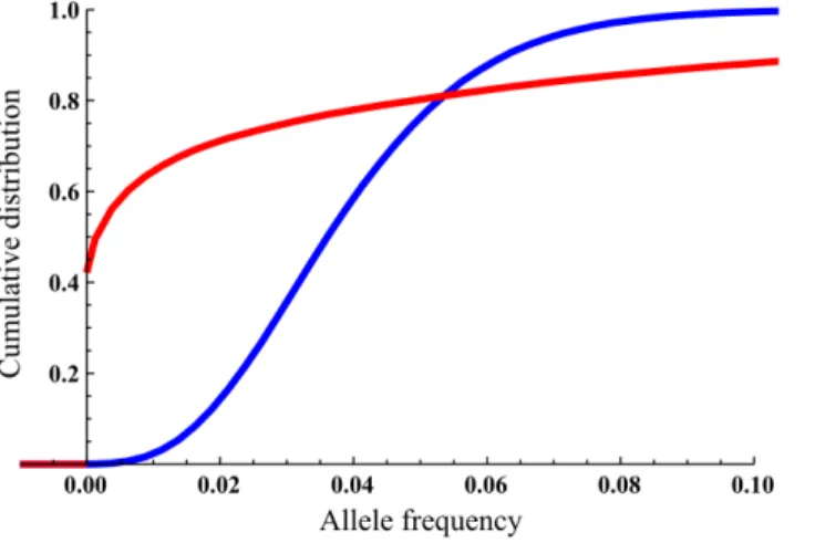
Fig. 1. Cumulative density functions for the allele frequency at the equilibrium phase.M~1migrants in blue,M~30migrants in red; scenario parametersQ~0

:04,N0~10,K~400,r~0:05,m~0:05. The jump at allele frequency 0 forM~1is due to the lowppresencefor this scenario.

(9)

The ‘95% probability of allele presence’, as described above, was similarly used to obtain a ‘cut-off frequency’, Qc, a threshold frequency (in the source

population) above which the allele in question is assumed to be present in the population (i.e., ppresencew0:95). The cut-off frequency of a given scenario was

then compared with the allele frequency spectra in Fig. 2, and the number of alleles above the cut-off frequency was calculated using eq. 6, i.e. E(Qc,1), as well

as their proportion from the overall expected number of alleles, i.e. E(Qc,1) E( 1

2_N_ev,1)

.

The cut-off frequency and the number and proportion of alleles that are potentially expected to be recovered by gene flow (with the 95% probability guideline), if lost in a founder effect, were calculated for three different migration rates, M~1_, _M~5 _and_M~20_.

Results

In all simulated scenarios, the mean allele frequency in the founded population increased over time, showing eventual stabilization. The same pattern was observed for ppresence. The number of migrants required for the mean allele

frequency at equilibrium (qequilibrium) to recover to the same mean frequency as in

the source population, Mmean, varied between 0.2 to 4.9 migrants per generation,

with most scenarios requiring between 0.5–2.5 migrants, summarized in Table 1

(average over all scenarios simulated of1

:48+0:91migrants). For migration rates

below Mmean, the mean frequency at equilibrium was lower than Q, with an

example shown in Fig. 3 (all results are presented in S1–S9 Figs.).Mmean values

were generally higher for rare alleles (Q~0

:02 and 0.04), compared with more

common alleles (Q~0

:1 and 0.2), with averages of 1.74¡0.98 migrants, and 1

:22+0:75 migrants respectively. Mmean values were also generally higher for

larger initial population sizes, higher carrying capacities and higher growth rates (Table 1).

While the simplified approximation summarized byequation 4was far from an accurate evaluation of qequilibrium for migration rates below Mmean, it did

Fig. 2. Theoretical allele frequency spectra.Theoretical allele frequency spectra for A)h~0_:1(blue); B)h~1(red); C)h~10(green). The frequency spectra were generated usingequation 6.

(10)

qualitatively describe the gradual increase inqequilibriumfor migration rates below a

threshold and stabilization of Q(S1–S9 Figs.). A better approximation was attained using a regression analysis with the model Q(1{_e{aM)with unknown parameter aintroduced to increase the goodness of fit of the model, shown inS1–S9 Figs., and with regression details presented inS3 Table. For the scenarios simulated,Mmean was estimated fairly well byequation 4for rare alleles, but less so

for more common alleles. The simplified approximation also showed migration thresholds for stabilization that were higher for common alleles, compared with Table 1.MmeanandMpresencethresholds for different scenarios.

Mmean Mpresence

N0 r K Q~0:02 Q~0:04 Q~0:1 Q~0:2 Q~0:02 Q~0:04 Q~0:1 Q~0:2

5 0.01 200 1.2 0.6 0.2 0.2 26.8 11.7 2.1 1.0

400 0.7 1.4 0.4 0.2 30.4 5.9 1.9 0.8

1000 0.8 0.4 0.6 0.2 16.6 10.8 2.0 0.7

0.05 200 1.8 1.2 0.6 0.7 17.4 6.3 1.9 0.8

400 2.2 0.4 0.5 1.0 12.5 5.0 1.6 0.8

1000 1.9 0.8 0.7 0.8 9.1 3.8 1.3 0.6

0.1 200 0.9 0.9 1.2 0.6 17.8 6.3 1.9 0.8

400 1.4 1.7 1.4 1.2 12.4 4.9 1.6 0.8

1000 1.3 2.5 1.3 1.5 9.3 3.9 1.4 0.7

10 0.01 200 1.8 1.1 0.7 1.3 19.8 7.7 2.5 0.9

400 1.0 0.4 0.7 0.5 15.7 10.4 1.9 0.8

1000 1.0 0.5 0.5 0.3 13.0 4.7 1.8 1.0

0.05 200 1.6 1.9 1.3 1.0 17.3 6.4 1.9 0.8

400 1.9 1.3 1.4 1.2 12.9 4.9 1.6 0.8

1000 2.0 1.5 1.5 1.5 9.2 4.0 1.3 0.7

0.1 200 1.9 1.8 1.1 0.9 17.5 6.2 1.9 0.9

400 2.9 2.7 2.0 1.9 12.7 4.9 1.6 0.8

1000 2.7 2.4 2.4 2.4 9.0 3.8 1.4 0.7

20 0.01 200 1.0 1.3 0.8 0.6 21.6 6.9 2.3 0.9

400 0.8 0.7 0.8 1.0 15.8 7.3 1.8 0.8

1000 1.8 1.7 1.1 0.7 15.2 4.0 1.7 0.7

0.05 200 1.5 2.3 2.2 1.6 17.2 6.2 1.9 0.9

400 2.0 2.9 2.2 1.8 12.7 4.9 1.6 0.8

1000 2.3 3.3 2.5 2.1 9.0 3.8 1.4 0.7

0.1 200 1.9 2.0 1.3 0.9 17.5 6.4 1.9 0.8

400 4.1 2.5 2.6 1.4 12.6 5.0 1.7 0.7

1000 4.6 4.9 3.3 3.1 9.0 3.9 1.4 0.7

Parameters: initial population size (N0); growth rate (r); carrying capacity (K); source population allele frequency (Q); minimal number of

migrants from source population to founded population required to reach mean allele migrants from source population to founded

doi:10.1371/journal.pone.0115203.t001

(11)

rare alleles, a pattern similar to that shown by the Mmean values from the

simulations.

The migration thresholds when considering mean allele frequency and when considering the probability of allele presence were considerably different, as can be seen inTable 1. Althoughqequilibrium wa, s similar for migration rates aboveMmean,

the actual probability distribution of the allele frequency revealed a different picture. For example, in Fig. 1, one can see very different distributions for the allele frequency at the equilibrium phase for two simulations with migration rates M~1 _and _M~30 _{(other parameters:} _Q~0

:04,N0~10,r~0:05K~400,

m~0

:05). Specifically, the probability of allele presence with one migrant per

generation was ppresence~0:58, evident in the large discontinuous ‘‘jump’’ in the

cumulative distribution function at allele frequency 0, while the probability for presence with 30 migrants per generation was much higher, withppresence~0:99. In

contrast, the mean allele frequency values at equilibrium for these two migration rates were almost identical, withqequilibrium~0:038forM~1andqequilibrium~0:039

for M~30_.

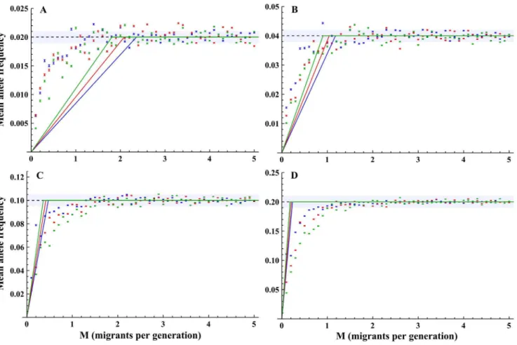
Fig. 3. Mean allele frequencies at equilibrium(qequilibrium)as a function of the number of migrants per generation.Solid lines indicate the estimation of

the mean allele frequency (equation 4), dashed lines indicateMmeanthresholds.K~200in blue;K~400in red;K~1000in blue. A)Q~0:02; B)Q~0:04; C)

Q~0_:1; D)Q~0_:2. Scenario parameters:N0~10,r~0:05,m~0:05. Error bars indicate the standard error of the mean.

(12)

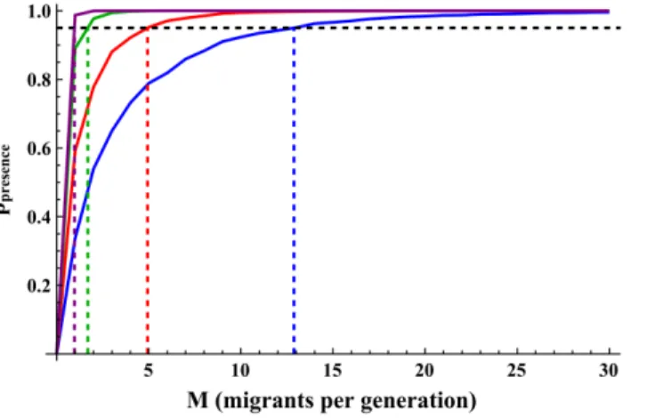
Fig. 4 shows the Mpresence thresholds (number of migrants required to reach

ppresencew0:95) for four scenarios, and Table 1summarizes the thresholds for all

scenarios simulated. Evidently,Mpresencethresholds were very much affected by the

source population allele frequency and were much higher for rare alleles than for more common alleles (an average of 11

:23+6:34 for Q~0:02 and Q~0:04

compared to an average of1

:34+0:52forQ~0:1andQ~0:2). When comparing

the Mpresence andMmean thresholds, for Q~0:02,Mpresence was much larger than

Mmean for all scenarios simulated (an average Mmean of1:81+0:93 in contrast to

an averageMpresence of16:0+5:36), and forQ~0:04this was true for all scenarios

but one (an average Mmean of 1:67+1:05 in contrast to an average Mpresence of 6

:47+2:47). For the more common alleles, however, the two thresholds were

generally similar (an average Mmean of 1:22+0:74 and an averageMpresence of 1

:34+0:52 for Q~0:1 and Q~0:2 combined). In contrast to the Mmean

thresholds, the Mpresence thresholds were generally lower for higher initial sizes,

carrying capacities and growth rates; however, this was only evident for the rare alleles, while for the more common alleles,Mpresence was not much affected by the

change of scenario parameters.

3.1. Allele frequency spectrum

Performing an analysis on polymorphic loci requires attention to different alleles with different frequencies, and not just a single allele.Fig. 5shows how the cut-off frequency can be derived from the perspective of the allele frequency in the source population. For example, with K~400_,_r_~0

:1 andN0~10, and one migrant per

generation (M~1_{), alleles of frequencies} _Q_c~0

:15 or higher are expected to be

present in the founded population at equilibrium with a probability of 95% or higher, while alleles with lower frequencies are not. For the same demographic parameters, for M~5 _{the cut-off frequency is}_Q

c~0:05, and forM~20 the

cut-off frequency is Qc~0:02.

Table 2summarizes the cut-off frequencies and the proportion of allelic richness that is expected to be recovered, given the defined genetic goal of 95% probability of allele presence and the allele frequency spectra given in Fig. 2. Different migration rates result in different cut-off frequencies, and therefore have different impacts on the recovery potential of allelic richness. While the

demographic parameters of the founded population seem to have little impact on the proportion of allelic richness expected to be recovered, the allele frequency spectrum of the source population has a major effect on the potential of recovery of alleles (Qcvalues in Table 2 do not vary much with different demographic

parameters, but they do vary with differenthvalues). Allele frequency spectra that have few rare alleles (low hvalues) have more alleles above the cut-off frequency and a higher potential for recovery of allelic richness. In contrast, allele

(13)

Discussion

The model follows a single allele that is subject to two evolutionary forces: gene flow and genetic drift. If the stochastic nature of genetic drift and migration pattern are ignored, equation 3 predicts that the mean allele frequency at equilibrium, qequilibrium, should converge to the allele frequency in the source

population, Q. The observation that for the scenarios simulated, the mean allele frequency indeed converged to Qat equilibrium for high enough migration rates (Fig. 3 and S1–S9 Figs.) fits this deterministic prediction. For migration rates lower than the threshold (Mmean),qequilibrium was lower and only qualitatively

Fig. 4.ppresence(probability of allele presence) for different migration rates.Q~0:01in blue;Q~0:02in red;

Q~0_:1in green andQ~0_:2in purple. Horizontal dashed line show the 95% probability of allele presence threshold (ppresence~0:95) and vertical dashed lines showMpresencethresholds. Scenario parameters:

N0~10,r~0:05,K~400,m~0:05. standard error of the mean was below 0.002 for allppresencevalues and is therefore not indicated.

doi:10.1371/journal.pone.0115203.g004

Fig. 5. Probability of allele presence for differentQvalues (allele frequencies in source population).

M~1in blue,M~5in red andM~20in green. Horizontal dashed line show the 95% probability of allele presence threshold (ppresence~0:95) and vertical dashed lines showQcthresholds (cut-off frequencies) for the different migration rates. Scenario parameters:N0~10,r~0

:05,K~400,m~0:05.

(14)

described by the simplified approximation given in equation 4. This lower qequilibrium is due to the fact that the arrival times of the allele from the source

population are long enough, compared to the time required for the allele to be lost, so that the allele is absent for significant periods from the population.

These last observations, and the simulation results of typicalMmean values of

0.5–2.5, might lead to the erroneous conclusion that in these scenarios, migration rates higher than one or two migrants per generation are enough to restore the loss of genetic diversity for most scenarios, as the mean allele frequency in the Table 2.Proportion of allelic richness recovered by gene flow and cut-off frequencies (Qc).

M~1 _M~5 _M~20

Proportion of allelic richness recovered

N0 r K Qc h~0:1 h~1 h~10 Qc h~0:1 h~1 h~10 Qc h~0:1 h~1 h~10

5 0.01 200 0.2 0.59 0.17 0.01 0.08 0.65 0.27 0.05 0.03 0.7 0.38 0.15

400 0.16 0.6 0.2 0.01 0.05 0.67 0.33 0.09 0.03 0.7 0.38 0.15

1000 0.18 0.6 0.19 0.01 0.04 0.68 0.35 0.11 0.04 0.68 0.35 0.11

0.05 200 0.18 0.6 0.19 0.01 0.06 0.66 0.31 0.07 0.03 0.7 0.38 0.15

400 0.2 0.59 0.17 0.01 0.06 0.66 0.31 0.07 0.03 0.7 0.38 0.15

1000 0.17 0.6 0.19 0.01 0.06 0.66 0.31 0.07 0.03 0.7 0.38 0.15

0.1 200 0.17 0.6 0.19 0.01 0.06 0.66 0.31 0.07 0.03 0.7 0.38 0.15

400 0.16 0.6 0.2 0.01 0.06 0.66 0.31 0.07 0.03 0.7 0.38 0.15

1000 0.13 0.62 0.22 0.02 0.05 0.67 0.33 0.09 0.02 0.72 0.42 0.2

10 0.01 200 0.16 0.6 0.2 0.01 0.05 0.67 0.33 0.09 0.02 0.72 0.42 0.2

400 0.14 0.61 0.21 0.02 0.04 0.68 0.35 0.11 0.02 0.72 0.42 0.2

1000 0.13 0.62 0.22 0.02 0.04 0.68 0.35 0.11 0.02 0.72 0.42 0.2

0.05 200 0.17 0.6 0.19 0.01 0.05 0.67 0.33 0.09 0.02 0.72 0.42 0.2

400 0.15 0.61 0.21 0.01 0.05 0.67 0.33 0.09 0.02 0.72 0.42 0.2

1000 0.12 0.62 0.23 0.02 0.04 0.68 0.35 0.11 0.02 0.72 0.42 0.2

0.1 200 0.16 0.6 0.2 0.01 0.05 0.67 0.33 0.09 0.02 0.72 0.42 0.2

400 0.15 0.61 0.21 0.01 0.04 0.68 0.35 0.11 0.02 0.72 0.42 0.2

1000 0.13 0.62 0.22 0.02 0.04 0.68 0.35 0.11 0.02 0.72 0.42 0.2

20 0.01 200 0.16 0.6 0.2 0.01 0.05 0.67 0.33 0.09 0.02 0.72 0.42 0.2

400 0.14 0.61 0.21 0.02 0.04 0.68 0.35 0.11 0.02 0.72 0.42 0.2

1000 0.12 0.62 0.23 0.02 0.04 0.68 0.35 0.11 0.02 0.72 0.42 0.2

0.05 200 0.16 0.6 0.2 0.01 0.05 0.67 0.33 0.09 0.02 0.72 0.42 0.2

400 0.14 0.61 0.21 0.02 0.04 0.68 0.35 0.11 0.02 0.72 0.42 0.2

1000 0.13 0.62 0.22 0.02 0.04 0.68 0.35 0.11 0.02 0.72 0.42 0.2

0.1 200 0.17 0.6 0.19 0.01 0.05 0.67 0.33 0.09 0.02 0.72 0.42 0.2

400 0.14 0.61 0.21 0.02 0.04 0.68 0.35 0.11 0.02 0.72 0.42 0.2

1000 0.12 0.62 0.23 0.02 0.04 0.68 0.35 0.11 0.02 0.72 0.42 0.2 Initial population size (N0); growth rate (r); carrying capacity (K); migrants per generation from source population to founded population (M); cut-off frequency (Qc); source population allele frequency spectrum (defined byequation 6) with givenhvalue.

(15)

founded population is similar to that of the source population. This conclusion would be concordant with the analogous analysis of heterozygosity in a

migration-drift island model that is exemplified in the OMPG rule (the One Migrant Per Generation rule states that one migrant per generation is an adequate gene flow rate to prevent loss of genetic diversity). The actual probability distributions (Fig. 1) and, specifically, the probability of allele presence (Fig. 4), reveal that this is not the case for allelic richness. In the scenarios simulated, the migration rates needed to reach the defined threshold of 95% probability of presence for relatively rare alleles are typically much higher than the migration rates needed for convergence of the mean frequency to Q(Table 1). This genetic goal (95% probability of allele presence [47]) directly addresses the question of the presence or the absence of the allele and is, therefore, a more appropriate statistical characteristic than the mean frequency of the allele for the analysis of allelic richness (since the expected value of allelic richness is, by definition, the probability of allele presence summed over all alleles and averaged over all loci).

In conservation, often there is concern to maintain as high as possible levels of genetic diversity, both of heterozygosity and allelic richness. Setting the genetic goal at 95% probability of presence, as defined above, is appropriate in

conservation, since its interpretation, in terms of statistical confidence, is the ‘‘minimal allelic richness retained with a 95% confidence’’, which could be applied in management programs or genetic assessments. The genetic goal affects the required rates of migration needed to maintain different levels of allelic richness, and lower genetic goals would show lower migration requirements (one could imagine, for example, a genetic goal line of 80% or 60% in Figs. 4 and5). This can be used to give several thresholds with varying levels of confidence, which could be useful for decision making and management assessments.

4.1. Allele frequency spectrum analysis

Typically, it is not that the presence of a specific allele is of concern, but rather the presence of many alleles across many loci [51]. Therefore, a study of the allele frequency spectrum of the population is required (i.e., the number of alleles at different frequency intervals). From the perspective of the allele frequency spectrum, the questions shift to how many alleles will be recovered by gene flow following the founder effect, and what amount of allelic richness will be recovered from the source population and maintained in the founded population in a given scenario. We have used the same genetic goal of ppresencew0:95to obtain the

‘cut-off frequency’Qc(the minimal allele frequency in the source population for which

the allele is assumed to be present in the founded population at equilibrium) of a given scenario. Qcallows us to evaluate the effect gene flow has on the

maintenance of allelic richness with regard to the entire frequency spectrum, and not just at the level of a single allele. For five migrants per generation, for example, Qcis lower than for one migrant per generation, meaning that rarer alleles are

(16)

In order to apply the framework presented here, an estimation of allele recovery that takes into account the allele frequency spectrum is needed. The cut-off thresholds can be used to calculate the portion of allelic richness that may potentially be recovered by gene flow in a given scenario by comparing them to an allele frequency spectrum, as shown in Fig. 5 (when comparing with an actual allele frequency rather than a theoretical one, the expected number and

proportion of alleles aboveQcshould be derived directly from the allele frequency

distribution of the population, and not from equation 5). This can give a quantitative estimate of the impact gene flow will have in a given scenario with a given allele frequency spectrum, as shown in Table 2. This may be particularly useful in conservation efforts aimed at restoring genetic diversity by active management (e.g., translocations), when genetic studies of source populations can provide an allele frequency spectrum (e.g., by averaging allele spectra from several loci), and management strategies can be evaluated by conducting simulations, in the presented framework, for appropriate scenarios.

The results emphasize the importance of taking into account the source population’s allele frequency spectrum when evaluating allelic richness recovery by gene flow, as this parameter had the greatest impact on allelic richness recovery. Most allele frequency spectrums are ‘‘L-shaped spectrums’’ - they consist of many rare alleles and few common alleles [48]. Since rare alleles are the ones most susceptible to loss through founder effect, they are the ones that mainly need to be considered when estimating genetic diversity. This abundance of rare alleles in many populations is not represented well by heterozygosity measures and is better addressed by allelic richness [2].

The analysis presented here estimates the potential of allele recovery following a founder effect, but does not directly consider the founder event itself. The framework has been generalized to include a simple founder event (S3 Appendix); however, this entails additional simulations to account for initial conditions different than q1~0. Nevertheless, for scenarios with low enoughQcvalues,

ppresence is a good approximation for the probability of presence including the

founder event (since for low Qvalues the allele is likely to be lost in the founder event or soon after, see details in S3 Appendix). The results obtained from scenarios with low Qc are thus an approximation of the proportion of allelic

(17)

appropriate allele frequency spectrum are needed to obtain more accurate results for specific scenarios.

4.2. The OMPG rule and allelic richness

Conservation and management programs increasingly address genetic issues, as small, vulnerable populations are susceptible to genetic diversity loss, which might negatively impact their status [1]. Management programs usually include some reference to general rules and try to put them in the context of the scenario in question. Since F-statistics are amongst the most widely used frameworks for genetic differentiation [52], they are the source of many conservation-genetic rules and guidelines [53].

One such conservation rule is the OMPG rule [54]. This regularly used rule [21] is based on the results of an F-statistics derivation of the infinite islands model that implies that only the product of genetic drift and migration rate (Nem)

need be taken into account, where Ne is the local variance effective population

size. The OMPG rule states that one effective migrant per generation (Nem§1) is

enough for conservation purposes. While the original papers concerning the OMPG rule emphasize the limitation of the rule, and that its interpretation is limited to the equilibrium state of the mean allele frequency (and not the presence\absence of alleles) in an island model of migration, the OMPG rule is extensively used in the conservation and management of captive populations. The model and framework presented in this paper show that the ‘probability of allele presence’ (ppresence), which is the relevant statistic for assessing allelic richness, is

not adequately addressed by the OMPG rule. The number of migrants required for allelic richness maintenance, at least when founding events are considered, depends on the specific parameters of the scenario (e.g., allele frequency spectrum, demographic parameters), and in some cases, for instance when source

population allele frequency spectra with many rare alleles are concerned, the migration rate required for the presence of the allele at equilibrium could be much higher than just one migrant per generation.

This analysis points out, once again, that the OMPG rule has limitations (for limitations from other perspectives, see [21,55]). More specifically, its application should be reserved for cases in which low heterozygosity is a concern.

Maintenance of heterozygosity might be achieved with one migrant per generation, but this can be too low a migration rate for allelic richness

maintenance. Following a founder effect, heterozygosity should be a concern for the period immediately following the event, but allelic richness should be more important for the long-term evolutionary potential of the population [2,12], and the OMPG rule should be used with this distinction in mind.

4.3. Allelic richness vs. heterozygosity

(18)

While a third group of locus-level diversity measures, based on Shannon’s index, has been suggested and has recently seen some development [56], the evolutionary interpretation of these measures is still unclear [57], and they are not yet in common use. Allelic richness measures are essential to our understanding of the aspect of a population’s genetic diversity pertaining to the long term evolutionary potential of the population [2,13–15,17]. The differences between the measures, in regards to treatment of rare and common alleles, are perhaps more apparent when considering them as two diversity indices. Allelic richness is aq~0_diversity

measure (P

a

i~1

qi0whereais the number of alleles andpiare the allele frequencies),

and heterozygosity is the Geni-Simpson index, which has a q~2 _diversity

(1_{Pa

i~1

pi2)[58,59]. The order of the diversity index,q, indicates the sensitivity of

the measure to common and rare alleles, where a q~0 _{diversity is completely}

insensitive to allele frequencies and, therefore, favors rare alleles, and q~2

diversity favors common alleles (with aq~1 _{diversity, Shannon’s index, rare and}

common alleles are proportionally weighted)[56,58]. Allelic richness, therefore, quantifies the actual number of alleles, while heterozygosity can be seen to

quantifyna, the ‘‘effective number of alleles’’ (na~

1

1_{_H

e

) – the number of alleles

expected in a population with the same heterozygosity but with allele frequencies distributed equally[12,13,60,61].

In this paper, we suggest a genetic goal of ‘95% probability of allele presence’ that emphasizes the importance of the presence of alleles over their frequency, as is appropriate for a conservative allelic richness evaluation (lower genetic goals may be used to give evaluations with lower confidence of allele presence). The presence of alleles is indicative of the potential of selection to act upon an allele and, thus, relates directly to the evolutionary potential of the population[13]. This genetic goal can be used in analysis of stochastic models and in combination with an allele frequency spectrum to provide predictions for allelic richness under different ecological scenarios, as shown in the model presented here.

While F-statistics provide a framework for analyzing heterozygosity dynamics, our understanding of allelic richness dynamics is limited. Allelic richness, which emphasizes the number of alleles over their frequencies, is affected by various parameters, such as migration rates, allele frequency and demographic

(19)

Supporting Information

S1 Appendix. Migration patterns and allelic diversity.

doi:10.1371/journal.pone.0115203.s001 (DOCX)

S2 Appendix. Code for the simulations.

doi:10.1371/journal.pone.0115203.s002 (NB)

S3 Appendix.Generalization of the framework to include a simple one-generation founder event.

S1 Fig. Mean allele frequencies at equilibrium (qequilibrium) as a function of the

number of migrants per generation (M). Solid lines indicate the estimation of the mean allele frequency (equation 4). Dashed lines indicate Mmean thresholds.

Dashed-dotted lines indicate regression analysis results for the model

Q(1{_e{aM); details inS3 Table.K~200_{in blue;}_K~400_{in red;}_K~1000_{in blue.}

A) Q~0

:02; B) Q~0:04; C) Q~0:1; D) Q~0:2. Scenario parameters:

N0~5,r~0_:01,m~0_:05. Error bars indicate the standard error of the mean. doi:10.1371/journal.pone.0115203.s004 (TIFF)

Q(1_{_e{aM₎_{; details in}_{S3 Table}_._K_~200_{in blue;}_K_~400_{in red;}_K_~1000_{in blue.}

A) Q~0

(20)

mean allele frequency (equation 4). Dashed lines indicate Mmean thresholds.

A) Q~0

S1 Table.Mmean andMpresence thresholds for different scenarios with deterministic

migration pattern. Parameters: initial population size (N0); growth rate (r);

(21)

source population to founded population required to reach 95% probability of presence of the allele at equilibrium (Mpresence).

S2 Table. Proportion of allelic richness recovered by gene flow and cut-off frequencies (Qc) for deterministic migration pattern. Initial population size (N0);

growth rate (r); carrying capacity (K); migrants per generation from source population to founded population (M); cut-off frequency (Qc); source population

allele frequency spectrum (defined by equation 6) with givenh _value. doi:10.1371/journal.pone.0115203.s014 (DOCX)

S3 Table. Fitted regression models for Q(1{_e{aM)for mean allele frequency at equilibrium. Curves shown in S1-S9 Figs.

Acknowledgments

We wish to thank the anonymous reviewers for very constructive comments. This is publication 854 of the Mitrani Department of Desert Ecology, BGU.

Author Contributions

Conceived and designed the experiments: GG AT YZ SB. Performed the experiments: GG AT YZ SB. Analyzed the data: GG AT YZ SB. Contributed reagents/materials/analysis tools: GG AT YZ SB. Wrote the paper: GG AT YZ SB.

References

1. Hughes RA, Inouye BD, Johnson MTJ, Underwood N, Vellend M(2008) Ecological consequences of genetic diversity. Ecol Lett 11: 609–623.

2. Allendorf FW(1986) Genetic drift and the loss of alleles versus heterozygosity. Zoo Biol 5: 181–190. 3. Caballero A, Garcı´a-Dorado A(2013) Allelic diversity and its implications for the rate of adaptation.

Genetics 195: 1373–1384.

4. Toro M, Ferna´ndez J, Caballero A (2009) Molecular characterization of breeds and its use in conservation. Livest Sci 120: 174–195.

5. Vonholdt BM, Stahler DR, Smith DW, Earl DA, Pollinger JP, et al.(2008) The genealogy and genetic viability of reintroduced Yellowstone grey wolves. Mol Ecol 17: 252–274.

6. Andras J, Kirk N, Harvell C (2011) Range-wide population genetic structure of Symbiodinium

associated with the Caribbean sea fan coral, Gorgonia ventalina. Mol Ecol 20: 2525–2542.

7. Reed DH, Frankham R(2003) Correlation between fitness and genetic diversity. Conserv Biol 17: 230– 237.

8. Szulkin M, Bierne N, David P (2010) Heterozygosity-fitness correlations: a time for reappraisal. Evolution 64: 1202–1217.

9. Wright S(1921) Systems of mating. I. The biometric relations between parent and offspring. Genetics 6: 111–123.

(22)

12. Allendorf FW, Luikart GH, Aitken SN (2012) Conservation and the genetics of populations. West Sussex: Wiley-Blackwell.

13. Petit R, Mousadik A El, Pons O(1998) Identifying populations for conservation on the basis of genetic markers. Conserv Biol 12: 844–855.

14. Simianer H(2005) Using expected allele number as objective function to design between and within breed conservation of farm animal biodiversity. J Anim Breed Genet 122: 177–187.

15. Barker JSF(2001) Conservation and management of genetic diversity: a domestic animal perspective. Can J For Res 31: 588–595.

16. Mousadik A El, Agroforesterie L, Sciences F(1996) High level of genetic differentiation for allelic richness among populations of the argan tree [Argania spinosa(L.) Skeels] endemic to Morocco. Theor Appl Genet 92: 832–839.

17. Marshall DR, Brown AHD(1975) Optimum sampling strategies in genetic conservation. In: Frankel OH, Hawkes JG, editors. Crop genetic resources for today and tomorrow. Cambridge, UK: Cambridge University Press. pp.53–80.

18. Foulley J, Ollivier L(2006) Estimating allelic richness and its diversity. Livest Sci 101: 150–158. 19. Newman D, Pilson D(1997) Increased probability of extinction due to decreased genetic effective

population size: experimental populations ofClarkia pulchella. Evolution (N Y) 51: 354–362. 20. Frankham R(1995) Conservation genetics. Annu Rev Genet 29: 305–327.

21. Mills LS, Allendorf FW(1996) The one migrant per generation rule in conservation and management. Conserv Biol 10: 1509–1518.

22. Kimura M, Ohta T(1971) Theoretical aspects of population genetics. Princeton, New Jersey: Princeton University Press.

23. Spieth PT(1974) Gene flow and genetic differentiation. Genetics 78: 961–965. 24. Wright S(1931) Evolution in Mendelian populations. Genetics 16: 97–159.

25. Kimura M, Weiss GH(1964) The stepping stone model of population structure and the decrease of genetic correlation with distance. Genetics 49: 561.

26. Nei M, Maruyama T, Chakraborty R(1975) The bottleneck effect and genetic variability in populations. Evolution (N Y) 29: 1–10.

27. Templeton A(1980) The theory of speciation via the founder principle. Genetics 94: 1011–1038. 28. Schoen DJ, Brown a H (1993) Conservation of allelic richness in wild crop relatives is aided by

assessment of genetic markers. Proc Natl Acad Sci 90: 10623–10627.

29. Leberg P(2002) Estimating allelic richness: effects of sample size and bottlenecks. Mol Ecol 11: 2445– 2449.

30. Luikart G, Allendorf F, Cornuet J, Sherwin WB (1998) Distortion of allele frequency distributions provides a test for recent population bottlenecks. J Hered 89: 238–247.

31. Leberg PL (1992) Effects of population bottlenecks on genetic diversity as measured by allozyme electrophoresis. Evolution (N Y) 46: 477–494.

32. Zeng ZB, Cockerham CC(1990) Long-term response to artificial selection with multiple alleles—study by simulations. Theor Popul Biol 37: 254–272.

33. Robertson A(1960) A theory of limits in artificial selection. Proc R Soc 153: 234–249. 34. James J(1970) The founder effect and response to artificial selection. Genet Res 16: 241–250. 35. Hill WG, Rasbash J(2009) Models of long term artificial selection in finite population. Genet Res 48: 41. 36. Maruyama T, Fuerst P(1984) Population bottlenecks and nonequilibrium models in population genetics.

I. Allele numbers when populations evolve from zero variability. Genetics 108: 745–763. 37. Watterson GA(1984) Allele frequencies after a bottleneck. Theor Popul Biol 26: 387–407.

(23)

39. Weiser E, Grueber C, Jamieson I(2013) Simulating retention of rare alleles in small populations to assess management options for species with different life histories. Conserv Biol 27: 335–344. 40. Dlugosch KM, Parker IM (2008) Founding events in species invasions: genetic variation, adaptive

evolution, and the role of multiple introductions. Mol Ecol 17: 431–449.

41. Lacy RC(1987) Loss of genetic diversity from managed populations: interacting effects of drift, mutation, immigration, selection, and population subdivision. Conserv Biol 1: 143–158.

42. Kimura M(1968) Evolutionary rate at the molecular level. Nature 217: 624–626. 43. King J, Jukes T, Clarke B(1969) Non-darwinian evolution. Science 164: 788–798.

44. Kimura M, Ohta T(1969) The average number of generations until extinction of an individual mutant gene in a finite population. Genetics 63: 701–709.

45. Wolfram S(1999) The mathematica book. Cambridge university press. 46. Billingsley P(1995) Probability and measure. John Wiley&Sons, New York.

47. Tracy LN, Wallis GP, Efford MG, Jamieson IG (2011) Preserving genetic diversity in threatened species reintroductions: how many individuals should be released? Anim Conserv 14: 439–446. 48. Ewens W(1972) The sampling theory of selectively neutral alleles. Theor Popul Biol 112: 87–112. 49. Nachman MW, Crowell SL(2000) Estimate of the mutation rate per nucleotide in humans. Genetics

156: 297–304.

50. Vogel F, Motulsky A(1997) Human genetics: problems and approaches. Berlin: Springer-Verlag. 51. Templeton A(2006) Population genetics and microevolutionary theory. Hoboken, New Jersey: John

Wiley & Sons.

52. Willing E, Dreyer C, van Oosterhout C(2012) Estimates of genetic differentiation measured by Fst do not necessarily require large sample sizes when using many SNP markers. PLoS One 7: e42649. 53. Frankham R, Briscoe D, Ballou J (2002) Introduction to conservation genetics. Cambridge, UK:

Cambridge Univ. Press.

54. Wang J(2004) Application of the one-migrant-per-generation rule to conservation and management. Conserv Biol 18: 332–343.

55. Vucetich J A, Waite T A(2000) Is one migrant per generation sufficient for the genetic management of fluctuating populations? Anim Conserv 3: 261–266.

56. Dewar RC, Sherwin WB, Thomas E, Holleley CE, Nichols RA(2011) Predictions of single-nucleotide polymorphism differentiation between two populations in terms of mutual information. Mol Ecol 20: 3156– 3166.

57. Sherwin WB, Jabot F, Rush R, Rossetto M (2006) Measurement of biological information with applications from genes to landscapes. Mol Ecol 15: 2857–2869.

58. Jost L(2006) Entropy and diversity. Oikos 113: 363–375.

59. Jost L, DeVries P, Walla T, Greeney H, Chao A, et al.(2010) Partitioning diversity for conservation analyses. Divers Distrib 16: 65–76.

60. Crow JF, Kimura M (1970) An introduction to population genetics theory. New York, Evanston and London: Harper & Row, Publishers.

61. Ewens W(1964) The maintenance of alleles. Genetics 50: 891–898.