SMOS derived sea ice thickness: algorithm baseline, product specifications and initial verification

(1)

TCD

7, 5735–5792, 2013

SMOS derived sea ice thickness

X. Tian-Kunze et al.

Title Page

Abstract Introduction

Conclusions References

Tables Figures

◭ ◮

Back Close

Full Screen / Esc

Printer-friendly Version Interactive Discussion

Discussion

P

a

per

|

D

iscussion

P

a

per

|

Discussion

P

a

per

|

Discuss

ion

P

a

per

|

The Cryosphere Discuss., 7, 5735–5792, 2013 www.the-cryosphere-discuss.net/7/5735/2013/ doi:10.5194/tcd-7-5735-2013

Open Access

The Cryosphere Discussions

This discussion paper is/has been under review for the journal The Cryosphere (TC). Please refer to the corresponding final paper in TC if available.

SMOS derived sea ice thickness:

algorithm baseline, product specifications

and initial verification

X. Tian-Kunze1, L. Kaleschke1, N. Maaß1, M. Mäkynen2, N. Serra1, M. Drusch3, and T. Krumpen4

1

Institute of Oceanography, University of Hamburg, Bundesstraße 53, 20146 Hamburg, Germany

2

Finnish Meteorological Institute, P.O. Box 503, 00101 Helsinki, Finland

3

European Space Agency, ESA-ESTEC, 2200 AG Noordwijk, the Netherlands

4

Alfred Wegener Institute for Polar and Marine Research, Bussestrasse 24, 27570 Bremerhaven, Germany

Received: 21 November 2013 – Accepted: 26 November 2013 – Published: 6 December 2013

Correspondence to: X. Tian-Kunze (xiangshan.tian-kunze@zmaw.de)

(2)

TCD

7, 5735–5792, 2013

Title Page

Tables Figures

◭ ◮

Back Close

Full Screen / Esc

Discussion

P

a

per

|

D

iscussion

P

a

per

|

Discussion

P

a

per

|

Discuss

ion

P

a

per

|

Abstract

Following the launch of ESA’s Soil Moisture and Ocean salinity (SMOS) mission it has been shown that brightness temperatures at a low microwave frequency of 1.4 GHz (L-band) are sensitive to sea ice properties. In a first demonstration study, sea ice thickness has been derived using a semi-empirical algorithm with constant tie-points.

5

Here we introduce a novel iterative retrieval algorithm that is based on a sea ice ther-modynamic model and a three-layer radiative transfer model, which explicitly takes variations of ice temperature and ice salinity into account. In addition, ice thickness variations within a SMOS footprint are considered through a statistical thickness distri-bution function derived from high-resolution ice thickness measurements from NASA’s

10

Operation IceBridge campaign. This new algorithm has been used for the continuous operational production of a SMOS based sea ice thickness data set from 2010 on. This data set is compared and validated with estimates from assimilation systems, remote sensing data, and airborne electromagnetic sounding data. The comparisons show that the new retrieval algorithm has a considerably better agreement with the

valida-15

tion data and delivers a more realistic Arctic-wide ice thickness distribution than the algorithm used in the previous study.

1 Introduction

Satellite-based observation of ice thickness is still very challenging. The first satel-lite borne observations of ice thickness were conducted with satelsatel-lite radar

altime-20

ters carried on European Remote Sensing satellites (ERS-1 and ERS-2) (Laxon et al., 2003) and thermal imagery from Advanced Very High Resolution Radiometer (AVHRR) (Yu and Rothrock, 1996; Drucker et al., 2003). The altimeter observations were fol-lowed by the ICESat laser altimeter from 2003 to 2009 (Kwok and Cunningham, 2008) and since 2011 by the CryoSat-2 radar altimeter (Laxon et al., 2013). The

25

(3)

TCD

7, 5735–5792, 2013

Title Page

Tables Figures

◭ ◮

Back Close

Full Screen / Esc

Discussion

P

a

per

|

D

iscussion

P

a

per

|

Discussion

P

a

per

|

Discuss

ion

P

a

per

|

(Laxon et al., 2003; Kwok and Cunningham, 2008). Therefore, they are more suitable for the detection of thick ice. The altimeter ice thickness charts typically have a one month temporal resolution and a 100 km spatial resolution.

Thin ice thickness up to around 0.5 m with 1 km spatial resolution can be estimated with thermal imagery based ice surface temperature (T_s) together with atmospheric

5

forcing data through ice surface heat balance equation (Yu and Rothrock, 1996; Maeky-nen et al., 2013). The major drawback with theT_s based thickness retrieval is the re-quirement for cloud-free conditions, and thus, there may be long temporal gaps in the thickness chart coverage over a region of interest. In addition, discriminating clear-sky from clouds is difficult in winter night-time conditions (Frey et al., 2008).

10

Passive microwave radiometer data from Special Sensor Microwave Imager (SSM/I) (37 and 85.5 GHz channels) and Advanced Microwave Scanning Radiometer-Earth Observing System (AMSR-E) (36.5 and 89 GHz channels) sensors have been used to estimate thickness of thin ice up to 10–20 cm (Martin et al., 2005; Tamura et al., 2007; Nihashi et al., 2009; Tamura and Ohshima, 2011; Singh et al., 2011). The spatial

reso-15

lution of the radiometer thin ice thickness charts (6.25 to 25 km) is much coarser than that from thermal imagery, but daily Arctic and Antarctic coverage is possible. The thin ice thickness retrieval algorithms are linear or exponential regression equations be-tween polarization ratios (PR) or V- to H-polarization ratio (R) and AVHRR or Moderate Resolution Imaging Spectroradiometer (MODIS) thickness charts. Naoki et al. (2008)

20

suggested that the observed decrease of near ice surface salinity as a function of ice thickness, which results in modification of the ice dielectric properties and further ice emission, is the main reason for the observed brightness temperature vs. ice thickness relationship. In addition, the brightness temperature vs. ice thickness relationship is more pronounced for H-polarization and for a lower frequency (e.g. 10.7 GHz). Nihashi

25

(4)

TCD

7, 5735–5792, 2013

Title Page

Tables Figures

◭ ◮

Back Close

Full Screen / Esc

Discussion

P

a

per

|

D

iscussion

P

a

per

|

Discussion

P

a

per

|

Discuss

ion

P

a

per

|

to the presence of snow or dense frost flower coverage (>60 %) on the ice surface (Hwang et al., 2007).

The Soil Moisture and Ocean Salinity (SMOS) mission of the European Space Agency (ESA), which was launched in November 2009, measures for the first time globally Earth’s radiation at a frequency of 1.4 GHz in the L-band (Mecklenburg et al.,

5

2012). The footprint varies from about 35 km to more than 50 km. Besides soil mois-ture and ocean salinity information, for which SMOS was originally designed, L-band radiometry on SMOS can also be used to obtain the sea ice thickness, which is due to the large penetration depth in sea ice (Kaleschke et al., 2010, 2012). In contrast to IceSat and CryoSat-2 measurements, SMOS-derived ice thickness has less

uncer-10

tainty in the thin ice range, but an exponentially increasing uncertainty for ice thickness thicker than 0.5 m. In our study we consider ice thickness less than 50 cm as thin ice. SMOS-derived ice thickness can thus complement the measurements from CryoSat-2 to achieve Arctic-wide sea ice thickness estimations (Kaleschke et al., 2010, 2012).

The semi-empirical SMOS ice thickness retrieval algorithm applied previously in

15

Kaleschke et al. (2012) (hereinafter Algorithm I) is

TB(d_ice)=T₁−(T₁−T0)e−γdice, (1)

where d_ice is the ice thickness, T₁ and T₀ are two constant tie points which were estimated from the observed SMOS brightness temperatures over open water and

20

thick first year ice during the freezing period of 2010 in the Arctic, andγ is a constant attenuation factor which was derived from a sea ice radiation model (Menashi et al., 1993) for a representative bulk ice temperature and bulk ice salinity in the Arctic.

The advantage of Algorithm I is the retrieval of ice thickness from the brightness temperature (TB) without any auxiliary data set. However, the TB measured by a

L-25

(5)

TCD

7, 5735–5792, 2013

Title Page

Tables Figures

◭ ◮

Back Close

Full Screen / Esc

Discussion

P

a

per

|

D

iscussion

P

a

per

|

Discussion

P

a

per

|

Discuss

ion

P

a

per

|

parameters in the Arctic can induce up to 30 K difference in TB (Kaleschke et al., 2012). This means the assumption of constant retrieval parameters could cause considerable errors in the regions where these parameters strongly differ from the assumed constant values.

Ice temperature and ice salinity measurements are rare and they are not

contin-5

uously available on a daily basis in the Arctic. An alternative solution is therefore to derive these two parameters from auxiliary data during the sea ice thickness retrieval. Under the assumption of thermal equilibrium, the ice surface temperature can be esti-mated from the surface air temperature. Therefore, we use a heat flux balance equation and use the surface air temperature from atmospheric reanalysis data as a boundary

10

condition. Ice salinity can be estimated from the underlying sea surface salinity (SSS) with an empirical function (Ryvlin, 1974). With these two parameters we can calculate brightness temperature with the sea ice radiation model (Menashi et al., 1993). How-ever, both ice temperature and ice salinity are in turn functions of ice thickness. Thus, we need to apply a linear approximation method to simultaneously retrieve ice

thick-15

ness and estimate suitable ice temperature and salinity values. This algorithm is called Algorithm II hereinafter.

In the radiation model of Menashi et al. (1993) a plane ice layer is assumed. How-ever, due to sea ice deformation in natural sea ice, a broad scale of ice thicknesses occurs within one footprint of SMOS. The brightness temperature measured by SMOS

20

at each footprint is a mixture of brightness temperatures from di_fferent ice thicknesses, and possibly open water. As SMOS brightness temperature is more sensitive to ice thicknesses less than 0.5 m (Kaleschke et al., 2012), SMOS-derived ice thickness un-der the assumption of a plane ice layer tends to represent the lower end of the ice thickness distribution within the footprint. A possible solution for the corresponding

un-25

(6)

TCD

7, 5735–5792, 2013

Title Page

Tables Figures

◭ ◮

Back Close

Full Screen / Esc

Discussion

P

a

per

|

D

iscussion

P

a

per

|

Discussion

P

a

per

|

Discuss

ion

P

a

per

|

Here we compare the three different SMOS ice thickness retrieval algorithms in the Arctic. The plane layer ice thicknesses retrieved from Algorithm I and II are compared with independent data to examine if the method that considers variable ice temperature and ice salinity improves the accuracy of the ice thickness retrieval. Thereafter, sea ice thickness uncertainty is estimated with the better algorithm on a daily basis. The

5

growth of the sea ice cover as seen by SMOS during a freezing period in the Arctic is also discussed.

The paper is structured as follows. In Sect. 2 we describe the SMOS brightness temperature and the auxiliary data sets. The baseline of Algorithm II is described in Sect. 3. In Sect. 4 we discuss the uncertainties and bias of the retrieved ice thickness.

10

After that we present in Sect. 5 our method to correct the retrieved ice thickness, which is based on the assumption of a plane ice layer, with an empirically determined ice thickness distribution function. The comparison of ice thicknesses retrieved from diff er-ent algorithms is discussed in Sect. 6. Ice thickness growth and distribution as seen by SMOS during the freeze-up period in the Arctic are shown in Sect. 7. A further

com-15

parison of SMOS-derived ice thickness with that derived from MODIS in the Kara Sea is presented in Sect. 8. Finally, summaries and discussions are given in Sect. 9.

2 Data

Three different data sets are used for the retrieval of sea ice thickness in Algorithm II. The basis of the retrieval is the brightness temperature measured by the SMOS

L-20

band radiometer. This data set is described in Sect. 2.1. For the estimation of bulk ice temperature (T_ice) we use surface air temperature (T_a) from Japanese 25 yr Reanalysis (JRA-25) data which are described in Sect. 2.2. The SSS climatology, which is used for the calculation of bulk ice salinity (S_ice), is presented in Sect. 2.3. Finally, MODIS ice thickness charts over the Kara Sea for the verification of the SMOS ice thickness

25

(7)

TCD

7, 5735–5792, 2013

Title Page

Tables Figures

◭ ◮

Back Close

Full Screen / Esc

Discussion

P

a

per

|

D

iscussion

P

a

per

|

Discussion

P

a

per

|

Discuss

ion

P

a

per

|

2.1 SMOS brightness temperature data

2.1.1 L1C data

The SMOS payload Microwave Imaging Radiometer using Aperture Synthesis (MI-RAS) measures in L-band the brightness temperatures in full polarization with inci-dence angles ranging from 0◦ to 65◦. All four Stokes parameters are obtained. It has

5

a global coverage every three days (Kerr et al., 2001), whereas daily coverage up to 85◦_{can be expected in the polar regions. Brightness temperature is taken every 1.2 s} by hexagon-like, two-dimensional snapshots which have a spatial dimension of about 1200 km across (Kerr et al., 2001). The geometric distribution of incidence angles and radiometric accuracy within the alias-free areas of a snapshot is shown in Fig. 1. The

10

footprint varies from about 35 km at nadir view to more than 50 km at incidence angles higher than 60◦. Each snapshot measures one or two of the Stokes components in the antenna reference frame. Horizontally and vertically polarized brightness temperatures are measured by separate snapshots.

The SMOS L1C data are given on the Discrete Global Grid (DGG) system. The

15

DGGs are fixed Earth grid coordinates of the ISEA 4–9 hexagonal grid centers which have a spatial distance of 15 km (Indra, 2010). Most of the pixels in the Arctic are covered by several overflights during one day. Therefore, for our daily product we collect at each DGG grid point all brightness temperatures measured during one day, together with other information like the incidence angles.

20

2.1.2 Radio frequency interference

SMOS measurements are partly influenced by Radio Frequency Interference (RFI) which comes from radars, TV and radio transmission (Mecklenburg et al., 2012). The detection of the RFI sources and the mitigation of RFI influence are critical steps for the further retrieval of geophysical parameters. The RFI influence depends on the

25

(8)

TCD

7, 5735–5792, 2013

Title Page

Tables Figures

◭ ◮

Back Close

Full Screen / Esc

Discussion

P

a

per

|

D

iscussion

P

a

per

|

Discussion

P

a

per

|

Discuss

ion

P

a

per

|

(Camps et al., 2010). A closer look into RFI contaminated snapshots shows that RFI can either completely or partly destroy a snapshot (Camps et al., 2010). For simplifica-tion we apply a threshold value for both horizontally and vertically polarized brightness temperatures. If either of them exceeds 300 K within one snapshot, this snapshot is considered as RFI contaminated. Brightness temperatures higher than 300 K can not

5

be expected in the Arctic and Antarctic.

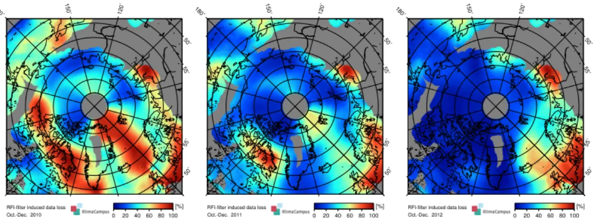
According to this RFI filter, strongly RFI affected regions are the region northeast of Greenland and parts of the Canadian Arctic Archipelago. Figure 2 shows the RFI induced data loss based on our RFI filter. The data loss in the figure is defined as the ratio between the number of RFI contaminated measurements and the number of total

10

measurements. As can be seen from Fig. 2, the RFI situation in the Arctic region has improved much since 2010.

2.1.3 Brightness temperature intensity

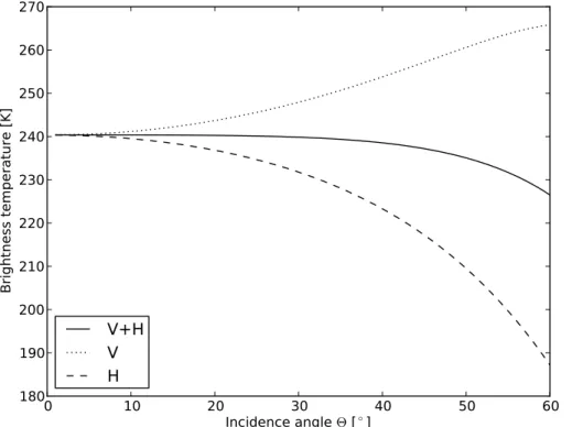
Over sea ice the first Stokes parameter (intensity) is almost independent of incidence angle in the incidence angle range of 0–40◦ (Fig. 3). The intensity is the average of

15

the horizontally and the vertically polarized brightness temperatures, i.e. it is equal to 0.5(TB_h+TB_v). The intensity is independent of both geometric and Faraday rotations and robust to instrumental and geophysical errors (Camps et al., 2005). We can avoid additional uncertainties caused by the transformation from the antenna reference frame to the Earth reference frame by using the intensity. Since each snapshot measures

ei-20

ther horizontally or vertically polarized brightness temperature, we use consecutive snapshots with an acquisition time di_fference of less than 2.5 s to calculate the inten-sity. The advantage of using near nadir view measurements is the smaller footprint associated with low incidence angles. Furthermore, by using the whole incidence an-gle range of 0–40◦ _{we get more than 100 brightness temperature measurements per}

25

(9)

TCD

7, 5735–5792, 2013

Title Page

Tables Figures

◭ ◮

Back Close

Full Screen / Esc

Discussion

P

a

per

|

D

iscussion

P

a

per

|

Discussion

P

a

per

|

Discuss

ion

P

a

per

|

neighbor algorithm and gridded into the National Snow and Ice Data Center (NSIDC) polar stereographic projection with a grid resolution of 12.5 km. We use this grid resolu-tion because other products that we use as auxiliary data in the retrieval are also given in this resolution. We call this product L3B brightness temperature. In the following we use TB to indicate the daily averaged brightness temperature intensity. The data have

5

been processed with about 24 h latency for both hemispheres and available since Jan-uary 2010. The L3B TBs are the basis of our sea ice thickness retrieval with Algorithm I and II and can be obtained from icdc.zmaw.de.

2.2 JRA-25 reanalysis data

For estimating the ice surface temperature, we extract the 2 m surface air temperature

10

and the 10 m wind velocity data from JRA-25 atmospheric reanalysis data and interpo-late them into the polar stereographic projection with 12.5 km grid resolution. JRA-25 reanalysis data provide various physical variables in 1.125◦ resolution every six hours. The data have been produced by the Japanese Meteorological Agency using the lat-est numerical analysis and prediction system. The data are available from 1979 to the

15

present (Onogi et al., 2007). Various studies have been carried out to compare the JRA-25, ERA40 and NCEP data sets. Good agreements were found between JRA-25 and ERA40 (Onogi et al., 2007).

2.3 Sea surface salinity climatology

The SSS information is needed to estimate the bulk ice salinity which is an input

param-20

eter of the radiation model of sea ice. There are global ocean salinity products derived from SMOS brightness temperatures. Ocean salinity is one of the two applications SMOS was originally designed for. However, SMOS-derived ocean salinity is not avail-able for the ice covered regions in the Arctic. Thus, we use a SSS climatology based on the outputs of an ocean-sea ice model. SSS weekly climatology is computed based on

25

(10)

TCD

7, 5735–5792, 2013

Title Page

Tables Figures

◭ ◮

Back Close

Full Screen / Esc

Discussion

P

a

per

|

D

iscussion

P

a

per

|

Discussion

P

a

per

|

Discuss

ion

P

a

per

|

Oceans’ circulations using the MIT general circulation ocean-sea ice coupled model (Marshall et al., 1997). The model is configured for the Atlantic Ocean north of 33◦S, including all Atlantic marginal seas and the Arctic Ocean up to the Bering Strait, and is integrated at the eddy-resolving resolution of approximately 4 km. The vertical resolu-tion of the model varies from 5 m in the upper ocean to 275 m in the deep (100 vertical

5

levels are used). Bottom topography is interpolated from the ETOPO2 database and ini-tial temperature and salinity conditions from a 8 km resolution integration of the same model (to achieve a good degree of spin-up), which in turn starts from the WOA09 climatology. The model is forced at the surface by fluxes of momentum, heat and fresh-water computed internally in the model with the help of the 6 hourly atmospheric state

10

from the ECMWF/ERA-Interim Reanalysis (Dee et al., 2011) and bulk formula. At the open northern (Bering Strait) and southern (33◦S) boundaries, the model is forced by a 1◦resolution global solution. The K-Profile Parameterisation (KPP) formulation is used for the parameterization of vertical mixing, with a background vertical viscosity coe_fficient of 1_×10−4_m2_{. The vertical di}

ffusion employed amounts to 1_×10−5_m2_s−1_.

15

Unresolved horizontal mixing uses a bi-harmonic diffusion/viscosity of 3_×109m4s−1. The overall good performance of the above model configuration (integrated at 8 km resolution), assessed through comparisons with in-situ measurements, can be found in Serra et al. (2010); Brath et al. (2010); Dmitrenko et al. (2012). We choose to use a model climatology and not Polar science center Hydrographic climatology (PHC) to

20

benefit from the dynamical oceanographic structures realistically resolved in the model, which leads to spatial and seasonal variability of SSS.

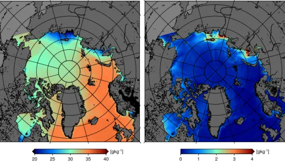
Figure 4 shows the mean and standard deviation of weekly SSS from October to April, based on 8 yr of daily model output. SSS in the Laptev Sea, parts of the Kara Sea, and the Baltic Sea is much lower than in the central Arctic due to the influence of

25

(11)

TCD

7, 5735–5792, 2013

Title Page

Tables Figures

◭ ◮

Back Close

Full Screen / Esc

Discussion

P

a

per

|

D

iscussion

P

a

per

|

Discussion

P

a

per

|

Discuss

ion

P

a

per

|

SSS should be considered in the retrieval when we calculate Arctic-wide ice thickness distributions.

2.4 MODIS ice thickness charts

MODIS ice thickness charts covering an area of 1500 km×1350 km over the Kara Sea and the eastern part of the Barents Sea have been calculated. The derivation

5

of the charts and their uncertainty estimation are described in detail in Maekynen et al. (2013). The total number of the charts is 120 and they cover two winters (November to April) in 2009–2011. The spatial resolution of the charts is 1 km and they show ice thickness from 0 to 99 cm. The external forcing data for solving the ice thickness from the surface heat balance equation come from a numerical weather prediction (NWP)

10

model HIRLAM (HIgh-Resolution Limited Area Model) (Kaellen, 1996; Unden, 2002). Only night-time MODIS data are employed. Thus, the uncertainties related to the ef-fects of solar shortwave radiation and surface albedo are excluded. For the cloud mask-ing of the MODIS data, in addition to the different cloud tests (Frey et al., 2008), also manual methods are used in order to improve the detection of thin clouds and ice fog.

15

The cloud masking is conducted with 10 km×10 km blocks to identify larger cloud-free areas and to reduce errors due to the MODIS sensor striping effect. In the ice thickness chart calculation an average snow thickness (h_s) vs. ice thickness (h_i) relationship is used. The thickness of the snow layer is assumed to be:

h_s=0 m for d_ice<0.05 m

20

hs=0.05×dice for 0.05 m≤dice<0.2 m

h_s=0.09_×d_ice for d_ice_≥0.2 m

This relationship is based on Doronin (1971) and the Soviet Union’s Sever expe-ditions data (NSIDC, 2004). The typical maximum reliable ice thickness (max 50 %

25

(12)

TCD

7, 5735–5792, 2013

Title Page

Tables Figures

◭ ◮

Back Close

Full Screen / Esc

Discussion

P

a

per

|

D

iscussion

P

a

per

|

Discussion

P

a

per

|

Discuss

ion

P

a

per

|

for the 15–30 cm thickness range, around 38 %. These figures are based on Monte Carlo method using estimated or guessed standard deviations and covariances of the input variables to the thickness retrieval. No in-situ data are available for the thickness accuracy estimation.

3 Sea ice thickness retrieval Algorithm II 5

Algorithm I is described in detail in Kaleschke et al. (2012), we will here introduce the retrieval Algorithm II. As in Algorithm I we use the daily mean brightness temperature intensity TB averaged over 0–40◦incidence angle range.

3.1 The sea ice radiation model

The basis of the SMOS ice thickness retrievals Algorithm I and II is the sea ice radiation

10

model adapted from Menashi et al. (1993). While for Algorithm I the radiation model is used to calculate the constant attenuation factorγ for a representativeT_ice andS_ice in the Arctic, in Algorithm II the model is used to calculate TB at variableT_ice andS_ice.

The sea ice radiation model consists of a plane ice layer bordered by the underlying sea water and air on the top. The model does not include a snow layer. The TB over

15

sea ice depends on the dielectric properties of the ice layer which are a function of brine volume (Vant et al., 1978). The brine volume is a function of Sice and Tice (Cox

and Weeks, 1983).

For a thin ice layer, the ice temperature gradient within the ice can be assumed to be linear (Maaß, 2013a). Assuming that the water under sea ice is at the freezing point, we

20

(13)

TCD

7, 5735–5792, 2013

Title Page

Tables Figures

◭ ◮

Back Close

Full Screen / Esc

Discussion

P

a

per

|

D

iscussion

P

a

per

|

Discussion

P

a

per

|

Discuss

ion

P

a

per

|

Sice is estimated using the empirical function of Ryvlin (1974)

Sice=Sw(1−SR)e−a

√ d_ice

+SRSw, (2)

whereS_wis the SSS,d_ice is the ice thickness (here in cm), S_Ris the salinity ratio of the bulk ice salinity at the end of the ice growth season and the SSS,ais the growth

5

rate coe_fficient which varies from 0.35 to 0.5. Ryvlin (1974) suggests to use 0.5 for a and 0.13 for S_R. However, Kovacs (1996) compared the Ryvlin empirical equation with observed data in the Arctic and suggests to use 0.175 forSRinstead of 0.13. In

our model we use 0.175 for S_R which seems to fit better to the observation data in the Arctic. Cox and Weeks (1983) give another empirical relationship betweenS_iceand

10

dice in the Central Arctic. The two empirical relationships have similar values for first

year ice and a water salinity of S_w=31 g kg−1 (Kovacs, 1996). The S_ice in Eq. (2) is a function of the underlying SSS, and can therefore be applied to regions outside the central Arctic where SSS is much lower.

The ice thickness retrieval with SMOS data is limited by the saturation of TB. We

15

consider TB to reach saturation if the change of TB with d_ice is less than 0.1 K per cm. Thus, TB of an ice layer with a Tice of −2◦C and a salinity of 8 g kg−1 reaches

its saturation for ice thicknesses of less than 20 cm, for example. This means that the maximal retrievable ice thicknessd_maxunder warmer conditions can be as low as a few centimeter. On the contrary, under cold conditions and a low ice salinity, which is typical

20

for coastal regions with river run-o_ff, L-band TB emanates from a thicker ice layer. TB reaches its saturation much more slowly andd_maxcan be as high as 1.5 m (Figs. 5 and 6). Therefore, SMOS ice thickness retrieval is more suitable for cold conditions and low ice salinity. If the ice temperature varies between₋5◦C and₋10◦C, which is typical for the Arctic in winter, the difference of retrieved ice thicknesses can be as high as 20 cm.

25

(14)

TCD

7, 5735–5792, 2013

Title Page

Tables Figures

◭ ◮

Back Close

Full Screen / Esc

Discussion

P

a

per

|

D

iscussion

P

a

per

|

Discussion

P

a

per

|

Discuss

ion

P

a

per

|

3.2 The thermodynamic model

In Algorithm II T_ice is estimated at each step from the d_ice and T_a. For this purpose thermal equilibrium is assumed at the surface of the ice layer and the heat fluxes are calculated with a thermodynamic model based on Maykut (1986). Although we neglect snow layer in the sea ice radiation model, we consider its thermal insulation e_ffect in the

5

thermodynamic model when we calculate theT_ice. It is shown in Maaß et al. (2013b) that the impact of a snow layer on the TB is partly caused by its insulation effect on the ice temperature. The insulation e_ffect of a snow layer increases with snow thickness. Linear temperature gradient profiles are assumed for the ice and snow layers in the model.

10

Under the assumption of thermal equilibrium, the incoming and outgoing heat fluxes compensate each other. During winter season, surface melting can be neglected. Therefore the heat balance at the surface of a slab ice layer with thicknessdice and

a layer of snow with thicknessh_son top can be described as

(1₋α)Fr−I0+FLin−FLout+Fs+Fe+Fc=0 (3)

15

whereF_r is the incoming shortwave radiation,α is the albedo of the snow/ice layer, I₀ is the part of the incoming shortwave radiation that is transmitted into the ice, F_Lin is the incoming longwave radiation,F_Lout is the outgoing longwave radiation, F_s is the sensitive heat flux,F_eis the latent heat flux, andF_c is the conductive heat flux.

20

The radiative and turbulent fluxes (1₋α)F_r−I0,FLin,FLout,Fe, andFs are calculated

as in Maykut (1986). For simplification we assume constant values for the cloud cover C, the relative humidityr, and the bulk transfer coefficients for sensible and latent heat flux C_s and C_e estimated from the reanalysis data. However, these parameters can be obtained from the auxiliary data that will be delivered with SMOS L1C data in the

25

(15)

TCD

7, 5735–5792, 2013

Title Page

Tables Figures

◭ ◮

Back Close

Full Screen / Esc

Discussion

P

a

per

|

D

iscussion

P

a

per

|

Discussion

P

a

per

|

Discuss

ion

P

a

per

|

The conductive heat fluxFcis given by

F_c= kiks

k_ih_s+k_sd_ice(Tw−Ts) (4)

wherek_sis the thermal conductivity of snow,T_wis the freezing point of sea water.k_s is set to 0.31 W m−1K−1according to Yu and Rothrock (1996). The thermal conductivity

5

of icek_ican be expressed as (Untersteiner, 1964)

k_i=2.034+0.13 Sice

T_ice−273, (5)

whereS_ice is in g kg−1andT_iceis in K.T_ice can be calculated with

Tice=0.5(Tsi+Tw), (6)

10

whereT_siis the snow-ice interface temperature calculated with

T_si=

T_s+ kihs

ksdiceTw

1₊ kihs

ksdice

. (7)

To calculate T_si we need to know k_i. However, k_i is in turn a function of T_ice. As

15

an approximation we first calculateki with 0.5(Ts+Tw) instead ofTice and use this ki

to calculate T_ice and T_si.T_s is estimated with leastsquare method for each d_ice under thermal equilibrium assumption.

3.3 Retrieval steps

As discussed in Sect. 3.1, the challenge of using variable T_ice and S_ice in the

Algo-20

(16)

TCD

7, 5735–5792, 2013

Title Page

Tables Figures

◭ ◮

Back Close

Full Screen / Esc

Discussion

P

a

per

|

D

iscussion

P

a

per

|

Discussion

P

a

per

|

Discuss

ion

P

a

per

|

forward model consisting of the radiation and thermodynamic model. Therefore, we approximated_ice by repeating the radiation and the thermodynamic model until a con-vergence point is found for the solution (Fig. 7). In this process, at each stepT_ice and Sice are calculated for the respectivedice approximation. The starting point of the

iter-ation is thed_ice retrieved with Algorithm I, which uses a constantT_ice of₋7◦C andS_ice

5

of 8 g kg−1. At each iteration step, we use d_ice,T_ice, andS_ice to calculate TB with the radiation model. The calculated TB is then compared with that observed by SMOS. To minimize the di_fference between the observed and the calculated TBs, the newd_iceis estimated with a linear approximation method. We define two stopping criteria for the iteration: a brightness temperature difference of less than 0.1 K, or an ice thickness

10

di_fference of less than 1 cm. The first criterion represents half of the optimal accuracy of daily averaged measurements. We apply the first criterion if the ice is thicker than 30 cm and otherwise the second criterion. Thed_maxis determined with the same crite-ria for the saturation of TB, i.e. that the TB change is less than 0.1 K per 1 cmd_ice. We define a saturation factor

15

S_TB=d_ice/d_max. (8)

If the saturation factor reaches 100 %, it indicates that the dmax can be considered

as the minimum ice thickness of the pixel.

4 Assessment of uncertainties 20

4.1 Systematic errors

In both algorithms we assume 100 % ice coverage for simplicity. TB over ice-sea water mixed areas can be described as

TB=TB_water_×(1₋IC)+TB_ice_×IC, (9)

(17)

TCD

7, 5735–5792, 2013

Title Page

Tables Figures

◭ ◮

Back Close

Full Screen / Esc

Discussion

P

a

per

|

D

iscussion

P

a

per

|

Discussion

P

a

per

|

Discuss

ion

P

a

per

|

where IC is the ice concentration, TB_waterand TB_ice are the TBs over sea water and ice, respectively.

SMOS TB_water shows a stable value of about 100.5 K with a standard deviation of about 1 K in the Arctic region. With this constant TB_water, we can calculate TB_ice using ice concentration charts from passive microwave radiometer data. During the winter

5

most of the ice covered area in the Arctic has IC higher than 90 % (Andersen et al., 2007). The passive microwave radiometer IC charts have an uncertainty of 5 % in the winter time (Andersen et al., 2007). At high concentrations, correcting the retrieved ice thickness with IC data set with an uncertainty of 5 % can cause higher errors than the 100 % ice coverage assumption. Therefore, we assume in the retrievals a 100 %

10

ice coverage. The possible underestimation of ice thickness due to this assumption is investigated with the simple semi-empirical function used in the Algorithm I. Figure 8 shows that the bias caused by this assumption increases exponentially with decreasing ice concentration. If we assume a SMOS TB of 220 K, the bias can be very high even for IC of more than 80 %. At lower brightness temperatures the bias caused by this

15

assumption is less than a few centimeters.

4.2 Sea ice thickness uncertainties

There are several factors that cause uncertainties in the sea ice thickness retrieval: the uncertainty of the SMOS TB, the uncertainties of the auxiliary data sets, and the assumptions made for the radiation and thermodynamic models.

20

For our purpose we average TB over the incidence angle range of 0–40◦. Due to the large amount of measurements in one day this can significantly reduce the uncer-tainty of TB by dividing standard deviation of TB with square root of the number of measurements during one day at each pixel. This uncertainty is less than 0.5 K in the Arctic except for the strongly RFI a_ffected regions. The uncertainties ofT_iceandS_ice

de-25

(18)

TCD

7, 5735–5792, 2013

Title Page

Tables Figures

◭ ◮

Back Close

Full Screen / Esc

Discussion

P

a

per

|

D

iscussion

P

a

per

|

Discussion

P

a

per

|

Discuss

ion

P

a

per

|

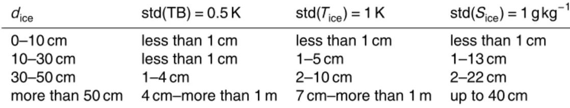
A first estimation of SMOS retrieved ice thickness uncertainty is made with Algorithm II based on the std(TB), std(T_ice) and std(S_ice). The std(TB) is calculated at each pixel with standard deviation of all available TB measurements divided by the sqrt(number of TB measurements) for each day. The std(Sice) is calculated based on the std(SSS)

chart (see Fig. 4) andd_ice. The estimation of std(T_ice) is rather di_fficult because it

de-5

pends not only on theT_abut also the assumptions made in the thermodynamic model. As a first approximation we assume 1 K for the std(T_ice) which is estimated with the vari-ations inT_a. More investigations should be conducted to better estimate the uncertainty inT_icein the future.

In Table 1 we show an example of estimated ice thickness uncertainties for

condi-10

tions whereT_ice varies from₋10◦C to₋2◦C andS_ice varies from 2 g kg−1 to 8 g kg−1. We assume a standard deviation of 0.5 K, 1 K, and 1 g kg−1 for TB, T_ice, and S_ice, re-spectively. The ice thickness uncertainty caused by std(TB) is rather small for thin ice less than 50 cm, and increases exponentially for thicker ice. The uncertainty caused by std(T_ice) is higher than that caused by std(TB) with an increasing trend with increasing

15

ice thickness.S_ice uncertainty has little impact on the ice thickness retrieval for saline ice with a S_ice of more than 5 g kg−1. However, for less saline ice, which is typical for example in the regions with river run-off, std(S_ice) has much more impact on the ice thickness uncertainty than the other two parameters ford_ice less than half a meter.

5 The effect of the subpixel-scale heterogeneity on the thickness retrieval 20

(Algorithm II* post-processing)

Natural sea ice is usually not a uniform layer of level ice with a plane geometry, as it was assumed in the emissivity model, but behaves fractally on a wide range of scales. Sea ice deformation patterns are often described using self-similar functions such as the lognormal distribution (Erlingsson, 1988; Key and McLaren, 1991; Tan et al., 2012).

25

(19)

evolu-TCD

7, 5735–5792, 2013

Title Page

Tables Figures

◭ ◮

Back Close

Full Screen / Esc

Discussion

P

a

per

|

D

iscussion

P

a

per

|

Discussion

P

a

per

|

Discuss

ion

P

a

per

|

tion of the thickness distribution (Thorndike, 1992; Godlovitch et al., 2012). A common feature of simulations and empirical observations is the exponential tail resulting from dynamic deformation processes. The inherent skewness of the thickness distribution results in a considerable underestimation of sea ice thickness when the retrieval model is based on a plane sea ice layer. In the following we use airborne sea ice thickness

5

measurements in order to parameterise the thickness distribution function and to in-vestigate the effect of the subpixel-scale heterogeneity on the thickness retrieval.

NASA’s Operation IceBridge (OIB) airborne campaigns obtained large scale profiles of sea ice thickness derived from a laser altimeter system (Kurtz et al., 2013). The footprint size of a single laser beam is about 1 m and the vertical accuracy is given

10

as 6.6 cm. The sea ice thickness is estimated from the freeboard by accounting for the snow thickness and assumptions about the densities of ice and snow. The snow thickness is retrieved using a snow-depth radar simultaneously. Here we use the OIB “quicklook” data as obtained from a NSIDC website.

We assume that the sea ice thickness follows a lognormal distribution

15

p(d_ice,µ,σ)₌ 1 d_iceσ√2πe

−(log(dice)−µ)

2

(2σ2) ₍₁₀₎

with the two parameters logmeanµand logsigmaσ. Furthermore, we assume a con-stant logsigma valueσto approximate the thickness distribution function with only one independent variable. To test this assumption we split the 2012 and 2013 OIB Arctic sea

20

ice thickness data in chunks of about 30 km length. We found that using constant val-uesσ=0.6_±0.1 rejects less than 15 % of the chunks tested with Kolmogorov-Smirnov statistics at a significance level of 95 %. The parameter σ increases with increasing length of the chunks and converges to about 0.7 for the maximal number of samples. The parameterσchanged only slightly from 0.692 to 0.695 while the mean thickness

25

(20)

TCD

7, 5735–5792, 2013

Title Page

Tables Figures

◭ ◮

Back Close

Full Screen / Esc

Discussion

P

a

per

|

D

iscussion

P

a

per

|

Discussion

P

a

per

|

Discuss

ion

P

a

per

|

value as large as 27.4 m which justifies the exponential tail of the distribution function. The e_ffect of the ice thickness distribution on TB is taken into account by the integration over the thickness range according to the superposition principle

TB∗₍_d

ice)=

max(Zdice)

0

TB(d_ice)g(d_ice)d d_ice (11)

5

with the thickness distribution function g(d_ice) and the brightness temperature of a single/plane-layer model TB(d_ice). The brightness temperature weighted with the thickness distribution TB∗ suggests a sensitivity to ice thicknesses larger than d_max. Hered_maxandd_iceboth refer to the single-layer thickness. The real mean thickness de-noted asHis strongly underestimated if the retrieval does not account for the thickness

10

distribution. The overall e_ffect can be explained as an apparently deeper penetration depth caused by the leading edge of the thickness distribution. The implementation of a radiative transfer model that includes this effect is straightforward but computationally expensive because of the integration. A post-processing look-up table for the single-layer model has been generated to estimate an approximate correction factor. This

15

method that converts the single-layer thicknessd_ice to the mean thickness H is called Algorithm II* hereinafter. Figure 10 shows that the involved correction factor increases with increasing salinity and temperature.

A main uncertainty is the shape of the thickness distribution and its parameterisation with a constantσ. This seems to be a reasonably good representation of the IceBridge

20

(21)

TCD

7, 5735–5792, 2013

Title Page

Tables Figures

◭ ◮

Back Close

Full Screen / Esc

Discussion

P

a

per

|

D

iscussion

P

a

per

|

Discussion

P

a

per

|

Discuss

ion

P

a

per

|

6 Comparison of ice thicknesses retrieved with Algorithms I, II, and II*

In this section, we analyse the time series of ice thicknesses retrieved from the Algo-rithm I, II, and II* at single grid points in the Laptev Sea and the Beaufort Sea (Point 1: 77.5◦N, 137.5◦E, Point 2: 71.0◦N, 165.0◦W, Point 3: 74.5◦N, 127.0◦E). The time series begin on 15 October 2011. The time series of ice thickness extracted from two

5

different sea ice assimilation systems are included for comparison. In addition, we show time series of SMOS TB together with ice concentration and derived snow/ice surface temperature.

One of the assimilation systems is the TOPAZ system. TOPAZ is an advanced data assimilation system, using the Ocean model HYbrid Coordinate Ocean Model

(HY-10

COM) and Elastic-Viscous-Plastic (EVP) ice rheology (Bertino and Lisæter, 2008). TOPAZ has a resolution between 18 and 36 km with 22 isopycnal layers. The as-similated observations are satellite-observed Sea Level Anomaly (SLA), Sea Surface Temperature (SST), sea ice concentrations from AMSR-E, sea ice drift products from CERSAT, and Coriolis in-situ temperature and salinity profiles. The TOPAZ system has

15

been in operation since 1 January 2003. The major outcomes in terms of products are weekly issued short term forecasts.

The other assimilation system is the Panarctic Ice Ocean Modeling and Assimilation System (PIOMAS) (Zhang and Rothrock, 2003). It is based on a coupled ocean-ice model forced with National Centers for Environmental Prediction Atmospheric

Reanaly-20

sis data. PIOMAS assimilates satellite-observed sea ice concentration and sea surface temperature data.

At Point 1, which is located in the north of the Laptev Sea, in the first 30 days Algo-rithm I and II show very similard_ice ranging from 0 m to about 0.3 m (Fig. 11). The TB increases from about 100 K to about 230 K. In this TB range,d_ice is the dominant factor

25

(22)

TCD

7, 5735–5792, 2013

Title Page

Tables Figures

◭ ◮

Back Close

Full Screen / Esc

Discussion

P

a

per

|

D

iscussion

P

a

per

|

Discussion

P

a

per

|

Discuss

ion

P

a

per

|

little variability with a mean value of 237.4 K and a standard deviation of 1.9 K. In this period,d_ice from Algorithm I shows a stable value around 0.35 m with a standard devi-ation of 3 cm, which results from the constant parameters assumed in Algorithm I. On the contrary,dice from Algorithm II shows an average value of 0.48 m with a standard

deviation of 11 cm. The strong variability ind_ice is mainly caused byT_ice. A correlation

5

coefficientR of−0.7 can be found betweenT_iceandd_ice. In the total time period of 200 days, the d_ice from Algorithm II is on average 10 cm thicker than that from Algorithm I. The ice thickness corrected with the thickness distribution function (Algorithm II*) is about two times that of Algorithm II.

Simulated ice thicknesses from TOPAZ and PIOMAS show continuous ice growth

10

during the time period, however, with more than half a meter span between them (shaded area in the upper panel of Fig. 11). The ice thicknesses retrieved with Algo-rithm II* correspond well with those from TOPAZ and PIOMAS in the first three months. However, from March to April TOPAZ and PIOMAS show further growth in the ice thick-ness, whereas SMOS shows rather constant or decreasing trends. The decreasing

15

trend ind_ice corresponds to the decreasingd_maxcaused by the increasingT_s.

Point 2 is located in the Beaufort Sea, near Barrow. The first sea ice occurrence happens in mid-November, one month later than at Point 1. A few days after the first occurrence of sea ice, the ice concentration rapidly reaches nearly 100 % (Fig. 12). In the following 80 days, theT_s decreases from about 270 K to 240 K,d_ice retrieved with

20

Algorithm II* increases from a few centimeters to more than 1.5 m. In this period, the ice thickness growth from SMOS Algorithm II* agrees well with that simulated by TOPAZ and PIOMAS. Just as at point 1, after the three months freeze-up period the SMOS retrievedd_icereaches its maximum with a decreasing trend in April, which corresponds to the increasingT_s.

25

(23)

TCD

7, 5735–5792, 2013

Title Page

Tables Figures

◭ ◮

Back Close

Full Screen / Esc

Discussion

P

a

per

|

D

iscussion

P

a

per

|

Discussion

P

a

per

|

Discuss

ion

P

a

per

|

wind conditions force the riverine water northwards and result in a stronger density stratification in the eastern Laptev sea during winter. Cyclonic atmospheric circulation deflects the freshwater plume of the Lena river eastward towards the East Siberian Sea, thus causing higher salinity in the eastern Laptev Sea and the area around the West New Siberian (WNS) polynya.

5

The strong variability of ice thicknesses in SMOS and PIOMAS shows good correla-tion (Fig. 13). The decrease and increase of ice thicknesses in SMOS and in the model outputs are very likely caused by the drift of thick ice due to wind forcing and thin ice formation in the polynya areas. From March to April, there is a large discrepancy be-tween the model outputs and the SMOS-derived ice thickness. While PIOMAS shows

10

an ice thickness of more than 2 m in April, SMOS-derived ice thickness is less than half a meter.

Sea ice thickness measurements were carried out in this area during helicopter-borne ice thickness surveys performed in the Laptev Sea during the Transdrift (TD) XX campaign in April 2012. The helicopter-borne ice thickness measurements were made

15

with an electromagnetic (EM)-Bird that utilizes the contrast of electrical conductivity between sea water and ice to determine the distance to the ice-water interface (Haas et al., 2009). An additional laser altimeter yields the distance to the uppermost reflect-ing surface. Hence, the obtained ice thickness is the ice- plus snow thickness from the di_fference between the laser range and the EM-derived distance. The accuracy over

20

level sea ice is in the order of 10 cm (Pfa_ffling et al., 2007). Uncertainties in the ice thick-ness measurements may arise from the assumption that sea ice is a non-conductive medium. Over thin ice, this assumption may be invalid because the conductivity of saline young ice can be significantly higher than that of older first-year or multi-year ice. This can lead to an underestimation of ice thickness.

25

(24)

TCD

7, 5735–5792, 2013

Title Page

Tables Figures

◭ ◮

Back Close

Full Screen / Esc

Discussion

P

a

per

|

D

iscussion

P

a

per

|

Discussion

P

a

per

|

Discuss

ion

P

a

per

|

the flight track. Therefore, we use the EM-Bird measurements to validate the SMOS derived ice thickness. During the flights, the EM-Bird recorded a total of 46386 mea-surements with a mean value of 43 cm and a standard deviation of 33 cm. This agrees well with the 31 cm ice thickness from SMOS Algorithm II*, considering that the EM-Bird derived ice thickness is the sum of the thicknesses of the ice layer and the snow

5

layer on top of it. The comparison shows that in the polynya area SMOS estimates the ice thickness better than TOPAZ or PIOMAS.

After the time series comparison at single points, we compare the daily ice thickness distribution from the three algorithms in the Arctic on 1 February 2013. As can be seen in Fig. 14, the mean ice thickness considerably increases from Algorithm I to Algorithm

10

II*. In the central Arctic covered with thick multi-year ice, the TB reaches its saturation. Therefore, none of the algorithms can deliver reliable ice thickness information in the thick multi-year ice area. If we consider only the pixels where TB has not reached its saturation, ice thickness from Algorithm II* is on average 0.82 m, which is about 40 cm thicker than that from Algorithm II and 55 cm thicker than that from Algorithm I.

15

However, the increase of ice thickness varies from region to region, depending on SSS and weather conditions. For example, in the Laptev Sea where the SSS is much lower than that in the central Arctic, the di_fference between Algorithm II and Algorithm I is as large as half a meter. On the contrary, in parts of the Kara Sea and north of the Barents Sea little change can be observed between Algorithm I and II. The increase

20

of ice thickness in Algorithm II compared to Algorithm I is caused by the deviation of estimatedT_iceandS_icefrom the constant values assumed in Algorithm I. To investigate the contribution ofTice andSice in the thickness retrieval separately we carried out two

tests with the data of 1 February 2013. In the first testS_iceis assumed to be 8 g kg−1_as

in Algorithm I and we vary onlyT_ice. In the second testT_iceis assumed to be−7◦C as in

25

(25)

TCD

7, 5735–5792, 2013

Title Page

Tables Figures

◭ ◮

Back Close

Full Screen / Esc

Discussion

P

a

per

|

D

iscussion

P

a

per

|

Discussion

P

a

per

|

Discuss

ion

P

a

per

|

thickness change caused bySicefrom Test 2 is on average 3 cm. However, up to 20 cm

and 60 cm di_fference can be found in the Laptev Sea and in the Baltic Sea.

The comparisons show that Algorithm II* has a considerably better agreement with the model outputs and the EM-Bird validation data than Algorithm I and II. Taking into account the variability of ice temperature and ice salinity delivers better information

5

about the Arctic-wide ice thickness distribution. Therefore, we use Algorithm II* to re-trieve ice thickness in our operational data processing.

7 Ice thickness growth and distribution as seen by SMOS during the freeze-up period

SMOS-derived ice thickness shows continuous growth and expansion of first year ice

10

in the Arctic during the freeze-up period. Figure 15 shows the monthly mean sea ice thickness from October 2012 to March 2013 retrieved with Algorithm II*. From October to November, thin first-year ice extends to most areas of the East Siberian Sea, the Laptev Sea, and the Beaufort Sea. In addition to the area expansion, also an increase of ice thickness due to the thermodynamic growth can be observed. In December,

first-15

year ice reaches a thickness of more than 1 m in the Laptev Sea and the Beaufort Sea. In March 2013 large areas of thin ice with a thickness less than 40 cm are observed in the Beaufort Sea which is caused by the opening of leads and polynyas in this period.

8 Comparison of SMOS and MODIS ice thickness charts in the Kara Sea

8.1 Sea ice thickness derived from MODIS data 20

(26)

TCD

7, 5735–5792, 2013

Title Page

Tables Figures

◭ ◮

Back Close

Full Screen / Esc

Discussion

P

a

per

|

D

iscussion

P

a

per

|

Discussion

P

a

per

|

Discuss

ion

P

a

per

|

compare SMOS and MODIS ice thicknesses, we reduce the 1 km spatial resolution of the MODIS thickness charts to the NSIDC grid resolution of 12.5 km by spatial averag-ing.

We first compare ice thickness distributions from SMOS and MODIS for two selected days (26 December 2010 and 2 February 2011), on which a su_fficient amount of pixels

5

with valid MODIS data is available. After that, we collect all pixels with valid MODIS data from 30 days during the two winter seasons 2009–2010 and 2010–2011 and carry out a pixel to pixel comparison. The 30 days are selected manually. MODIS ice charts with strong cloud limitation are excluded. Similarly to Algorithm I and II, the MODIS sea ice thickness retrieval assumes a plane ice layer. Therefore, by spatial averaging of MODIS

10

data to a grid resolution of 12.5 km we use the modal mean of the MODIS ice thickness instead of the arithmetic mean. For the comparison we use the plane layer SMOS ice thickness, not the inhomogeneous mean ice thickness of Algorithm II*.

8.2 Daily comparison

Figure 16 shows the averaged MODIS ice thickness in a 12.5 km grid resolution, the

15

SMOS ice thicknesses retrieved from Algorithm I and II, and the histogram of the three ice thickness data in the Kara Sea on 26 December 2010. Ice concentration from the same day (Fig. 17) shows near 100 % ice coverage in the ice-covered area except for the marginal ice zone. We use here the ice concentration maps derived from SSM/I with the ARTIST Sea Ice (ASI) algorithm. Both SMOS and MODIS show similar patterns

20

of thin and thick ice distributions, whereas SMOS ice thickness from Algorithm I is considerably lower than the other two in the thicker ice range. Surface air temperature over the ice covered area varies from ₋30 to ₋20◦C (Fig. 17), providing favorable conditions for both SMOS and MODIS ice thickness retrievals (Kaleschke et al., 2010; Yu and Rothrock, 1996).

25

(27)

tem-TCD

7, 5735–5792, 2013

Title Page

Tables Figures

◭ ◮

Back Close

Full Screen / Esc

Discussion

P

a

per

|

D

iscussion

P

a

per

|

Discussion

P

a

per

|

Discuss

ion

P

a

per

|

perature as a boundary condition. The SMOS-derived snow surface temperature is in good agreement with that from the MODIS snow/ice surface temperature product (Hall et al., 2004) (Fig. 17). The mean surface temperatures from MODIS and SMOS are both 247 K, and the root mean square deviation (RMSD) is 4 K. Discrepancies can be seen in the marginal ice zone and in the Ob estuary where the low salinities are not

5

well represented by the ocean model. In the marginal ice zone with lower ice concen-trations, SMOS strongly underestimates ice thickness, which leads to too warm surface temperatures. The surface temperature is used in SMOS Algorithm II to calculate the bulk ice temperature, which is a variable parameter in the radiation model to calculate the emissivity of an ice layer.

10

In total there are 4167 pixels in 12.5 km grids with valid MODIS ice thicknesses. For these pixels MODIS has a mean thickness of 44 cm, whereas SMOS has an average of 32 cm and 47 cm from Algorithm I and II, respectively. The correlation coefficientR and RMSD between the SMOS Algorithm II and MODIS are 0.60 and 20 cm, whereas for SMOS Algorithm I and MODIS they are 0.57 and 23 cm, respectively. If we only

con-15

sider the 2679 pixels with a MODIS ice thickness less than 50 cm, mean ice thicknesses of SMOS Algorithm I, SMOS Algorithm II and MODIS are 29 cm, 40 cm, and 29 cm re-spectively. That means in the thin ice range Algorithm II overestimates ice thickness compared to MODIS. The bulk ice temperature derived from the surface temperature in Algorithm II is on average 263.6 K, which is 2.5 K lower than that assumed in SMOS

20

Algorithm I. This can partly explain the ice thickness di_fference between Algorithm I and II. The SMOS-derived ice thickness decreases with increasing ice temperature at the ice temperature as low as₋10◦C (Maaß, 2013a).

Similar results can be derived from another comparison on 2 February 2011 (see Figs. 18 and 19). On this day, large areas of thin ice can be observed from SMOS and

25

(28)

TCD

7, 5735–5792, 2013

Title Page

Tables Figures

◭ ◮

Back Close

Full Screen / Esc

Discussion

P

a

per

|

D

iscussion

P

a

per

|

Discussion

P

a

per

|

Discuss

ion

P

a

per

|

is normally higher than 90 %, except for the marginal ice zone. Like on 26 Decem-ber 2010, surface air temperature in the Kara Sea is as low as ₋30◦C. In total 4016 pixels have valid MODIS data. The mean ice thickness of SMOS Algorithm I, SMOS Algorithm II, and MODIS for the pixels are 33 cm, 50 cm, and 47 cm, respectively. The correlation coe_fficient and RMSD between the SMOS Algorithm II and MODIS are 0.61

5

and 21 cm, whereas between SMOS Algorithm I and MODIS they are 0.59 and 26 cm, respectively. The mean surface tempertures from MODIS and SMOS are 246 K and 245 K, with a RMSD of 4 K.

8.3 Comparison with 30 days data from the two winter seasons

In total 33 and 87 days of MODIS validation data are available for the winter seasons

10

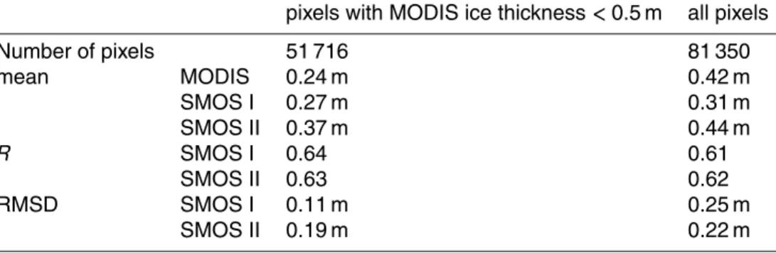
of 2009–2010 and 2010–2011. However, many of them have only small areas with usable MODIS data. Therefore, we selected out 30 days on that the data are not badly affected by cloud coverage. Altogether 81350 pixels are available in 12.5 km resolution. The histogram of the ice thicknesses (Fig. 20) shows better agreement between SMOS Algorithm II and MODIS than between SMOS Algorithm I and MODIS for these pixels.

15

The mean ice thicknesses derived from SMOS Algorithm II and MODIS are of the same order, 44 cm and 42 cm, respectively, whereas SMOS Algorithm I shows on average 31 cm. If we restrict the comparison to the pixels with MODIS ice thicknesses less than 50 cm, the mean ice thickness from SMOS Algorithm II is about 13 cm higher than the MODIS mean value (see Table 2).

20

9 Conclusions

In this study we developed a new SMOS sea ice thickness retrieval algorithm (de-noted as Algorithm II) in which we take into account variations of ice temperatureT_ice and salinityS_ice.T_ice andS_ice are estimated during the ice thickness retrieval from the surface air temperature T_a of atmospheric reanalysis data and a model-based SSS