Observation of horizontal winds in the middle-atmosphere between 30° S and 55° N during the northern winter 2009–2010

www.atmos-chem-phys.net/13/6049/2013/ doi:10.5194/acp-13-6049-2013

© Author(s) 2013. CC Attribution 3.0 License.

Atmospheric

Chemistry

and Physics

Geoscientiic

Geoscientiic

Geoscientiic

Geoscientiic

Observation of horizontal winds in the middle-atmosphere between

30

◦

_{S and 55}

◦

_{N during the northern winter 2009–2010}

P. Baron1, D. P. Murtagh2, J. Urban2, H. Sagawa1, S. Ochiai1, Y. Kasai1,6, K. Kikuchi1, F. Khosrawi3, H. K¨ornich4, S. Mizobuchi5, K. Sagi2, and M. Yasui1

1_{National Institute of Information and Communications Technology, 4-2-1 Nukui-kitamachi, Koganei, Tokyo 184-8795, Japan} 2_{Department of Earth and Space Science, Chalmers University of Technology, 41296 G¨oteborg, Sweden}

3_{Department of Meteorology Stockholm University, 10691 Stockholm, Sweden} 4_{SMHI, Folkborgsv¨agen 17, 60176 Norrk¨oping, Sweden}

5_{Japan Aerospace Exploration Agency, Tsukuba, 305-8505 Japan}

6_{Tokyo Institute of Technology, 4259 Nagatsuta-cho, Midori-ku, Yokohama, Kanagawa 226-8503, Japan}

Correspondence to:P. Baron (baron@nict.go.jp)

Received: 17 October 2012 – Published in Atmos. Chem. Phys. Discuss.: 17 December 2012 Revised: 17 May 2013 – Accepted: 17 May 2013 – Published: 25 June 2013

Abstract.Although the links between stratospheric dynam-ics, climate and weather have been demonstrated, direct observations of stratospheric winds are lacking, in partic-ular at altitudes above 30 km. We report observations of winds between 8 and 0.01 hPa (∼_{35–80 km) from October} 2009 to April 2010 by the Superconducting Submillimeter-Wave Limb-Emission Sounder (SMILES) on the Interna-tional Space Station. The altitude range covers the region between 35–60 km where previous space-borne wind instru-ments show a lack of sensitivity. Both zonal and meridional wind components were obtained, though not simultaneously, in the latitude range from 30◦S to 55◦N and with a single profile precision of 7–9 m s−1between 8 and 0.6 hPa and bet-ter than 20 m s−1at altitudes above. The vertical resolution is 5–7 km except in the upper part of the retrieval range (10 km at 0.01 hPa). In the region between 1–0.05 hPa, an absolute value of the mean difference <2 m s−1 is found between SMILES profiles retrieved from different spectroscopic lines and instrumental settings. Good agreement (absolute value of the mean difference of ∼_{2 m s}−1_{) is also found with} the European Centre for Medium-Range Weather Forecasts (ECMWF) analysis in most of the stratosphere except for the zonal winds over the equator (difference>5 m s−1_{). In}

the mesosphere, SMILES and ECMWF zonal winds exhibit large differences (>20 m s−1_{), especially in the tropics. We}

illustrate our results by showing daily and monthly zonal wind variations, namely the semi-annual oscillation in the

tropics and reversals of the flow direction between 50–55◦N during sudden stratospheric warmings. The daily comparison with ECMWF winds reveals that in the beginning of Febru-ary, a significantly stronger zonal westward flow is mea-sured in the tropics at 2 hPa compared to the flow computed in the analysis (difference of∼_{20 m s}−1_{). The results show} that the comparison between SMILES and ECMWF winds is not only relevant for the quality assessment of the new SMILES winds, but it also provides insights on the quality of the ECMWF winds themselves. Although the instrument was not specifically designed for measuring winds, the re-sults demonstrate that space-borne sub-mm wave radiome-ters have the potential to provide good quality data for im-proving the stratospheric winds in atmospheric models.

1 Introduction

Sigmond et al., 2008; Marshall and Scaife, 2009; Wang and Chen, 2010). In addition, stratospheric winds describe and affect vertically propagating atmospheric waves that con-trol the transport circulation in the stratosphere and meso-sphere (Holton and Alexander, 2000).

In meteorological analyses and reanalyses, unobserved variables are constrained by observed ones through the use of balance relationships. The application of a mass-wind balance (Derber and Bouttier, 1999) leads to a state where the large number of temperature soundings provide a strong constraint on the balanced wind component, i.e. approxi-mately the geostrophic wind. However, it is difficult to de-rive the larger scale wind fields using the geostrophic as-sumption in the tropics because the Coriolis parameter van-ishes at the equator and the solutions become numerically unstable (Hamilton, 1998; ˇZagar et al., 2004; Polavarapu et al., 2005). For instance, significant differences are seen be-tween wind climatologies derived from mass balance (Flem-ing et al., 1990; Randel et al., 2004). A further compli-cation in the middle atmosphere is that the small errors from the lower atmosphere propagate vertically and amplify strongly in the upper stratosphere and mesosphere (Nezlin et al., 2009; Alexander et al., 2010). Thus, in order to con-strain middle atmospheric winds in meteorological analyses, global wind observations in the middle atmosphere are es-sential. Lahoz et al. (2005) have shown that wind observa-tions on a global scale with a precision of 5 m s−1between 25 and 40 km would provide significant improvements of zonal-wind analyses especially in the tropical middle and upper stratosphere (50–1 hPa).

In spite of the importance of middle atmospheric obser-vations, wind measurements assimilated in the models are mostly limited to the troposphere. In the mesosphere, winds are measured using optical techniques from satellites (Shep-herd et al., 1993; Hays et al., 1993; Killeen et al., 1999; Swinbank and Ortland, 2003; Niciejewski et al., 2006) and by ground-based radar systems such as European Incoherent SCATter (EISCAT) (Alcayd´e and Fontanari, 1986) and vari-ous meteor radars (Maekawa et al., 1993; Jacobi et al., 2009). Wu et al. (2008) have used the microwave oxygen line at 118 GHz measured by the Microwave Limb Sounder (MLS) to derive line-of-sight winds in the mesosphere (70–92 km). The authors suggested that winds can be derived down to 40 km by using emission lines from other molecules, but no results have been shown yet. Stratospheric winds have been measured from the ground using active and passive tech-niques (Hildebrand et al., 2012; R¨ufenacht et al., 2012) and from space by the High Resolution Doppler Imager (HRDI) on UARS covering 10–35 km and 60◦S–60◦N, using the molecular oxygen A- and B-bands (Ortland et al., 1996).

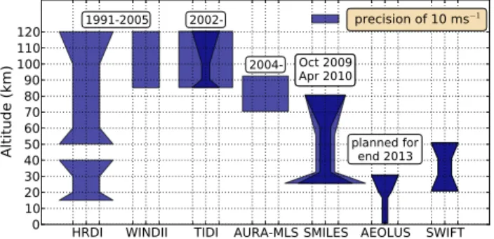
Figure 1 summarises previous and planned wind measur-ing instruments from spaceborne platforms. A gap in the cov-erage of high quality winds (<5 m s−1error) between 30 and 60 km clearly exists. The ESA Atmospheric Dynamics Mis-sion on the Aeolus satellite is planned for 2013–2014

(Stof-HRDI WINDII TIDI AURA-MLS SMILES AEOLUS SWIFT 0

10 20 30 4050 60 70 80 90 100 110 120

Altitude (km)

precision of 10 ms−1

1991-2005

2002-2004- Oct 2009_{Apr 2010}Oct 2009 Apr 2010

planned for end 2013

Fig. 1. The height coverage and estimated precision of past, current and future wind measuring instruments: reported validated preci-sions are in blue and theoretical values are in darker blue. HRDI (Ortland et al., 1996) and WINDII (Shepherd et al., 1993) were on the UARS satellite and operated from September 1991–June 2005, TIDI (Niciejewski et al., 2006) operates on the TIMED satel-lite from 2002-present, AURA-MLS (Wu et al., 2008) operates on the AURA satellite from July 2004–present (note that wind is not a standard product), SMILES operated on the ISS from September 2009–April 2010, Aeolus is ESA mission (Stoffelen et al., 2005) planned for 2013 and SWIFT (McDade et al., 2001) is under study in Canada.

felen et al., 2005) for measuring winds in the troposphere and lower stratosphere using a UV lidar. For middle-stratospheric winds, the Stratospheric Wind Interferometer For Transport studies (SWIFT) instrument was planned by the Space Cana-dian Agency for 2010 (McDade et al., 2001), but has an un-clear future at the time of writing. The target of SWIFT is to measure the thermal emission from O3lines at 8 µm in order

to provide winds on a near global scale between 15–50 km with the best accuracy of 3–5 m s−1 _{between 20–40 km and}

a vertical resolution of 2 km.

Here we report the first spaceborne observations of winds in the altitude gap 30–60 km using the Superconducting Submillimeter-Wave Limb-Emission Sounder (SMILES) on-board the Japanese Experiment Module (JEM) of the Interna-tional Space Station (ISS) (Kikuchi et al., 2010; Ochiai et al., 2012b). The instrument has been conceived for measuring trace gas profiles and was launched in September 2009. Al-though SMILES was not designed for this purpose, we have exploited its high frequency resolution and high signal-to-noise ratio to derive the small Doppler shifts in the atmo-spheric spectra and thereby line-of-sight wind velocities. Be-cause of the ISS rotation during an orbit, components near the meridional and the zonal directions are retrieved between 30◦_S–55◦_{N. As shown in this analysis, the wind} informa-tion is derived from 8–0.01 hPa (∼_{35–80 km) with a} preci-sion better than 10 m s−1at altitudes between 6 and 0.5 hPa and better than 20 m s−1at altitudes above.

SMILES measurements with the operational wind analysis by the European Centre for Medium-Range Weather Fore-casts (ECMWF). At mid-latitudes in the middle-stratosphere, ECMWF winds are expected to provide a wind represen-tation with an error smaller than that of a SMILES single retrieval and, thus, to provide a good dataset to check the SMILES wind quality. On the other hand, ECMWF results are uncertain in the middle and upper stratosphere of the trop-ical regions (Baldwin and Gray, 2005). The spread of a per-turbed Ensemble of Data Assimilations (EDA) at ECMWF indicates a precision of about 3 m s−1for the tropical middle-stratospheric zonal winds (Isaksen et al., 2010). The EDA method does not give information about the accuracy, and be-cause of the lack of other stratospheric wind measurements, SMILES data offer a unique opportunity to estimate it.

In Sect. 2, we briefly describe the measurement method. The theoretical precision (random errors) and accuracy (sys-tematic errors) are estimated from a sensitivity study. Sec-tion 3 assesses the quality of the SMILES data by check-ing the internal consistency of the different SMILES prod-ucts and their mean differences with the ECMWF winds. In Sect. 4, the results are illustrated with monthly global maps and the daily variation of the zonal-winds. Both the measured Semi-Annual Oscillations (SAO) of the zonal-wind above the Equator, and the zonal-wind reversals between 50–55◦N during Arctic Sudden Stratospheric Warming (SSW) events are discussed and are compared with the ECMWF analysis. Finally, we summarise our results and give conclusions as well as discuss ongoing work for improving the SMILES winds.

2 SMILES observations

2.1 Measurement method

SMILES was attached to the ISS in Sept 2009 and functioned for 7 months until April 2010. It observed the Earth’s limb, scanning from−_{7 to 100 km in 53 s, providing 1600 spectral} radiance profiles per day. Using Superconductor-Insulator-Superconductor (SIS) detectors cooled at 4 K, it provided high quality spectra allowing constituent profiles of many species such as ozone (O3) and hydrogen chloride (HCl) to

be derived (Kasai et al., 2006; Takahashi et al., 2010; Khos-ravi et al., 2012; Kasai et al., 2013). SMILES observed spec-tral lines from the atmospheric limb in three frequency bands, named A (624.3–625.5 GHz), B (625.1–626.3 GHz) and C (649.1–650.3 GHz) but only two are measured simultane-ously. Two acousto-optical spectrometers (1 and AOS-2) with similar specifications are used. Frequency calibra-tion and stability are ensured using an ultra-stable oscillator and frequent comb calibration of the AOS (Mizobuchi et al., 2012b). Inherent in the spectra is information on the Doppler shift caused by the ISS (∼_{4 km s}−1_{along the line of sight) as} well as atmospheric motion. The broadening of the spectral

lines into several spectral channels provides enough sensitiv-ity to detect the small frequency shift induced by the winds (e.g. a 50 m s−1_{line-of-sight wind induces a shift of 100 kHz}

which has to be compared to the spectrometer spectral res-olution of 1.2 MHz and to the full-width-half-maximum of the spectral line that decreases from∼_{50 MHz at 10 hPa to} ∼_{1 MHz at 0.2 hPa). For deriving wind, the two strongest} spectral lines have been used separately. One is an emission line of O3at 625.371 GHz common to bands A and B, and

the second one is a H35Cl triplet at 625.92 GHz (band B). Hence, three wind profiles are independently retrieved, two from the O3 line in bands A and B, and one from the HCl

triplet in band B. The wind retrieval algorithm is similar to the one presented in Baron et al. (2011) for the temperature and trace gas profiles retrieval (see Appendix for more de-tails). Profiles of geophysical parameters are retrieved from the inversion of the set of spectra that are measured during a single vertical scan of the atmospheric limb. To simplify and speed-up the retrieval calculations, the same line-of-sight ve-locity is removed from all spectra composing a vertical scan. The velocity which changes from one scan to another, is cho-sen at the middle of the scan. After the retrieval calculation, the derived wind profile is corrected from the altitude varia-tion of the line-of-sight velocity (∼_{0.8 m s}−1_km−1_).

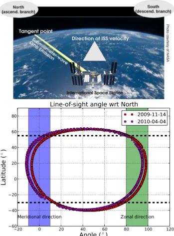
As seen in Fig. 2, because of the geometry of the instru-ment field-of-view in relation to the ISS orbit, the line-of-sight winds during the ascending (descending) portion of an orbit are almost in meridional (zonal) direction. Figure 3 shows single line-of-sight wind retrievals at 36 km on 2 and 26 January for both ascending and descending portions of the orbits. Between∼30◦_{S to∼55}◦_{N, the line-of-sight} direc-tion do not deviate by more than 10◦ _{from the exact zonal} or meridional directions. The full latitude range of observa-tions is between 38◦S and 65◦N but on the borders, the line-of-sight rotates quickly and deviates from the meridional or zonal direction. Another characteristic of the observations is, as the result of the 2 months periodic local-time precession of the ISS, semidiurnal and diurnal variations of mesospheric winds such as those induced by tides are captured in the ob-servations.

2.2 Theoretical estimation of the retrieval errors

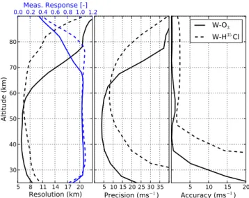
Figure 4 (left panel) shows the vertical resolution of the re-trieved wind profiles and the measurement responses, i.e., the sum of the averaging kernel rows (Merino et al., 2002) that indicate the altitudes of good measurement sensitiv-ity. Good sensitivity (defined as where the measurement re-sponse ranges from 0.9 to 1.1) is found from 25 to 70 km (20–0.05 hPa) and from 25 to 80 km (20–0.01 hPa) for the O3and HCl line retrievals, respectively. In the mesosphere,

the steep decrease of the O3concentration is responsible of

the loss of the retrieval sensitivity from the O3 line and the

20 0 20 40 60 80 100 120

Angle (◦₎ 60

40 20 0 20 40 60 80

La

ti

tu

de

(

◦ )

Meridional direction Zonal direction

Line-of-sight angle wrt North

2009-11-14 2010-04-04

Fig. 2.Upper panel: Representation of the limb observation

ge-ometry (adapted from http://smiles.nict.go.jp/pub/about/principles. html). The ISS orbit inclination is 51.6◦with respect to the equator and the SMILES line-of-sight is tilted by 45◦on the left side of the forward direction. The tangent point is at a distance of∼2000 km from the ISS. North (South) direction is indicated for the ascending (descending) orbit branch. Lower panel: latitudinal variation of the line-of-sight angle with respect to the North direction on 14 Novem-ber 2009 (red circles) and on 4 April 2010 (magenta circles). The blue (green) region indicates the region where the line-of-sight is between±10◦ about the meridional (zonal) direction. The thick dashed horizontal lines indicate the latitude range between 30◦S and 55◦N.

the upper-stratosphere and lower-mesosphere, and the HCl spectrum is composed of three relatively strong spectral lines within a narrow range of 30 MHz. According to the vertical resolution of the retrieved profiles, the best information is obtained from the O3line below 60 km (0.2 hPa), and from

the HCl lines at altitudes above. The vertical resolution of the composite retrieved profile is 5–7 km up to 70 km and in-creases to 10 km at 80 km. Since the wind information comes from a layer of 5 to 10 km thickness around the of-sight tangent point, the horizontal resolution along the line-of-sight is between 500 and 700 km.

The theoretical precision and accuracy for a single profile retrieval are shown in the central and right panels of Fig. 4, respectively. The methodology and the assumptions of the ror analysis are given in Baron et al. (2011), except for the er-rors on the calibration parameters which include a correction for a nonlinearity in the receiver which was not applied in the previous analysis (Ochiai et al., 2012a). An error of 20 % is assumed on the nonlinear parameters. The retrieval precision is limited by the measurement noise and to a lesser extent by the uncertainties in the O3and HCl abundances. The

theoret-ical precision is 4–10 m s−1between 35 and 60 km (O3line

retrieval) and <20 m s−1 between 60 and 80 km (HCl line retrieval). The accuracy of the retrieval at lower altitudes is set by systematic effects on the ozone line retrieval (dashed black line), in particular errors on the intensity calibration of the spectra.

In summary, although the retrieval sensitivity reaches down to 25 km, good quality wind profiles (accuracy <

5 m s−1) are actually retrieved above 35 km (8 hPa). The up-per limit of the retrieval is 80 km using the band-B HCl lines.

2.3 Data selection and ECMWF wind pairing

In this analysis, retrieved winds with a measurement re-sponse smaller than 0.9 are rejected. The retrieval quality is estimated from aχ2 defined as the sum of the squares of the spectral fit residual weighted by the corresponding mea-surement errors and divided by the total number of measure-ments (Eq. 2 in Baron et al. (2011)). For regularising the in-version, an a priori knowledge of the winds is used in the

χ2 which can be considered as additional virtual measure-ments (see Appendix A). Abnormally high values of theχ2

before the retrieval indicate scans possibly affected by errors such as obstructions in the field-of-view or inaccurate instru-ment pointing information. High values of theχ2 after the retrieval indicate bad measurement fit. The values of theχ2

before and after the retrieval are both checked since the scans with errors can be fitted effectively but with incorrect wind values. For the O3 line in band-A (band-B), retrievals with

a normalizedχ2 larger than 40 (30) before the inversion or larger than 2 (1.5) after the inversion are rejected. For the HCl line in band-B, the χ2 thresholds for rejection are 50 before inversion and 2.5 after inversion.

Fig. 3. Typical line-of-sight wind vectors retrieved at 5 hPa (∼36 km) on 2 January 2010 (left column) and on 26 January 2010 (right column). The orientation of the arrows is that of the wind component along the line-of-sight. The length of the arrows is proportional to the amplitude of the corresponding line-of-sight wind (the same proportional factor is applied at all latitudes). The upper (lower) panels correspond to the ascending (descending) branch of the orbit where the line-of-sight is near the meridional (zonal) direction between∼35◦S to∼55◦N. The background colour shows the northern N2O distribution from the assimilated Odin/SMR measurements in a model driven

by ECMWF winds at the isentropic surface of 850 K.

5 8 11 14 17 20 Resolution (km) 30

40 50 60 70 80

Altitude (km)

5 10 15 20 25 30 35

Precision (ms−1) Accuracy (ms5 10 15 20−1)

W-O

W-H

Cl

0.0 0.2 0.4 0.6 0.8 1.0 1.2Meas. Response [-]

Fig. 4. Left panel: vertical resolution (dark line) and measurement response (blue line) for line-of-sight wind profiles retrieved from the O₃spectral line (full lines) and from the H35Cl triplets in band B (dashed lines). Central panel: estimates of line-of-sight wind single retrieval precision derived from the O₃spectral line (full line) and the H35Cl triplets (dashed line). Right panel: same as central panel but for the accuracy.

and 4 times per day, which corresponds to coincidence cri-teria of 3 h and 0.25◦_{. The profiles extend up to 0.01 hPa} (∼80 km) with a vertical resolution of about 1.5 km in the middle stratosphere. The component of the ECMWF winds parallel to the SMILES line-of-sight is computed with the vertical resolution degraded to that of the retrieved profiles based on the shape of the retrieval averaging kernels.

2.4 Zero-wind correction

Dec

Jan

Feb

Mar

Apr

10

0

10

20

30

40

50

60

70

Ve

loc

ity

(m

s

−

1

)

Zero-wind at 50 km (0.78 hPa)

ZW-O3a (AOS2)

ZW-O3b (AOS2)

ZW-O3a (AOS1)

ZW-HClb (AOS2)

ZW-ECMWF

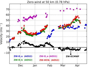
Fig. 5.Zero-wind for bias correction derived at 50 km from the

O3line in band-A using spectrometer 1 (magenta dots) and

spec-trometer 2 (blue dots), the O₃line in band-B and spectrometer 2 (green dots) and HCl line in band-B (red dots) along with the zero-wind computed with the paired ECMWF zero-winds. The error bar cor-responds to the retrieval errors of the averaged profiles (1-σ). The zero-wind includes the subtraction of the ECMWF zero-winds.

ECMWF winds. Figure 5 shows the zero-winds at 50 km de-rived from the three SMILES products. At this altitude, the three products are retrieved with a good sensitivity and the spectrometer frequency error is expected to be the main surement bias. For lines in band-B, which is always mea-sured with the second spectrometer unit (AOS-2), the zero-wind corrections vary between 20–50 m s−1_{and the}

day-to-day changes do not exceed 5 m s−1_{. The zero-wind}

correc-tion retrieved from the O3line in band-A shows two regimes

depending which spectrometer is used. When the first spec-trometer unit (AOS-1) is used for the measurements (config-uration for measuring band-B simultaneously), the zero-wind correction values are between 50–70 m s−1. When band-A is measured with AOS-2, the zero-wind values are similar to those obtained for band-B. After removing the atmospheric wind variability estimated using ECMWF winds (ECMWF zero-wind in Fig. 5), a linear trend of∼_{20 m s}−1_{/6-months is} seen on the 4 observational configurations (not shown). This trend is compatible with the main local-oscillator stability ex-pected to be δν

ν =6.8×10

−8_{/6-months whereν is the local}

oscillator frequency. Zero-wind corrections relevant to band B oscillate with a period of 2 months and an amplitude of 10–20 m s−1_{. Although the period is compatible with that of}

the instrument thermal variation, the origin of the oscillation on the band-B zero-wind is not yet fully understood.

Such frequency offsets (<0.1 MHz) are acceptable for trace gas retrievals which are the first objective of the mis-sion. However, it is clearly not good enough for wind re-trieval which requires the “zero-wind” correction. However, as seen by the ECMWF zero-wind, during some periods

between December and February the atmospheric contribu-tion in the zero-wind correccontribu-tion can reach∼10 m s−1_which

would introduce a bias in the wind profile if solely cor-rected with the retrieved zero-wind value. Above 0.01 hPa, ECMWF winds are not available and are linearly extrapo-lated.

3 Data quality assessment and comparison with ECMWF analysis

The data quality assessment consists, first, of checking the internal consistency of the SMILES winds derived from dif-ferent spectroscopic lines and spectrometers. For further ver-ification, retrieved winds need to be compared with inde-pendent wind information. Lacking other measurements in the middle and upper stratosphere, such information is taken from the operational ECMWF analyses. It is known that, at high altitudes, tropical ECMWF winds are poorly con-strained. Baldwin and Gray (2005) have compared ECMWF ERA-40 reanalysis zonal-winds with observations from two tropical stations. They found good agreement below 2–3 hPa but, at higher altitudes, their conclusion was that the reanal-ysis winds should be used with caution (correlation of 0.3 at 0.1 hPa with observations). Although this analysis is based on an outdated version of the ECMWF (version cy23r4), these results may still be valid and highlight the difficulties for reproducing winds in the tropics. Hence, the compari-son of SMILES with ECMWF winds is not only relevant for the SMILES wind quality assessment but it also provides in-sights on the quality of the ECMWF winds themselves. For full verification of the SMILES winds, the mesospheric mea-surements should also be validated with ground-based radar observations. However, such analysis is beyond the scope of this paper.

3.1 Internal consistency check

The upper panels of Fig. 6 show the mean meridional wind profiles in 20◦ latitude bins between 20◦S and 60◦N that have been retrieved from the O3lines in bands A and B (blue

and green lines, respectively) and from the HCl line in band B (red line). Only measurements when bands A and B were measured simultaneously are used. This corresponds to one third of the full dataset. The retrieved winds have been cor-rected with the zero-wind profile.

Between 4 and 0.1 hPa, good agreement is found for winds retrieved from the O3lines in all latitude bands. The standard

deviation of the retrieved winds (Fig. 6, lower panels) also confirms the good agreement between the O3 retrievals in

this altitude range. At lower (8–4 hPa) and upper (<0.1 hPa) altitudes, O3line derived winds exhibit differences that reach

∼_{10 m s}−1_{at higher latitudes.}

-10 0

10

Mean (ms

)

10

10

10

10

10

Pressure (hPa)

(a) 20

S

0

-10 0

10

Mean (ms

)

(b) 0

20

N

-10 0

10

Mean (ms

)

(c) 20

N

40

N

-10 0

10

Mean (ms

)

(d) 40

N

60

N

10 20 30

STD (ms

)

10

10

10

10

10

Pressure (hPa)

10 20 30

STD (ms

)

10 20 30

STD (ms

)

10 20 30

STD (ms

)

Fig. 6.Upper panels: zonally averaged near meridional wind profiles retrieved from simultaneous measurements of the spectral lines: O3

-band A (blue line), O3-band B (red line) and HCl-band B (green line). Lower panels: same as the upper panels but showing the standard

deviation of the retrieved profiles. The results for the paired ECMWF winds component along the line-of-sights are also shown (black line). Data with a line-of-sight orientation between±10◦from the meridional direction are used.

preferred. Between 1 and 0.1 hPa, the mean and the standard deviation of the profiles retrieved from the HCl line (dashed-red line) match those from the O3retrievals. At higher

alti-tudes, the mean and standard deviation of the HCl wind pro-files smoothly expands up to 0.005 hPa. In the lower part of the retrieval range (>1 hPa), large differences with O3

re-trievals can be seen as expected from the degradation of the accuracy and the precision of the HCl line retrieval.

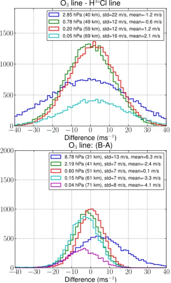
The upper panel of Fig. 7 shows the differences between profiles retrieved from the O3and the HCl lines in band-B

be-tween 40 and 70 km. At 50 and 60 km, the standard deviation and the mean of the differences are 12 m s−1and<1.2 m s−1, respectively. Since both profiles are derived from simultane-ous measurements with the same spectrometer, the standard deviation is representative of the errors due to the measure-ment thermal noise. The value is consistent with the theo-retical estimate: 5–8 m s−1_{and 10 m s}−1_{for O}

3and HCl

re-trievals, respectively. At 70 km, the standard deviation in-creases to 16 m s−1 _{which is also consistent with the loss}

of precision for both O3 and HCl retrievals (20 m s−1 and

13 m s−1, respectively). The value of 16 m s−1is smaller than

the standard-deviation expected from the theoretical errors (root-sum-square of the errors is 24 m s−1) indicating a pes-simistic estimate of the theoretical error from the O3 line.

The actual mean precision of the winds derived from O3is

likely between 12–15 m s−1_{. Above 70 km (0.05 hPa), ozone}

has strong diurnal and latitudinal variations (Kasai et al., 2013) which induce large variations of the O3line intensity

of more than an order of magnitude, and therefore, of the wind retrieval precision.

The comparison of the winds derived from the ozone line simultaneously measured in bands A and B (different spec-trometers) and corrected with the zero-wind technique is shown in Fig. 7 (lower panel). The mean difference at alti-tudes between 40–60 km is less than 3 m s−1and the standard deviation of the differences is 7 m s−1. At 30 km, the mean difference and the standard deviation increase to 6 m s−1and 13 m s−1_{, respectively. Since the profiles are retrieved from}

−40 −30 −20 −10 0 10 20 30 40

Difference (ms−1₎

0 500 1000 1500

O3line - H 35

Cl line

2.85 hPa (40 km), std=22 m/s, mean=-1.2 m/s 0.78 hPa (49 km), std=12 m/s, mean=-0.6 m/s 0.20 hPa (59 km), std=12 m/s, mean=1.2 m/s 0.05 hPa (69 km), std=16 m/s, mean=2.1 m/s

−40 −30 −20 −10 0 10 20 30 40

Difference (ms−1)

0 500 1000 1500

2000 O3line: (B-A)

8.78 hPa (31 km), std=13 m/s, mean=6.3 m/s 2.19 hPa (41 km), std=7 m/s, mean=-2.4 m/s 0.60 hPa (51 km), std=7 m/s, mean=0.1 m/s 0.15 hPa (61 km), std=7 m/s, mean=-3.3 m/s 0.04 hPa (71 km), std=8 m/s, mean=-4.1 m/s

Fig. 7.Upper panel: histogram of differences of the velocity re-trieved from the O3and the HCl lines in band B. Lower panel: same

as for the left panel but for line-of-sight winds retrieved from the O3

lines in bands A and B measured simultaneously. Data for latitudes between 20◦N and 60◦N have been used.

retrieval to another. Hence, the residual errors from the spec-trometer channels frequency after the zero wind correction can be assumed as a random retrieval error of∼_{5–7 m s}−1_.

In conclusion, the different SMILES products agree with each other in the mid- and upper stratosphere where the re-trieval performances are similar for each product. Our results also confirm that winds retrieved from the O3line should be

used between 8–0.1 hPa while those obtained from the HCl line retrievals should be used between 0.1–0.01 hPa. The ac-tual precision is significantly worse than the theoretical com-putation because of a residual error after the zero-wind cor-rection. An additional noise of 5 m s−1likely arises from the fluctuation in the spectrometer frequency errors. Taking into account this additional noise, the total precision of the wind

retrieval becomes 7–9 m s−1_{in the middle and upper}

strato-sphere.

3.2 Comparison with the ECMWF meridional component

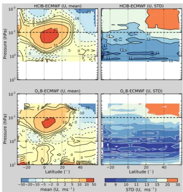
The internal checks presented in the previous section do not allow us to estimate the errors due to the platform veloc-ity, and to the local-oscillator frequency, which affect the three wind products in the same way. However, in the trop-ics and extra-tropical stratosphere where meridional veloc-ities are weak (Fig. 6), the differences between ECMWF and SMILES single profiles are caused by the retrieval er-rors, and, to a lesser extent, by coincident and non-simultaneous profile pairing and by uncertainties of ECMWF analysis. Hence the analysis of the differences between SMILES and ECMWF meridional winds in the stratosphere allows us to verify the wind retrieval error estimations. Note that large oscillations are seen on the SMILES wind profiles at low and mid-latitudes of the Northern Hemisphere which are likely due to atmospheric tides. In the mesosphere, the oscillations are significantly smaller in the ECMWF wind profiles and, consequently, the ECMWF standard deviations underestimate the actual winds variability in the mesosphere. The mean and the standard deviation of the differences (SMILES-ECMWF) have been calculated in latitude bins of 5◦ for data between November 2009 and April 2010, and with a line-of-sight within±₁₀◦_{around the meridional} di-rection. We rejected the days when fewer than 10 profiles were used to construct the zero-wind profile. Figure 8 (lower panels) shows the results for the data retrieved from the O3

line in band B. Over most of the region between 5–0.5 hPa, the bias between the model and the measurement (left panel) is less than 2 m s−1and the standard deviation (right panel) is less than 10 m s−1. However, the bias in the tropics should be taken with caution since the mean ECMWF tropical merid-ional wind is included in the zero-wind. According to these results, the precision (standard deviation) and the accuracy (bias) for a single retrieved profile cannot exceed 10 m s−1 and 2 m s−1, respectively, which is consistent with the error estimation.

At high latitudes (40–60◦N), a mean difference of 2– 5 m s−1 is found at 4–3 hPa which may arise from the in-crease of the measurement bias and also from the larger vari-ability of the meridional winds (Fig. 6). At lower altitudes (>8 hPa) and outside the tropics, the large mean differences are due to measurement calibration errors. The calibration errors are found to be larger for the O3 line band-A

re-trieval (not shown). In the mesosphere, above 0.3 hPa, results from the O3and the HCl lines (lower and upper panels,

10-2

10-1

100

101

Pressure (hPa) -5

-5 -5 -5 -2 -2 -2 -2 -2

0 ₀

0 0

2 2

2 2 2

5 5

5 5 10

HClB-ECMWF (V, mean)

10

10 _{10 10} 10

11 11 11 11 11 13 13 13 15 20 20 20 20 20 20

HClB-ECMWF (V, STD)

20 0 20 40

Latitude (◦)

10-2 10-1 100 101 Pressure (hPa) -20 -10-5 -5 -2 _-2 -2 0 0 0 0 0 0

2 2

2 2

2 2

2 ₂

2

5 5

5

10 10

20 20

50 ₅₀

O3B-ECMWF (V, mean)

20 0 20 40

Latitude (◦)

8 8 8 9 9 ₉ 9

9

9

10

10 10 10

10 10 11 11 13 13 ₁₃ 15 15 15 ₁₅ 20 20 30

O3B-ECMWF (V, STD)

50 20 10 5 2 0 2 5 10 20 50

mean (V, ms−1) 8 9 10 11 13 15 20 30STD (V, ms−1)

Fig. 8. Comparison of the near meridional winds retrieved from

band-B with the operational ECMWF analysis. Data with a line-of-sight orientation between±10◦from the meridional direction are used and ECMWF winds are projected along the line-of-sight direction. Upper panels: mean (left panel) and standard deviation (right panel) of the differences for profiles retrieved from the HCl lines. Lower panels: same as for the upper panels but for profiles retrieved from the O₃line. Data between November 2009 to April 2010 have been selected.

For instance Morton et al. (1993) has reported migrating-tides induced meridional wind oscillations above 60 km dur-ing the winter solstice and predominantly near 20◦_{N. Below} 80 km, the tides amplitude and the vertical wavelength was about 40 m s−1_{and 20 km, respectively.}

3.3 Comparison with the ECMWF zonal component

In Fig. 9, the same methodology as in the previous section is applied for deriving the mean and standard deviation of differences between SMILES (band-B) and ECMWF zonal (±₁₀◦_{) winds. Zonal winds are in general significantly larger} than the meridional ones, and thus, the results are more sen-sitive to mismatches due to profile pairing and ECMWF un-certainties.

As for the meridional component, large mean differences, likely due to intensity calibration errors, are found at lower altitudes (>8 hPa) in the extra-tropical regions (lower right panel) and at latitudes<30◦S because of the fast rotation of the line-of-sight from the zonal to meridional direction. However, in most of the stratosphere (4–1 hPa), a low bias between±_{2 m s}−1_{is found except over the Equator where} the mean difference is between 5–10 m s−1. In the

meso-10-2 10-1 100 101 Pressure (hPa) -20 -10 -10 -5 -5 -5 -2 -2 -2

0 0 0

0 0 0 0 2 2 2 5 5

5 ₅

10 10

20

HClB-ECMWF (U, mean)

10

11 11 11

11

13 13

13 13 13

15 15

20 20 20HClB-ECMWF (U, STD)20 20

20 0 20 40

Latitude (◦)

10-2 10-1 100 101 Pressure (hPa) -20 -20 -10 -10 -5 -5 -5 -2 -2 -2 -2 0

0 0

0 0

0 0

2 2

2 2 2

2

5 5

5 10 10 10 20 20 20 50 50

O3B-ECMWF (U, mean)

20 0 20 40

Latitude (◦)

8 ₉

9

9 9 9

9 9 10 10 10 10 10₁₀ 11 11 11 13 13 13 15 15 1515 15 20 20 30

O3B-ECMWF (U, STD)

50 20 10 5 2 0 2 5 10 20 50

mean (U, ms−1) 8 9 10 11 13 15 20 30STD (U, ms−1)

Fig. 9.Same as for Fig. 8 but for the near zonal component. Data with a line-of-sight orientation between±10◦from the zonal direc-tion are used.

sphere (1–0.01 hPa, upper right panel), a large positive dif-ference (20–30 m s−1) is found in the tropics and a nega-tive difference at higher northern latitudes (between−20 and −10 m s−1_).

The standard deviations from the middle-stratosphere to lower mesosphere (lower right panel) are slightly higher than the values found for the meridional components. Such an increase of the standard deviation is consistent with the in-crease of uncertainties in profile-pairing and in ECMWF winds. However, values below 10 m s−1 are still found over wide regions and more particularly in the extra-tropics indi-cating that SMILES captured the large variations of the zonal winds (−_{70 to +70 m s}−1_{) with a precision which is} consis-tent with the estimation of 7–9 m s−1. In the tropical meso-sphere (0.1–0.01 hPa, upper panels), the standard deviation is between 15 and 20 m s−1which also corresponds to the re-trieval precision. At northern mid-latitudes, the mesospheric standard deviation significantly increases to 20–30 m s−1_,

likely due to the increase of errors in profile-pairing and of the ECMWF analysis itself.

Although, the current SMILES observations cover a short pe-riod, some persistent biases in the analysis during the whole winter are clearly seen and SMILES could help to understand their origin. In particular, the observations can provide new constraints on the parameterisation of unresolved waves for the analysed winter which might be applied to other years. However, such investigations are out of the scope of this anal-ysis.

4 Examples of the observed wind fields

4.1 Monthly variation of zonal-winds

Figure 10 shows the zonally and monthly averaged zonal-winds obtained from band-B between 30◦_S–55◦_{N and from} mid-October to mid-April. Information at lower altitudes

>0.1 hPa (<65 km) is retrieved from the O3 line and that

for the upper altitudes is from the HCl triplet. Until the first week of November, ECMWF were not available to us and the zero-wind correction has been calculated with winds from the version 5.2 of the analysis of the Goddard Earth Ob-serving System Data Assimilation System model (GEOS-5.2) (Reinecker, 2008). In November and February, the ob-served latitude range is displaced to about 60◦S–30◦N be-cause of the 180◦–maneuver of the ISS when hosting the space shuttle. The space shuttle also docked in April, but the viewing geometry did not allow the construction of “zero-wind” profiles. Since the Southern Hemisphere observations corresponded only to a few days, it has been decided to only focus on the region observed in the normal operation mode (30◦_S–55◦_N).

The monthly climatology exhibits the main and well known characteristics of the seasonal variations of the zonal-winds. Near the equinoxes (October, March and April), in the stratosphere and the lower mesosphere, zonal-winds are primarily eastward. In December and January, they become stronger with a large inter-hemispheric contrast: eastward in the winter-time Northern Hemisphere and westward in the summer-time Southern Hemisphere.

In the tropical upper-stratosphere and mesosphere (<3 hPa), the main characteristics of the Semi-Annual-Oscillation (SAO) in the zonal-winds are seen with, in partic-ular, the opposite phase between the stratosphere (westward in December) and the mesosphere (eastward in December). At lower altitudes (>4 hPa), the SAO signal vanishes and is dominated by the Quasi-Biennal Oscillation (QBO) which is in an easterly phase (westward winds) during that period. The observed tropical SAO is discussed in more details in Sect. 4.3.

Though the Arctic region is not observed by SMILES, the zonal winds in the northernmost mid-latitudes (45–55◦N) are high westerlies during winter (e.g. in December and Jan-uary) revealing the edge of the Arctic polar Vortex. The dy-namics of the Arctic winter 2009/2010 have been described

10-2 10-1 100 -40 -30 -30 -30 -20 -20 -10 -10 0 0

10 10 10

10 10 20 20 20 20 30 30 30 40 40 40 40 6090 October 2009 -30 -30 -20 -20 -10 -10 0 0 10 10 20 20 20 30 30 30 30 40 40 40 40

60 ₆₀₉₀

November 2009 -60 -40 -30 -20 -20 -10 -10 0 0 10 10 20 30 30 40 40 40 60 60 60 90 December 2009 10-2 10-1 100

Pressure (hPa) -60 -40

-30 -30

-20 -20 -10 0 -10 0 10 10 10 20 20 20 30 30 30 30 40 40 40 60 60 90 January 2010

20 0 20 40

Latitude (◦)

-40-30 -20 -20 -20 -10 -10 0 0 10 10 20 20 30 30 40 40 60 60 90 February 2010

20 0 20 40

Latitude (-40-30 ◦)

-30 -20 -20 -10 -10 -10 0 0 0 10 10 10 20 20 20 30 30 30 30 40 40 40 40 60 90 March 2010

20 0 20 40

Latitude (◦)

10-2 10-1 100 -40-30 -20 -20 -10 -10 0 0 0

10 10 10

10 20 20 20 30 30 40 40 60 90 April 2010

90 60 40 30 20 10 0 10 20 30 40 60 90

U (ms−1)

Fig. 10. Monthly and zonally averaged near zonal-wind derived

from SMILES measurements in band B between October 2009 to April 2010. Wind information is taken from the O₃line retrieval for altitudes below 0.1 hPa (65 km) and from the HCl line retrieval above. Data with a line-of-sight orientation between±10◦from the zonal direction are used.

in several studies (Wang and Chen, 2010; D¨ornbrack et al., 2012; Kuttippurath and Nikulin, 2012). In early winter, plan-etary wave activity prevented the formation of a strong vortex in the lower stratosphere and the vortex eventually split at the beginning of December (minor stratospheric warming). From December onward, the vortex became strong through-out the stratosphere until a major sudden stratospheric warm-ing (SSW) occurred on 24–26 January 2010. After this event, a weak vortex reformed and disappeared in April. It is shown in Sect. 4.2 that the effects of the two SSW are observed at 2 hPa in the daily variation of the mean zonal-wind between 50◦N and 55◦N. Hence, SMILES offers direct wind mea-surements for studying the SSW development from the mid-stratosphere (8 hPa) to the mesosphere as well as the interac-tions with the mid-latitudes.

4.2 The sudden stratospheric warming events

The effects of the major SSW at ∼_{5 hPa (}∼_{36 km) are} clearly seen in Fig. 3. The coloured background indicates the abundance of N2O from a dynamical model driven by

ECMWF winds on the 850 K surface and constrained by Odin/SMR observations (R¨osevall et al., 2007). The polar vortex is characterised by low values of N2O (blueish colour)

2 January 2010, the vortex is well centred above the polar region and strong eastward winds are measured on its periph-ery. The meridional component is alternatively southward or northward following the vortex meanders. On 26 January, the vortex is displaced over the north of Europe and it is confined between 60◦W and 120◦E. Inside the vortex, SMILES ob-served the change of the direction of the meridional winds due to the counterclockwise rotation of the flow. Outside the vortex a westward flow is measured due to an anti-cyclonic system located above the pacific.

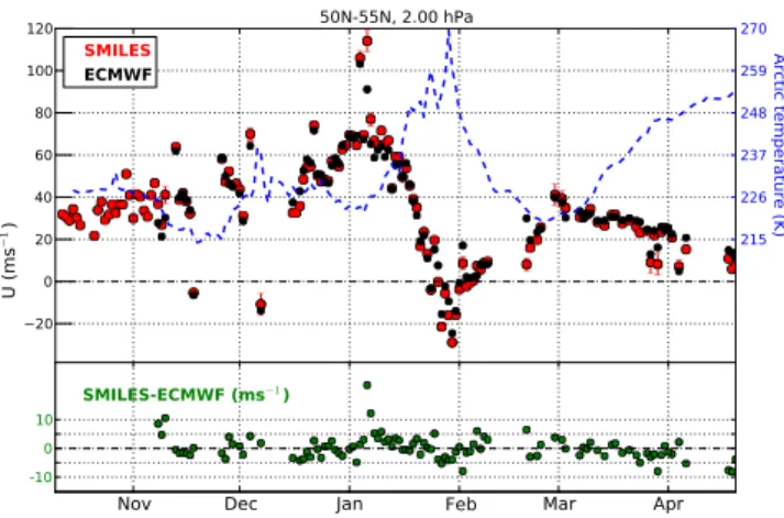
Figure 11 (red dots) shows the daily variation at∼_{2 hPa of} zonally averaged zonal-winds measured between 50–55◦N. The time series is made from the O3 line retrievals. When

both bands A and B are measured simultaneously, only band-B is used. The error bars correspond to the daily-mean preci-sione¯(1-σ):

¯

e=

s

e2

nzero

+e

2_+e2

s

nwind

, (1)

wheree=_{5 m s}−1_{is the single profile retrieval precision at} 2 hPa (Sect. 2.2),es =5 m s−1is the additional noise arising

from the zero-wind correction (Sect. 3.1) and,nzeroandnwind

are the number of profiles to construct the daily zero-wind and the mean zonal-wind, respectively. The first term below the root-square operator is added to account for the retrieval errors on the zero-wind profiles.

A minor and a major SSW occurred in the beginning of December and at the end of January, respectively. In both cases, a reversal of the mean zonal flow direction is mea-sured between 50–55◦N, accompanied by a steep increase of the temperature in the Arctic (blue dashed line). The temper-ature data are daily and zonally averaged AURA/MLS ob-servations (Schwartz et al., 2008; Limpasuvan et al., 2005) between 60–80◦N. The wind and temperature observations are consistent with the analysis of meteorological data in the Arctic of various winters (Labitzke and Kunze, 2009; Manney et al., 2009; D¨ornbrack et al., 2012). In the begin-ning of January, when the vortex had the strongest intensity, the mean eastward zonal-winds strongly increased to 60– 80 m s−1. Then, the flow direction gradually changed until the end of January (−_{20 m s}−1_{). The flow returned to a} nor-mal eastward direction in few days and reached a maximum velocity of 40 m s−1in the beginning of March and decreased again when the vortex disappeared in the springtime.

The ECMWF zonal-winds (Fig. 11, black dots) are consis-tent with the measurements. A good agreement (difference

<5 m s−1) is found on average. The largest differences (10– 15 m s−1) are found in beginning of November and January when the vortex was strongest.

4.3 Zonal wind development in the tropics

Figure 12 shows the daily-averaged zonal-wind over the Equator (±₅◦_{) using the same averaging method as in}

Nov Dec Jan Feb Mar Apr

20 0 20 40 60 80 100 120

U (

ms

−

1)

50N-55N, 2.00 hPa

SMILES

ECMWF

215 226 237 248 259 270

Arctic temperature (K)

-100

10 SMILES-ECMWF (ms

−1)

Fig. 11.Upper panel: daily-averaged SMILES zonal-wind in the

northern high-latitudes at 2 hPa (∼41 km) (red dots) and ECMWF analyses (black dots) between 50–55◦N. SMILES winds are re-trieved from the O3line measured in band-B or in band-A if B is

not measured. Data with a line-of-sight orientation between±10◦ from the zonal direction are used. ECMWF winds are projected on the line-of-sight. Temperature information (blue dashed line) is based on daily and zonally averaged MLS measurements between 60–80◦N. Lower panels: difference SMILES-ECMWF.

Sect. 4.2. When band-B is measured, data above 0.1 hPa are replaced by the HCl line retrievals. The downward progres-sion from the lower mesosphere to the middle stratosphere of the eastward phase (reddish colour) is typical of the winter SAO signal (Hirota, 1980; Garcia et al., 1997). A large vari-ation in amplitude is measured at the stratopause (∼1 hPa) where a complete reversal of the wind direction occurred: +20 m s−1 _{(eastward) in November, −60 m s}−1 _{in January}

and +20 m s−1_{in April. In the mesosphere (0.1–0.007 hPa),}

the dataset, based on the HCl line measured in band-B, is quite sparse. It shows that the wind flow also varies over a large velocity range (between−_{60 and +60 m s}−1_{) but, as} expected, the wind direction changes in anti-phase with the stratosphere (Hitchman et al., 1997; Lossow et al., 2008).

At lower altitudes (below 5 hPa), the SAO amplitude de-creases and is mixed with the QBO (Hirota, 1980; Baldwin and Gray, 2005). The westward flow measured over most of the period below 5 hPa is consistent with the easterly (west-ward) phase of the QBO during the SMILES period. Unfor-tunately the time period observed is too short to see a full cycle of the QBO.

Figure 13 shows the comparison with ECMWF analysis of daily-averaged zonal-winds at 4, 2 and 0.2 hPa (35, 40, and 60 km) between 15◦_S–15◦_{N. The error bars correspond to} the precision of the daily-averaged profiles (see Sect. 4.2) as-suminge=_{7, 5 and 7 m s}−1_andes=7, 5 and 5 m s−1 for

Nov Dec

Jan

Feb Mar Apr

10-2

10-1

100

Pressure (hPa)

Equatorial zonal wind (ms

)

60 50 40 30 20 10 0 10 20 30 40 50 60

Fig. 12. The Semi-annual oscillation of the zonal winds over

the equator (±5◦). Red regions correspond to eastward (westerly) winds. The winds from both the ozone and HCl lines are combined in the plot when band-B is measured: information is for O3line

be-low 0.1 hPa (65 km) and from HCl above. Information is from O₃ when only band-A is measured. Data with a line-of-sight orientation between±10◦from the zonal direction are used.

the Northern Hemisphere. For instance at 2 hPa, winds vary between−_{60 and 30 m s}−1_{on the southern side of the} equa-tor and between−_{30 and 40 m s}−1_{on the northern side.} Un-like the QBO signal in the zonal wind which is nearly sym-metric about the equator (Hamilton et al., 2004), rockets and HRDI observations have reported an asymmetry in the upper-stratospheric SAO with a stronger amplitude in the southern tropics (Hirota, 1980). This is consistent with the SMILES observations. Because of the increase of the SAO with al-titude, the wind variation is larger in the upper-stratosphere (2 hPa) than in the mid-stratosphere (4 hPa).

In the stratosphere (4 and 2 hPa), the ECMWF analyses reproduce the measurements fairly well. However, at 2 hPa, the variation range within time intervals as short as about 1 week is larger in the measurements by 20–30 m s−1_{. In}

par-ticular, the strong increase of the westward zonal-winds mea-sured during the two first weeks of February in both hemi-spheres is not seen in the ECMWF analyses. On the con-trary, at this time, the ECMWF winds start the westward-to-eastward flow transition. Daily and zonally averaged MLS temperatures for the same latitude range are shown along with the winds. The signature of the SAO in the tempera-ture is in phase with the winds SAO: warmer temperatempera-ture during the eastward flow and cooler temperature during the westward flow. Note that the transition from the cooler to warmer temperature starts ahead (end of January) compared to the measured westward-to-eastward transition of the zonal winds (beginning of February). It is during this period that the large mismatch between SMILES and ECMWF winds occurs.

40 20 0 20 40 60 80

U (

ms

−

1)

15S-Eq, 0.20 hPa

SMILES

ECMWF

Eq-15N, 0.20 hPa

60 40 20 0 20 40 60

U (

ms

−

1)

15S-Eq, 2.00 hPa Eq-15N, 2.00 hPa

Nov Dec Jan Feb Mar Apr 60

40 20 0 20 40 60

U (

ms

−

1)

15S-Eq, 4.00 hPa

Nov Dec Jan Feb Mar Apr

Eq-15N, 4.00 hPa

234 236 238 240 243 245 247

Temperature (K)

247 250 253 256 258 261 264

Temperature (K)

235 237 239 242 244 246 248

Temperature (K)

Fig. 13. Left panels: daily-averaged zonal-wind in the southern

tropics (15◦S–Eq) at 4, 2 and 0.2 hPa (∼35, 41 and 60 km) de-rived from SMILES measurements (red dots) and ECMWF analy-ses (black dots). Data are retrieved from the O3line in band-B or in

band-A if B is not measured. Data with a line-of-sight orientation between±10◦from the zonal direction are used. ECMWF winds are projected on the line-of-sight. The temperature profiles (blue dashed line) is a daily and zonal average of MLS measurements in the same latitudes range. Right panels: same as left panels but for the northern tropics.

In the lower mesosphere (0.2 hPa), the measured wind SAO is in phase with the stratospheric oscillation and the amplitudes in both hemispheres are similar (∼_{20 m s}−1_). It is also in phase with the temperature oscillation, which has the opposite phase to that of the stratospheric tempera-ture. The ECMWF winds depart significantly from SMILES winds by a constant offset of about 20 m s−1(consistent with Fig. 9). However, the amplitude of the oscillation is consis-tent with the observed one. Day-to-day variations are more pronounced in the measurements than in ECMWF winds. In particular, in the Northern Hemisphere, between November and January, the measurements exhibit an oscillation with a period of 10–20 days and an amplitude of∼20 m s−1_which

5 Conclusions

We have reported measurements of winds between 8– 0.01 hPa and 30◦S–55◦N during the northern winter 2009– 2010. Three winds products were derived from spectro-scopic measurements by the sub-mm wave limb sounder JEM/SMILES. The zonal and meridional components were retrieved from different parts of the orbit. The precision and the accuracy are 7–9 m s−1 and 2 m s−1 between 8–0.5 hPa and<20 m s−1 and<5 m s−1 in the mesosphere. The ver-tical resolution is 5–7 km from the mid-stratosphere to the lower mesosphere and <20 km elsewhere. To our knowl-edge, this is the first time that winds have been observed between 35–60 km from space. Internal comparisons show a good quantitative agreement between the different SMILES products. Good agreement is also found with the ECMWF analyses in most of the stratosphere except for the zonal-winds over the equator (mean difference of 5–10 m s−1_{). In}

the mesosphere SMILES and ECMWF zonal-winds exhibit large differences>20 m s−1, especially in the tropics. These results demonstrate that SMILES measurements have the po-tential to significantly improve the capability of atmospheric models to predict winds in the tropical mid- and upper strato-sphere, and in the mesosphere in general.

In coming work, SMILES mesospheric winds will be vali-dated using ground-based radar observations. We also expect better retrievals thanks to improvements of the calibrated ra-diances and spectrometer frequencies spectra (Ochiai et al., 2012c; Mizobuchi et al., 2012a), and of the inversion methodology (e.g. joint inversion of different lines and bands). The aim is to reliably retrieve winds down to 20– 25 km which is the theoretical limit for the SMILES mea-surements. In the mesosphere, the number of retrieved pro-files can be increased by the use of the H37Cl lines measured in band-A (though weaker than the band-B H35Cl line) and by using the nighttime O3line signal enhancement due to the

large chemical diurnal variation of O3at altitudes between

0.01–0.005 hPa.

Although the SMILES instrument was not designed for wind measurement, the retrieval performances are close to those used in Lahoz et al. (2005) for stressing the impor-tance of stratospheric wind measurements (error <5 m s−1 between 25–40 km). This indicates that a carefully designed sub-mm wave radiometer, which is mature technology, has the potential to significantly improve the prediction of wind in atmospheric models and to fill the altitude gap in the stratospheric wind measurements. The optimal specifications and the performances for such instrument are under study.

Appendix A

Retrieval procedure

The wind retrieval uses the algorithms version 2.1.5 de-veloped for retrieving temperature and gas profiles in the

SMILES level-2 research chain developed in NICT (http: //smiles.nict.go.jp/pub/data/products.html). They are based on the standard least-squares method constrained by an a pri-ori knowledge of the retrieved parameters. A zero profile is used for the wind a priori. The line-of-sight wind information is derived in a two step process using the ozone and HCl lines available in the spectra. Firstly the profiles of atmospheric constituent relevant for the spectral region, temperature and spectrum tangent-height are retrieved disregarding any spec-tral shifts due to the wind which has no significant impact on the results. Then the wind is retrieved on a 5 km vertical grid by initialising the inversion using the parameters retrieved in the first step. The vertical sampling of the retrieval grid is consistent with the information content of the spectra. Note that at the initialisation step, baseline parameters, i.e. addi-tional radiance offset and slope used to improve the mea-surement fit, are set to 0. Since, a small baseline is usually retrieved for good SMILES scans, the initialχ2(Baron et al. (2011), Eq. 2) has a relatively small value between 20–40.

The two inversion processes use a spectral window of 500 MHz around the chosen molecular lines. The forward model has been modified to include the Doppler frequency shift induced by the air parcels velocity and to compute the wind weighting functions. The frequency shift induced by the wind is included as a change of the spectroscopic lines frequency. The wind weighting functions are computed with a perturbation method for the derivation of the absorption co-efficient and with an analytic derivation of a discrete form of the radiative transfer equation (Urban et al., 2004). The fre-quency dependence of the source function (the Planck func-tion) is neglected and we assume horizontal winds along the full line-of-sight which is only true at the tangent point. Both approximations have a negligible impact on the retrieved ve-locities in the altitude range considered in the analysis.

Acknowledgements. The SMILES project is jointly led by the Japan Aerospace Exploration Agency (JAXA) and the National Institute of Information and Communications Technology (NICT, Japan). SMILES Data processing was performed with the NICT Science Cloud as a collaborative research project. We acknowledge the European Centre for Medium Range Weather Forecasts (ECMWF) and the Global Modelling and Assimilation Office (GMAO) at NASA Goddard Space Flight Center for access to model results. D. P. Murtagh and J. Urban would like to thank the Swedish National Space Board for support. P. Baron would like to thank K. Muranaga, T. Haru and S. Usui from Systems Engineering Consultants Co. (SEC) for their important contributions to the SMILES project. P. Baron would like to thank Yvan Orsolini for fruitful discussions as well as the two unknown referees and the editor for their comments and suggestions for improving the manuscript.

References

Alcayd´e, D. and Fontanari, J.: Neutral temperature and winds from EISCAT CP-3 observations, J. Atmos. Terr. Phys., 48, 931–947, 1986.

Alexander, M. J., Geller, M., McLandress, C., Polavarapu, S., Preusse, P., Sassi, F., Sato, K., Eckermann, S., Ern, M., Hert-zog, A., Kawatani, Y., Pulido, M., Shaw, T. A., Sigmond, M., Vincent, R., and Watanabe, S.: Recent developments in gravity-wave effects in climate models and the global distribution of gravity-wave momentum flux from observations and models, Q. J. Roy. Meteor. Soc., 136, 1103–1124, doi:10.1002/qj.637, 2010. Baldwin, M. P. and Dunkerton, T. J.: Propagation of the Arctic os-cillation from the stratosphere to the troposphere, J. Geophys. Res., 104, 30937–30946, doi:10.1029/1999JD900445, 1999. Baldwin, M. P. and Gray, L. J.: Tropical stratospheric zonal

winds in ECMWF ERA-40 reanalysis, rocketsonde data, and rawinsonde data, Geophys. Res. Lett., 32, L09806, doi:10.1029/2004GL022328, 2005.

Baldwin, M., Thompson, D., Shuckburgh, E., Norton, W., and Gillett, N.: Weather from the stratosphere?, Science, 301, 317– 318, 2003.

Baron, P., Urban, J., Sagawa, H., M¨oller, J., Murtagh, D. P., Men-drok, J., Dupuy, E., Sato, T. O., Ochiai, S., Suzuki, K., Man-abe, T., Nishibori, T., Kikuchi, K., Sato, R., Takayanagi, M., Murayama, Y., Shiotani, M., and Kasai, Y.: The Level 2 research product algorithms for the Superconducting Submillimeter-Wave Limb-Emission Sounder (SMILES), Atmos. Meas. Tech., 4, 2105–2124, doi:10.5194/amt-4-2105-2011, 2011.

Derber, J. and Bouttier, F.: A reformulation of the background error covariance in the ECMWF global data assimilation sys-tem, Tellus A, 51, 195–221, doi:10.1034/j.1600-0870.1999.t01-2-00003.x, 1999.

D¨ornbrack, A., Pitts, M. C., Poole, L. R., Orsolini, Y. J., Nishii, K., and Nakamura, H.: The 2009–2010 Arctic stratospheric winter – general evolution, mountain waves and predictability of an oper-ational weather forecast model, Atmos. Chem. Phys., 12, 3659– 3675, doi:10.5194/acp-12-3659-2012, 2012.

Fleming, E. L., Chandra, S., Barnett, J., and Corney, M.: Zonal mean temperature, pressure, zonal wind and geopotential height as functions of latitude, Adv. Space Res., 10, 11–59, 1990. Garcia, R. R., Dunkerton, T. J., Lieberman, R. S., and

Vin-cent, R. A.: Climatology of the semiannual oscillation of the trop-ical middle atmosphere, J. Geophys. Res., 102, 26019–26032, 1997.

Hamilton, K.: Dynamics of the tropical middle atmosphere: a tuto-rial review, Atmos. Ocean, 36, 319–354, 1998.

Hamilton, K., Hertzog, A., Vial, F., and Stenchikov, G.: Longitudi-nal Variation of the Stratospheric Quasi-Biennial Oscillation, J. Atmos. Sci., 61, 383–402, 2004.

Hays, P. B., Abreu, V. J., Dobbs, M. E., Gell, D. A., Grassl, H. J., and Skinner, W. R.: The High-Resolution Doppler Imager on the upper-atmosphere research satellite, J. Geophys. Res., 98, 10713–10723, 1993.

Hildebrand, J., Baumgarten, G., Fiedler, J., Hoppe, U.-P., Kai-fler, B., L¨ubken, F.-J., and Williams, B. P.: Combined wind measurements by two different lidar instruments in the Arc-tic middle atmosphere, Atmos. Meas. Tech., 5, 2433–2445, doi:10.5194/amt-5-2433-2012, 2012.

Hirota, I.: Observational evidence of the semiannual oscillation in the tropical middle atmosphere: a review, Pure Appl. Geophys., 118, 217–238, 1980.

Hitchman, M. H., Kudeki, E., Fritts, D. C., Kugi, J. M., Fawcett, C., Postel, G. A., Yao, C. Y., Ortland, D., Riggin, D., and Har-vey, V. L.: Mean winds in the tropical stratosphere and meso-sphere during January 1993, March 1994, and August 1994, J. Geophys. Res., 102, 26033–26052, 1997.

Holton, J. R. and Alexander, M. J.: The role of waves in the transport circulation of the middle atmosphere, in: Geophys. Monogr. Ser., vol. 123, AGU, Washington DC, 21–35, 2000.

Isaksen, L., Bonavita, M., Buizza, R., Fisher, M., Haseler, J., Leutbecher, M. and Raynaud, L.: Ensemble of data as-similations at ECMWF, ECMWF Technical Memorandum 636, available at: http://www.ecmwf.int/publications/library/do/ references/show?id=90034, 2010.

Jacobi, C., Arras, C., K¨urschner, D., Singer, W., Hoffmann, P., and Keuer, D.: Comparison of mesopause region meteor radar winds, medium frequency radar winds and low frequency drifts over Germany, Adv. Space Res., 43, 247–252, 2009.

Kasai, Y. J., Urban, J., Takahashi, C., Hoshino, S., Takahashi, K., Inatani, J., Shiotani, M., and Masuko, H.: Stratospheric ozone isotope enrichment studied by submillimeter wave hetero-dyne radiometry: observation capabilities of SMILES, IEEE T. Geosci. Remote, 44, 676–693, 2006.

Kasai, Y., Sagawa, H., Kreyling, D., Suzuki, K., Dupuy, E., Sato, T. O., Mendrok, J., Baron, P., Nishibori, T., Mizobuchi, S., Kikuchi, K., Manabe, T., Ozeki, H., Sugita, T., Fujiwara, M., Irimajiri, Y., Walker, K. A., Bernath, P. F., Boone, C., Stiller, G., von Clar-mann, T., Orphal, J., Urban, J., Murtagh, D., Llewellyn, E. J., Degenstein, D., Bourassa, A. E., Lloyd, N. D., Froidevaux, L., Birk, M., Wagner, G., Schreier, F., Xu, J., Vogt, P., Trautmann, T., and Yasui, M.: Validation of stratospheric and mesospheric ozone observed by SMILES from International Space Station, Atmos. Meas. Tech. Discuss., 6, 2643–2720, doi:10.5194/amtd-6-2643-2013, 2013.

Khosravi, M., Baron, P., Urban, J., Froidevaux, L., Jonsson, A. I., Kasai, Y., Kuribayashi, K., Mitsuda, C., Murtagh, D. P., Sagawa, H., Santee, M. L., Sato, T. O., Shiotani, M., Suzuki, M., von Clarmann, T., Walker, K. A., and Wang, S.: Diurnal variation of stratospheric HOCl, ClO and HO2at the equator:

compar-ison of 1-D model calculations with measurements of satellite instruments, Atmos. Chem. Phys. Discuss., 12, 21065–21104, doi:10.5194/acpd-12-21065-2012, 2012.

Kikuchi, K., Nishibori, T., Ochiai, S., Ozeki, H., Irimajiri, Y., Ka-sai, Y., Koike, M., Manabe, T., Mizukoshi, K., Murayama, Y., Nagahama, T., Sano, T., Sato, R., Seta, M., Takahashi, C., Takayanagi, M., Masuko, H., Inatani, J., Suzuki, M., and Sh-iotani, M.: Overview and early results of the Superconduct-ing Submillimeter-Wave Limb-Emission Sounder (SMILES), J. Geophys. Res., 115, D23306, doi:10.1029/2010JD014379, 2010. Killeen, T. L., Skinner, W. R., Johnson, R. M., Edmonson, C. J., Wu, Q., Niciejewski, R. J., Grassl, H. J., Gell, D. A., Hansen, P. E., Harvey, J. D., and Kafkalidis, J. F.: TIMED Doppler Interferometer (TIDI), optical spectroscopic techniques and instrumentation for atmospheric and space research III, Proc. SPIE, 3756, 289–301, doi:10.1117/12.366383, 1999.

2003/2004–2009/2010, Atmos. Chem. Phys., 12, 8115–8129, doi:10.5194/acp-12-8115-2012, 2012.

Labitzke, K. and Kunze, M.: On the remarkable Arctic

winter in 2008/2009, J. Geophys. Res., 114, D00I02,

doi:10.1029/2009JD012273, 2009.

Lahoz, W. A., Brugge, R., Jackson, D. R., Migliorini, S., Swin-bank, R., Lary, D., and Lee, A.: An observing system simula-tion experiment to evaluate the scientific merit of wind and ozone measurements from the future SWIFT instrument, Q. J. Roy. Me-teor. Soc., 131, 503–523, 2005.

Lastovicka, J.: Observations of tides and planetary waves in the atmosphere-ionosphere system, Adv. Space Res., 20, 1209– 1222, doi:10.1016/S0273-1177(97)00774-6, 1997.

Limpasuvan, V., Wu, D. L., Schwartz, M. J., Waters, J. W., Wu, Q., and Killeen, T. L.: The two-day wave in EOS MLS tempera-ture and wind measurements during 2004–2005 winter, Geophys. Res. Lett., 32, L17809, doi:10.1029/2005GL023396, 2005. Lossow, S., Urban, J., Gumbel, J., Eriksson, P., and Murtagh, D.:

Observations of the mesospheric semi-annual oscillation (MSAO) in water vapour by Odin/SMR, Atmos. Chem. Phys., 8, 6527–6540, doi:10.5194/acp-8-6527-2008, 2008.

Maekawa, Y., Fukao, S., Yamamoto, M., Yamanaka, M. D., Tsuda, T., Kato, S., and Woodman, R. F.: First observation of the upper stratospheric vertical wind velocities using the Ji-camarca VHF radar, Geophys. Res. Lett., 20, * 2235–2238, doi:10.1029/93GL02606,

1993.-Manney, G. L., Schwartz, M. J., Kr¨uger, K., Santee, M. L., Pawson, S., Lee, J. N., Daffer, W. H., Fuller, R. A., and Livesey, N. J.: Aura Microwave Limb Sounder observations of dynamics and transport during the record-breaking 2009 Arctic stratospheric major warming, Geophys. Res. Lett., 36, L12815, doi:10.1029/2009GL038586, 2009.

Marshall, A. G. and Scaife, A. A.: Impact of the QBO on surface winter climate, J. Geophys. Res., 114, D18110, doi:10.1029/2009JD011737, 2009.

McDade, I. C., Shepherd, G. G., Gault, W. A., Rochon, Y. J., McLandress, C., Scott, A., Rowlands, N., and Buttner, G.: The stratospheric wind interferometer for transport studies SWIFT), in: Igarss 2001: Scanning the Present and Resolving the Fu-ture, Vol. 3, Proceedings, 1344–1346, Sydney NSW, 9–13 July, doi:10.1109/IGARSS.2001.976839, 2001.

Merino, F., Murtagh, D., Ridal, M., Eriksson, P., Baron, P., Ri-caud, P., and de la Noe, J.: Studies for the Odin Sub-Millimetre Radiomoter: III. Performance simulations, Can. J. Phys., 80, 357–373, doi:10.1139/P01-154, 2002.

Mizobuchi, S., Ozeki, H., Kikuchi, K., Ochiai, S., Baron, P., and Nishibori, T.: Improvement in calibration algo-rithm of the AOS (acousto-optical spectrometer) using in-orbit measurement data, Geoscience and Remote Sens-ing Symposium (IGARSS), 2012 IEEE Internationa 4695– 4698, doi:10.1109/IGARSS.2012.6350417, available at: http:// igarss12.org/, 2012a.

Mizobuchi, S., Kikuchi, K., Ochiai, S., Nishibori, T., Sano, T., Tamaki, K., and Ozeki, H.: In-orbit measurement of the AOS (Acousto-Optical Spectrometer) response using fre-quency comb signals, IEEE J. Sel. Top. Appl., 5, 977–983, doi:10.1109/JSTARS.2012.2196413, 2012b.

Morton, Y. T., Lieberman, R. S., Hays, P. B., Ortland, D. A., Mar-shall, A. R., Wu, D., Skinner, W. R., Burrage, M. D., Gell,

D. A., and Yee, J.-H.: Global mesospheric tidal winds observed by the high resolution Doppler imager on board the Upper Atmo-sphere Research Satellite, Geophys. Res. Lett., 20, 1263–1266, doi:10.1029/93GL00826, 1993.

Nezlin, Y., Rochon, Y., and Polavarapu, S.: Impact of tropospheric and stratospheric data assimilation on mesospheric prediction, Tellus A, 61, 154–159, doi:10.1111/j.1600-0870.2008.00368.x, 2009.

Niciejewski, R., Wu, Q., Skinner, W., Gell, D., Cooper, M., Marshall, A., Killeen, T., Solomon, S., and Ortland, D.: TIMED Doppler interferometer on the Thermosphere Iono-sphere MesoIono-sphere Energetics and Dynamics satellite: data product overview, J. Geophys. Res.-Space, 111, A11S90, doi:10.1029/2005JA011513, 2006.

Ochiai, S., Kikuchi, K., Nishibori, T., and Manabe, T.: Gain nonlinearity calibration of submillimeter radiometer for JEM/SMILES, IEEE J. Sel. Top. Appl., 5, 962–969, doi:10.1109/JSTARS.2012.2193559, 2012a.

Ochiai, S., Kikuchi, K., Nishibori, T., Manabe, T., Ozeki, Hi-royuki Mizobuchi, S., and Irimajiri, Y.: Receiver performance of Superconducting Submillimeter-Wave Limb-Emission Sounder (SMILES) on the international space station, IEEE T. Geosci. Remote, 99, 1–12, doi:10.1109/TGRS.2012.2227758, 2012b. Ochiai, S., Nishibori, T., Kikuchi, K., Mizobuchi, S., Manabe, T.,

Mitsuda, C., Baron, P., and Ueno, S.: Tangent height accuracy of superconducting Submillimeter-Wave Limb-Emission Sounder (SMILES) on International Space Station (ISS), Geoscience and Remote Sensing Symposium (IGARSS), 2012 IEEE Interna-tional, 1290–1293, doi:10.1109/IGARSS.2012.6350824, avail-able at: http://igarss12.org/, 2012c.

Orr, A., Bechtold, P., Scinocca, J., Ern, M., and Janiskova, M.: Improved Middle Atmosphere Climate and Forecasts in the ECMWF Model through a Nonorographic Gravity Wave Drag Parameterization, J. Climate, 23, 5905–5926, 2010.

Ortland, D. A., Skinner, W. R., Hays, P. B., Burrage, M. D., Lieber-man, R. S., Marshall, A. R., and Gell, D. A.: Measurements of stratospheric winds by the High Resolution Doppler Imager, J. Geophys. Res., 101, 10351–10363, 1996.

Polavarapu, S., Shepherd, T. G., Rochon, Y., and Ren, S.: Some challenges of middle atmosphere data assimilation, Q. J. Roy. Meteor. Soc., 131, 3513–3527, doi:10.1256/qj.05.87, 2005. Randel, W., Udelhofen, P., Fleming, E., Geller, M., Gelman,

M., Hamilton, K., Karoly, D., Ortland, D., Pawson, S., Swinbank, R., Wu, F., Baldwin, M., Chanin, M.-L., Keck-hut, P., Labitzke, K., Remsberg, E., Simmons, A., and Wu, D.: The SPARC Intercomparison of Middle-Atmosphere Climatologies, J. Climate, 17, 986–1003, doi:10.1175/1520-0442(2004)017<0986:TSIOMC>2.0.CO;2, 2004.

Reinecker, M.: The GEOS-5 data assimilation system: A documen-tation of GEOS-5.0, Tech Report 104606 V27, NASA, 2008. R¨osevall, J. D., Murtagh, D. P., Urban, J., and Jones, A. K.: A

study of polar ozone depletion based on sequential assimilation of satellite data from the ENVISAT/MIPAS and Odin/SMR in-struments, Atmos. Chem. Phys., 7, 899–911, doi:10.5194/acp-7-899-2007, 2007.