On impatience, education, returns, and inequality

FUNDAÇAO GETULIO VARGAS

_,

-ESCOLA de POS-GRADUAÇAO em

ECONOMIA

Guido Couto Penido Guimarães

On Impatience, Education, Returns,

and Inequality

Rio de Janeiro

On Impatience, Education, Returns,

and Inequality

Dissertação para obtenção do grau de

mestre apresentada

à

Escola de

Pós-Graduação em Economia

Área de concentração: Macroecono··

1m a

Orientador: Pedro Cavalcanti

Fer-reira

Rio de Janeiro

Guimarães, Guido Couto Penido

On impatience, education, returns, and inequality f Guido Couto Penido Guimarães. - 2015.

38 f.

Dissertação (mestrado)- Fundação Getulio Vargas, Escola de Pós-Graduação em Economia.

Orientador: Pedro Cavalcanti Ferreira. Inclui bibliografia.

1. Modelos macroeconômicos. 2. Educação e nível de renda. 3. Renda-Distribuição. 4. Igualdade. S. Programas de sustentação de renda. I. Ferreira, Pedro Cavalcanti. 11. Fundação Getulio Vargas. Escola de Pós-Graduação em Economia. Ill. Título.

GUIDO COUTO PENIDO GUIMARÃES

ON IMPATIENCE, EDUCATION, RETURNS, ANO INEQUALITY.

Dissertação apresentada ao Curso de Mestrado em Economia da Escola de Pós-Graduação em Economia para obtenção do grau de Mestre em Economia,

Data da defesa: 13/04/2015

ASSINATURA DOS MEMBROS DA BANCA EXAMINADORA

Pedro Cavalcanti tfomes Ferretra Orientadér (a)

XX páginas

Dissertação (Mestrado) - Escola de Pós-Graduação em Economia.

1. DSG E lvlodel

2. Calibration

In this paper we investiga te the impact of initial wealth anel impatience heterogeneities,

as wcll as differential access to financia! markets on povcrty anel inequality, anel cvaluate

some mechanisms that could be used to alleviate situations in which these two issues are

alarming.

To address our qucstion we develop a dynamic stochastic general cquilibrium modo!

of educational anel savings choicc with heterogeneous agents, where individuais differ in their initial wealth anel in their discount factor. We find that, in the long run, more

patient households tend to be wealthier anel more educated. However, our baseline model

is not able to give as much skewness to our income distribution as it is rcquircd. We then propose a novel returns structure based on empírica! observation of heterogeneous returns

to different portfolios. This modification solves our previous problem, evidencing the im-portance of the changes made in explaining the existing levels of inequality. Finally, we

introducc two kinds of cash transfers programs- one in which receiving thc benefit is

con-ditional on educating the household's youngster (CCTS) anel one frec of concon-ditionalities

(CTS) - in order to evaluate the impact of these programs on the variables of concern1 Wc fine! that both policies have similar qualitativo rcsults. Quantitatively, howcvcr, the

CCTS outperforms its unconclitional version in all fielcls analyzecl, revealing itself to be a preferable policy.

Keywords: DSGE moclel, eclucation, inequality, misery, impatience.

1_{That is, poverty, inequality and educat.ion.}

1 Introduction

2 Basic Mo dei of Educational Choice

2.1 The Agents 2.2 The Finn

3 The Recursive Model

3.1 OLG Extension ..

3.2 Rccnrsivc Formnlation 3.3 Equiliurium . . . .

3.4 Introducing Transfers .

4 Calibration & Results 4.1 Calibration lvlcthodology 4.2 Parameters Choice

4.3 Calibration Results .. 4.3.1 Basclinc Model

4.3.2 Baseline moclel with CTS

4.3.3 Baseline moclcl with CCTS . 4.4 Heterogeneous Returns Structure

4.4.1 Modcl lvlodification . . . .

4.4.2 Calibration . . . .

4.4.3 Results Hcterogeneous Returns Model

4.4.4 Hetcrogeneous Rcturns Modcl with CTS

4.4.5 Heterogeneous Returns lvlodel with CCTS 4.5 Robustncss Check: Progressive Taxation . . . . .

5 Conc!usion

6 11 11 12 14 14 14 17 17 19 19 19 21 21 22 24 25 25 27 28 29 30 31 33

6 Appendix A 34

1

Introduction

The factors behind the existence of the huge world's inequality and poverty have been a

major concern for economists in recent years. They are vast and have been investigated by severa! authors. Some of them are the lack of good institutions (OECD (2011), Acemoglu

and H.obinson (2014)), organized interest groups associated with government corruption

(Gupta et. ai (1998), Gilens and Page(2014)), financialization (Lin and Devey(2011)) and even bequest (Kotlikoffand Summers(1981), Gale and Scholz(1994)) and entrepreneurship

(Gentry and Hnbbard(2004), Quadrini(1999 and 2009)) bchavior.

In this paper wc focns on the role edncational choices and savings behavior play on generating these undesirable outcomes. More specifically, we focns on the impact of

impa-tience and initial wealth heterogeneities, as well as differential access to financiai markets on edncational and savings choiccs of the agents, and then analyzc thc consequences of

this interaction on the income and wealth distributions, incidence of poverty and human capital. 'vVe are also interested in evaluating some mechanisms that could be nsed to

alleviate sitnations in which thesc variables are alarming. Here we evalnatc two kinds of

cash transfers programs - one in which receiving the benefit is COIH.Iitional on educating

the honsehold's youngster (CCTS) and one free of conditionalities (CTS).

To address our question we develop a dynamic stochastic general equilibrium moclel of

education anel savings choicc with heterogencous agents, whcrc individuais diffcr in their initial wealth and in their discount facto r. 2 Without claiming that the factors already

explored in the literature are not important in the choice of getting education or not, we

do not use these sources of heterogcncity because of two main rcasons: first, as wc havc already mentioned, they have been widely explored, anel second because we believe that

they are not deterrent factors: even if your parents are not educated anel you have difficulty to learn, you can succeed in trailing the educational path. Later we add differential access to financiai markets to the modcl, which helps us explain thc cxisting leveis of inequality.

Finally we introduce the cash transfers programs mentioned in order to evaluate their

impact over inequality, poverty and human capital. They are, as in Barham et. al(1995) and unlike Kong(2013), wealth proportional rich-to-poor transfcr programs.

We formulate our problem recursively anel, in order to give more variability to the income and wealth distributions, we acld an idiosyncratic zero mean shock to the worker's

productivity, which will boost the amount of precautionary savings. Taking a general cqnilibrium in thc labor markcts approach, wc include a reprcscntative compctitive firm,

which uses educated anel uneducated workers as inputs. As there is no capital in our

2_{In order to build intuition regarding the process, we proceed stcp by step when buildíng our modcl.}

\Ve first dcvclop a simple two pcriod model and cxtcnd it to an OLG structure. In these we modcl thc individual agent's problcm. Later we slightly modify thc model by aggrcgahng t.he problem into t.lw

household's problem, <tnd using the resulting dynastic strncture thereon. Our results are based on a recursivo formulation of this new problem.

country's production function we take a small open economy approach, fixing the interest ratc cqual to the "world's" onc.

The literature on the importance and the detcrminants of educational decisions is

hnge. It has explored exhaustively role of hetcrogeneous ability and parenta! educational leve! on the agcnts' cducation (Hare and Ulph(1979), Barham et al.(1995), Rcstuccia and

Urrutia(2004), del Rey and Racionero(2002), etc). The common ground between these articles is that both of the characteristics are positively correlated with the agent's

ed-ucational achievement and this is positively correlated with his future wealth. Another rcsult commonly found in thc litcrature is that rich-to-poor cash transfer schemcs tem!

to ameliorate the equilibrium inequality situation3

. In this work, however, we do not use

these heterogeneities. We focus on discount factor heterogeneity instead. An additional reason for using time preference hctcrogcncity is that traditional modcls of ability

hctcro-geneity are uot able to explain high ability people quitting their studies before less skillful

peop!é, whereas focusing on the discount facto r might jnst give ns reasonable answers, as an urge to earn money sooner caused by a higher rate of time discounting, for example.

The empiricalliteratnre on thc cxistcncc of heterogeneous impaticnce and its link to

wealth accnmnlation and educational achievement is vast. Lawrance (1991) found- using

data of food consumption in the U.S. - that disconnt factors tend to rise (less impatience) with incomc. Golosov et al. (2013) found similar qualitativo rcsults. Samwick(1998)

also fiuds evidence of hetcrogeueous time discounting. He estimates the discount factors

using consumer finance data. His estimation snggests that they go from almost 1 for

some of the most patient people on the sample, nntil below 0.9 for the less patient ones. Cagetti(2003) cstimates that the ratc of time discounting is higher for lowcr cducational

gronps. Quantitatively he finds that f3wlleg' is close to 0.99, while f3higl"dwol and !3nohs are

close to 0.94.

Thc role of heterogencons time discounting on distributional outcomes is also wcll

documented. The seminal Krusell and Smith's(1998) standard model, despite being ex-traordinarily well constructed, couldn't give enough variability to the wealth distribution

as verified in the data. By adding heterogeneous time discounting to the model, they werc

able to calibrate thesc cocfficients in a way that resnltcd in a much better data fit, giving

us an idea of the importance of such heterogeneity for the real distribution of wealth. Hcndricks(2007) goes in the same direction: he finds that acconnting for impatience

het-erogeneity increases the Gini index of his model by 0.07, to a leve! that is mnch closer to the data.

On the impact of disconnt rate heterogeneity on educational choices, however, little

has been said: Knowles and Postlewaite(2005) develop a simple partia! eqnilibrium life cyclc model with hetcrogcncous time discounting, where education turns out to be an

3_{See, for example, Cespedes(2011).}

increasing function of the discount factm'. They estimate a reduced form of the model,

and conclude that richer and more erlucatcd parents te!l(] to hc more patient anrl gcncrate children that will turn out to be rich and educated because of two factors: their parents,

for being rich anel patient, not only invest more in their education, but also transmit

a high discount factor for them. Thus, these childrcn will be patient, educatcd and, consequently, rich. To the best of my knowledge this is the only work that has been done

in this particular subject.

We calibrate our model to match U.S. data on wealth inequality and college wage

preminm, anel wc vcrify its performance comparing thc gcnerated income' incquality,

fraction of educated adults and top percentiles of income and wealth holdings to the value we observe in the data. The model performs well on wealth distribution and educational

outcomcs, but as it falls a bit short in the income concentration values, we add a last source of heterogeneity: different individuais now face different rates of return ou their

portfolios. As mentioned by Piketty(2014) and Gokhale and Kotlikoff(2002), different

agents must face different rates of return on their portfolios because they systematically choose to hold diffcrent portfolios. As thc items on thcsc portfolios havc rliffcrent rate of

return themselves, the portfolios as a whole must have heterogeneous rates of return as

well. Piketty(2014) goes even further, linking returns on portfolios to agent's wealth: as wcalthier people havc greater means to employ financiai consultants and are able

to access a broader class of investment opportunities, it is quite possible that they are

able to identify better investments and, on average, have higher returns on their (larger) portfolios.

James and Karccski(2001) find that institutional funds with low minimum investmcnt

requirements perform much worse than those with large minimum investment require-ments. Taking minimum investment requirement of the fund as a proxy for the investor's wealth, wc find empírica] cvidcnce of highcr rcturns to invcstors with wealth above a

certain threshold.6 _{\\Te then propose a novel interest rate structure, compatible with our}

references and findings: the return on savings is a non decreasing function of the amount saved, that is, thc rate of return would go up as you pass a certain threshold, instead

of being cqual to everyonc. Ceteris paribus this implics that peoplc that are wealthy enough to pass this threshold would get a higher return on their investments, deepening

the inequality over time. We also impose a fixed cost for financiai transactions (savings

in our model), as Berriel and Zilberman(2011) and Alvarez et ai. (2002).

Calibrating the model with this novel returns structure we get encouraging results:

our previous problems with income concentration outcomes are gone and we get even closer to the data on top tail concentration of wealth. These facts make us confident

that the information included in thc new structnrc used is indccd relevant whcn trying to

5_{By income we do not mean only labor income, hut also capital income.} 6 _{RSl million was the threshold used.}

understand the existing leveis of inequality.

To complete onr literaturc rcview we focus in papers on educational anel clistributional

consequences of cash transfer programs: In Kong's(2013) model all agents have complcted high school and face a decision between entering eollege or working. The policy cvaluated

is a govcrnment transfer to financc college. Thus, unlikc our policies, the resourccs must

bc spent on edncation. Moreover, even though the wealth distributional consequences of introducing transfers in Kong's(2013) OLG are in line with ours,7 _{we analyze additional}

effects of our transfers schemes, as their effects over educational attainment and income

incquality.

This redist.ributive role played by the transfers is similar to the one in Barham et.

al(l995). The no outside financing assumption implies that the money to financc

chil-drcn cducation must come from within thc family. Thcrcfore, chilchil-drcn of poorcr familics might be caught in a poverty trap: even if they would choose to get eclucation (if not

constrained), their family might be unable to finance their education. The transfers

re-lax these constraints, helping people escape poverty traps. However, unlike our work, in

Barham ct. al(l995) parents are not altrnistic, thc firm sidc is not moclelcd and inclividuals differ in their ability, and not in their discount factor.

Berriel anel Zilbennan (2011) use a model with heterogeneous agents facing

idiosyn-cratic risk and a fixcd cost to save in arder to study thc effects of cash transfcr programs in employment, inequality, poverty anel social welfare. In a model calibrated to Brazilian

data, transfers are shown to increase social welfare, reduce poverty anel incomc inequality,

while rising wealth inequality. Differently from the present work, Berriel and Zilberman's model has no educational choice or discount factor hcterogcncity.

Cespedes (2011) develops a dynastic OLG model with conditional cash transfers with

two individuais households anel perfectly altrnistic parents (as wc do) in which individuais differ in their ability, live for many periods and parcnts havc to makc cducational choiccs

for their children- secondary/tertiary school or work- (unlike wc do). He finds that the

general equilibrium effects of conditional cash transfers programs are desirable: in the long rnn the program causes an increase in output, human capital and years of education

anel a reduction in poverty and incomc inequality.

Ferreira and Pereira (2014) are interested in explaining the huge gap between Brazil's anel South Korea's economies via educational impacts on country's productivity. They use

a structural transformation OLG model with 3 sectors, anel study the impacts of public

policies towards education anel child labour on productivity, finding that those policies are essential for human capital accumulation. Some differences from the present work are

a non-stochastic model, agents making decisions in only one period of their lives and no impaticnce hctcrogcncity.

Restuccia and Urrutia (2004) are interested on the inter-generational persistence in

earnings. They pro pose a four period O LG model o f inter-generational human capital

transmission in which individnals differ in their innatc ability and parents choose their

children's early educationallevel and their college education (both assumptions are differ-ent from ours). They find that about half of the persistence in earnings is accounted for

by parenta! investment in education, mainly in early cducation. As policy implications,

public resourccs devoted to early education have more impact on the outcome of interest than college subsidies.

The remainder of the paper is organized as follows: in section 2 we develop a simple two period model of cdncation anel savings choices, dcscribe thc agcnts' environment and

the firm's environment. In section 3 we extend this model to a dynastic OLG structnre,

formulate the problem recursively and introduce transfers and the equilibrium definition. We use this step-by-stcp procednrc in order to build intuition regarding thc process

mod-eled. Section 4 brings the calibration methodology and results of the model developed in

the previous section. Still in section 4 we modify the interest rate structnre to account for heterogeneous returns, calibra te the modified model and compare its results to the ones of

the baseline modcl. As a robnstness chcck, we also bring thc results of the modo! when we use a progrcssive taxation structure. Section 5 presents the conclusions, and Appendix A

presents the estimation procedure, which was used to motiva te the heterogeneous returns structure.

10

2 Basic Model of Educational Choice

2.1

The Agents

In our environment, each agent lives for two periods. There is a great amount of agcnts

(i = 1, ... ,N), each with the same utility function: u(c,). We suppose that u'(c)

>

O,

u"(c) <O and lim,_,0u'(c) = oo.

Each agent receives, in period O, a stochastic (heterogeneous between agents)

endow-ment w; E {O, ... ,

n}.

Each agent has his own inter temporal discount rato {3; , whero

fJ,

E (0, 1) Vi. Moreover, at cach period the agent is exposed to an exogenous idiosyncratic

productivity shock,

q,,.

We assume the shocks are independent and identically distributed (i.i.d). There are two possible productivity statcs: good and bad. The process is a zero

mcan one, that is, the productivity of a person exposed to a good shock is as above the mean as the one of a pcrson exposed to a bad shock is below it. This way the productivity

mean remains the same with and without shocks. 8

Ali agents maximize the following standard objective function:

1

lEo

L

fJfu(

c,) (1)

t=O

The objcctive function above is suhject to bndget constraínts. The available resources

o f the worker are gíven by hís endowment plus his flux of wages ( taking in to account 1>) in

the first períod of hís life, and by hís savings plus his flux of wages and returns on savings in the second. His expenditures are given by consumption in both periods. vVe normalize

the price o f the consumption good to unity. Wc assume thcre is no outside financing, as

in Barham et ai. (1995). Therefore the individual budget constraints are given by:

Coi

+

s; ~ w;

+

(1 - e;)(1

+

1/>o;)wo

cli ~ r.s;

+

(1

+

1>H)[(1-e;)w,

+

e;w']

(2)

(3)

where c0;, cli, w0 , w1 and w' are, respectively, the consumptions of agent i on the first

and second periods, the mean wagcs of non educated workors, the mcan wage of educa teci

workers, s; are the savings of agent i from the first to the second period, r is the interest

rate on savings, 1/>o; and 4>li are the productivity shocks experienced by agent i in the first and second periods of his life, and e, is the educational choice of agent i. 9

So the agents problem is to maximize (1) subject to (2) and (3).

In the first period the agent has to make a deeision: To get education or to work. We

assume that uneducated workers are numerous, while educated ones are scarce. Notice

8 _{Assuming the same probability for good and bad states.}

9 _{As we are not particularly interested in capital here, we take r as exogenous. You can think of it as}

that the lowest levei endowment agents have no choice other than to work in the first pcriod of their livcs. This restriction comes from the !nada condition o f thc utility function

and the no outside financing assumption.10 _{Moreover, the agcnts with endowments too}

closc to zero will need unrealistically high betas (> 1) in order to choose education. We

sec that in our simplc model, cducation is a "privilege" of those non miscrable.

!f the agent chooses to work, he gets the wage offered by the finn, w0 , but goes to the

second period unqualified, having to work again for the wage offered, w1.

!f the agent chooses education (e; = 1), he gets no income this period (other than his initial endowmcnt) and gets more qualificd for thc sccond pcriod. Having a better

qualification, the worker is able to perform tasks that no unqualified worker is able to do.

As his kind is scarce, he gets a wage w'

>

w.

This ability to pcrfonn diffcrcntiated tasks makcs cducated workers indispcnsable to

the firm, aB the non educated ones are. Educa teci anel non educated workers can be seen

as complementary inputs in the sense that without one of them - no matter how much you have got of the other one - you won't be able to produce.

A motivation for this kind of sctup can be thought as follows: Thc nnqnalificd workcr

can be seen as a production line worker, who assembles the products or packs it. The qualified worker - say, an engineer - can for example develop machines, a task that no

unqualificd workcr would be able to perform.

Without machines production would not be possible, whereas if there was no one to operate them there would be no production either.

2.2 The Firm

Here, unlike most of the literature - which takes the wage function as given or takc workers with different cducational leveis as substituto inputs for thc firm - wc try to

endogenize the wage received by the agents in a complementary input setup. 11

Therc is a representativo competitive firm hiring educated and uneducated workers to producc thc economy's consumption good. Vvc assume for simplicity that the only

inputs are these two12

. The firm has a constant returns to se ale Cobb-Douglas production

function that uses both, educated anel uneducated workers. Let n be the number of

10_{Remmnber that our support for w has zero as minimal value.}

11_{Thc substitutability of inputs assumption implics that a number of uncducated workers could perform}

the same work as an cducated worker. \Vith the complcmentary inputs setup we rule out this possibility, as no group of foremen could perform thc work of an enginecr, no group of stewardesses could perform the work of a pilot, etc.

12_{Following Doepkc (2004): if the production function is y = B[n(\L1-o:Jl-u .[(a and the fixed return}

on capital K is given by r, capital adjusts such that its marginal product is equal to r. Solving that

B l 1 1 "

condition for K gives us ]( = (~) r.::<i"n° .L -o:. Plugging this back in to y gives us; sr=a

Ui:)

r=ãnCr. .L l-a'

which is equal to (4) setting A= Bt~"(;)t~a.

educated adult workers where O <:; n

<

!f.

The production function is then given by: (4)

whcrc L

=

LA

+

LY

=

!f -

n

+

!f -

E is the number of uncducated workcrs of the firm, O

<

n

<

1 is the output elasticity of educated labour and A is an exogenous productivity parameter. Here

ut

and LY represents adult and young workers, respectively, and E

represents the number of youngsters that chose to get education. Therefore, thc problcm of the representativo firm is:

max F(L, n)- wL- w'n

L,n (5)

where we have normalized the price of output to one. We have to stress that thc firm

won't pay exactly w or w' to the workers. The individual wage will be equal to the worker's marginal productivity, which will be influenced by the idiosyncratic productivit.y shock he receives. However, as the shocks are i.i.d anel have zero mean, t.he positive and

nega tive shocks will cancel out and thc average wages paycd will be exactly w and w'.

You can think of the firm as paying w or w' to every worker, plus a bonus or a penalty depending ou the realization of the shock, so that bonuses anel penalties always sum zero.

The mentioned wages are found by taking the first order conditions:

(G)

(7)

Notice that, in order to get an educat.ed worker wage higher than the non educated

worker one, we must satisfy a condition on the coefficient.s of thc production function: w'

>

w ç;

1':.,

>

I•

that is, the ratio of cocfficients must bc bigger than thc ratio of

labour types supplies (educated workers in the numerator). Following our motivation

above this condition should be easily met, since educated workers should be scarce while

3

The Recursive Model

3.1

OLG Extension

Having developed the simplest version o f the model, we continue our step-by-step pro-cedure by extending it to an OLG structure. Thus, our agents now have descendents.

The "happincss" (measmcd in terms of ntility) of their desccndents, unlikc Barham et

al.(1995), impacts positively their own utility, as every parent likes to see his/her children happy. Thus, following the tradition of Ben-Porath (1967) and Becker and Barro (1988),

parents are altrnistic towards their descendants. However, unlike most of the literature

reviewed here, parents are not paternalistic, in the sense that they do not fully determine their children's choices.

At every period other than t.he first there are 2 generations living: the old one, who is living its final (seconel) perioel, anel thc young onc, who is living its initial (first)

pc-riod. Thus, in our simple environment grandparents don't live long enough to see their

grandchilelren.

Notice that now the endowment of the agents born on every period other than the first

is givcn by the amonnt their parcnts choosc to spend on them. We simplify this notion by taking it as a monetary transfer from the parents to their child in the beginning of thc

child's life. The model remains almost the same, except for the new bequest term on the

objectivc function and sccond pcriod's budgct constraint, that now has to incorporate the amount the agents spend with their children:

cli

+

w[

:S

T.s,

+

(1

+

ci>H)[(1 - e,)w

+

e,w']

(8)

whcrc w[ is the "endowment" the agent.s give their children.

3.2 Recursive Formulation

In order to formulate the problem above in a recursive way, let me point out some

features of the model and make some simplifying assumptions. The rccursive formulation

is computationally important, as it allows me to brcak the multi-perioel maximization into a single period problem which repeats itself over and over.

As mentioned before, at the enel of the day we will be modeling the household's

problcm as a unit, anel not thc individual's problem anymore. Thus, let us now adapt our framework to this new, slightly different environment. For simplicity we assume that each

agent gives birth to one chilel, so that the population eloesn't change over time. Notice that. t.his way, as each agent lives for two periods, in every period other than period O each

household has two mcmbers: a child anel his/her parent. Again for simplicity, we assume

that parents are perfectly altmistic: they value their children's utility as much as their

own.

Another point worth noticing is that the agent, at each period of his life, has one reason to save: in the first period h e can save to relax his second period's constraint ( s;)

anel in the seconcl pcriocl we can soe his enclowment clonation to his chilcl (

w[)

as a saving

to promote his child's welfare. The bottom line here is that in each periocl there is one

reason refraining him from consuming his total wealth. Thus, as each householcl has two members each periocl, the householcl's savings every periocl is given by a H = s;

+wf.

From

now on wc will cal! thc savings amount from householcl H (H E 1, ... , H) in cach period

a H, without emphasizing the two components in it.

Now let us define the household's discount factor by f3H, that is, the household's

impaticnce rate, 13 anel the houschold's productivity shock by cf>H, that is, thc productivity shock is now household specific, anel not agent specific anymore. Hereon we will be

focusing on f3H and c/> H instead of focusing on the individual values of f3 anel cf;.

Denoting any agent j son of agent i by

.f,

define also the householcl's consumption at

time tas c,= cit

+

cf, anel the houscholcl's utility function: u{'(c1) = u(cit)

+

u(ci,). As

the individual utility functions are the same for all agents, the household utility functions are also the same for all households.

Thc problem of the infinitely livcd household is then:

00

wax Eo

L

!3H,t·1li'

Ct,ll 1+1 ,et+1 t=O

(9)

s.t.

c,+

a{~

₁

:':: r.a{'

+

(1

+

4>H,t)[wf.(1-Ct+J)

+

(1-e1).(w -w')

+

w'] (lO)

e,+l E {0, 1 }\ft

(11)

where e is an indicator function of whether the agent is eclucated or not.

STOCHASTICITY: Remember that not only the individual discount factors (/3;) are het-erogeneous across agents, but also they are randomly drawn from a not yet specified

clistribution with (0, 1) support. Thcrefore, at each pcriod a ncw agent is born in the

household, drawing a stochastic idiosyncratic discount factor which will directly influence

the household's discount factor, f3H· Thus, unlike most of the existing models, a source of stochasticity here is the discount factor.

13_{'\\'e could think of f3H aR being given by [Jl.Bi + (1-J.t).Bf], where 11 E (O, 1) represents the bargain or}

Notice that we haven't imposed any restrictions on (3; other than its range; so let

ns imposc for simplicity that the honschold's discount factor, f3H, follows a first oreler Markov chain, in which the (3's may be summarized by three groups: high (3, meelium (3

or low (3, so that it eloesn't matter what is the specific eliscount factor, but to what group it bclongs14

As it is clear lE[f3H,tlf3H,t-b f3u, 1- 2, ... , f3u,o] = lE[f3H,tlf3H,t-lJ'5, the stochastic process for f3H is indeed of first order. It has an associateel transition matrix 113, 3 , where 7r,_,,,,

represents the probability of household H having a f3u s' in period t+l given that it has

a fJu s in perioel t.

The other source o f stochasticity is </!, the proeluctivity shock. Regareling this varia ble,

the only elifference in relation to the previous formulation is that <fi is now householel

spccific instcael of agcnt specific. The shocks continue to bc i.i.el. with zero mcan. At every perioel each householel H, H E {1, ... , H}, has to make the same elecisions: its

consumption, c1, its savings to the next perioel, a1+1 anel whether its youngster member

will get education or not, Bt+l· The choice of these three control variables is conelitional

on the prcvious realization of some othcr variablcs: the state variables. As the savings

from the previous period,

af,

anel the edncational status of the parent of the householel,

e1 - which affects the wage he will receive this perioel - will impact the householel's budget

constraint, they certainly affect the householel's choices. Wc cal! them cndogenous states.

Other variables that impact the householel's choices are: its eliscount factor, f3H,t anel the realization of it's productivity shock, cPH,t· We cal! these the exogenous states. We will

only be looking at steady state equilibrium, in which prices are constant.. In this case,

thcsc are thc four state variablcs of thc householels' problem. Define the state vcctor:

X = (a,e,(3H,cPH).

We are now ready to formulate the problem recursively. The problem of the maximiz-ing household is:

s.t. c+ a'<:: m + (1 + </Ju)[(1- e')w + (1- e)(w- w') + w*]

c,a':":O

e1E{0,1}

(12)

(13)

14_{Despite empírica! work associating wealthier and more educated people to higher {3's, we assume f3 is}

fixed in these dimensions-f3 doesn't change with e or a. \Vhen running the model we do find a positive correlation between impatieuce, wealth and education. So we are implicitly assuming that the causality is from {3 to e and a, aud not otherwisc.

15_{This follows from the fact that each agent only livcs for two periods, so that the only "today's"}

discount factor that will influencc 11

tomorrow's" houschold discount fru::tor is the onc from thc child, who

wa.<> born ''today".

3.3

Equilibrium

DEFINITION : A stationary recursive competitive equilibrium in our environment consists

of: an initial distribution of wealth ã0 , a price systcm 111(x), 111'(x), a set of valnc functions

{VH }, policy functions {gj_1, g~, g'H }, anel a distribution over household typcs A(x), such that:

i) Given ã₀ anel thc price system, thc decision rules g', g"' anel g' solve the houscholds'

problem

ii) The wages 111 anel 111' satisfy the firm maximization conditions, anel the condition

that 111

< w'

iii) The distribution of houscholds types, A(x), is stationary anel consistcnt with thc

optimal decision rules anel the Markov processes for

f3

anel rf;.

iv) Goods anel labour markets ele ar.

v) The aggregate educated workcrs supply is consistcnt with thc stationary distribution A(x).

3.4 Introducing Transfers

GOVERNMENT: Here the government is seen as a simple redistributivo organization. It

aims a more equitable anel educated society, with special interest in alleviating extreme poverty conditions, so that povcrty traps are ovcrcome.

We investigate two kinds of public policies baseei on cash transfer schemes. The first

one is an unconditional cash transfer scheme (CTS), in which the government, at the beginning of each period, performs two simultancous transactions: taxes each household

according to it's current wealth anel income, anel redistribntes the total amount gathered equally between the households, using lump sum transfers16 _{This way, the government's}

budget is always balanceei.

The second one is a conditional cash transfer schcmc (CCTS). Taxing thc households

the same way as before, the government only gives the benefit to those households whose youngster is emolled in school, as it is the case in severa! ongoing programs, such as

Brazil's Bolsa Familia anel Mexico's Progrcssa. As bcforc, the govcrnmcnt distributcs ali

its revenue, so that it keeps its budget always balanceei.

Looking back to the recursive formulation of our problem, the modifications induced

by these transfers schemes appear in the constraints. In the first case it becomesY

c+ a' :'Õ (1-r)[ra + (1 + rPH)((l- e)111 + (1- e')(111- 111') + 111')) + ~ (14)

whcrc r is thc wcalth plus income proportional tax anel~ is the lump sum transfcr induced

16 We do investigate the outcomeH of the programs using another strncture of taxation, a progressive one. 'l'he re:mlts are displayed in section 4.5.

by r and thc wealth and income distribntions. In the second case:

c+ a':": (1-r)[m + (1 + tPH)((1-e)w + (1- e')(w- w') + w')] +

e'Ç~

(15)

where 2 is thc fraction of youngsters getting education. The therm ~ appears in this

equation in arder to connterbalancc the effect of the conclitionality of thc program over the mass of bcneficiaries, so that the govcrnment budget is always balanced.

Onr main expectation is that the introdnction of the transfers program help people

escape the poverty traps, inducing a rcduction on income and possibly even wealth in-cqnality, in comparison to thc case withont transfers. This expectcd result is in line with

Barham et al.(1995) and Hare and Ulph(1979).

The definition of a stationary recursive competitivo equilibrium with transfers in this ncw environment consists of the samc elements as the equilibrium dcfincd before, with

the addition o f government tax-transfer schedules, r and Ç, which are given by the time the households are optimizing and always keep the government's budgct balanced.

4

Calibration

&

Results

4.1

Calibration Methodology

We calibratc thc model to match thc US wealth Gini indcx of 0.801, which wc take from

"The world distribution o

f

household wealth", Davies et a1.(2008), anel the US college wage

premium(CWP), which is said to be around 163%18_{. We verify the model's performance}

by comparing the generated values of the income19 _{Gini index, the fraction of educated}

adnlts anel the shares of total income anel wcalth hcld by thc top percentiles of thc

respectivo distributions, to the US income Gini index, of 0.48 according to the World

Bank, the fraction of US adults holding at least a high school degree - 75% according

to Doepke(2004) anel almost 80% according to the US censns - and the sharcs of total

income anel wcalth held by the top percentiles of the US income anel wealth distributions, respectively. Regarding these last indicators, according to Piketty anel Saez 2012 data

npdates to Piketty anel Saez(2003): "!ncome Inequality in the US: 1913- 1998 ", the top

1,5 anel 10 pcrccntiles of the incomc distribntion earn 21.45%, 37.65% anel 49.58% of total income, respectively, anel according to Cagetti anel De Nardi(2008): "Wealth Inequality:

Data and Models", 29%, 53% anel 80% are the shares of total wealth held by the top 1, 5 anel 20 perccntilcs of the US wcalth distribution, rcspcctively.

4.2 Parameters Choice

We will work with a simple CRRA utility fnnction u(c) = ~~_::-~ with coeflicient of risk aversion 'Y = 2. This kind of utility function is not only standard in the literature20 _but

also matchcs all our mathematical requirements21

. As we want to capture the effects of

heterogeneous impatience on educational choices anel inequality, anel not the othcr way

around, we take our (3' s from the literature anel keep them fixed throughout the process,

not using them as calibration tools. We follow Samwick's(1998) cstimation with cocflicient of risk aversion 'Y = 2 anel baseei on the net worth, which will be our proxy for wealth. As we want no variation in our (3' s baseei on initial wealth leve! heterogeneity, wc take

the mean value of

f3

with respcct to the net worth values. The estimation suggests that thc disconnt factor in thc top 25 percentilc of thc distribntion is approximately 1, thc

median is around 0.953 anel the 75 percentile is approximately 0.918. These are yearly

time discounting values. We adapt them to our time period of t = 16 years

(f3').

We build our transition matrix for the

f3

process,

rr,

in such a way that its invariant distribution

attributes 25% of probability to high anel low impatience rates anel 50% to medium.

18 _{According to the 2014 Pew report The Rising Cost o f Not Going to College}

1 the median annual wage

for young college-educated workers is $451500, compareci to $28,000 for high school graduates. Taking

the fraction we find that the US college wage premium is 162.5%.

19_{Remember that we consider both, capital aud labor, incomes.} 20_{Samwick(1998) estimates the rates of time preference using it}

1 for example.

vVe interpret educated people's productivity shocks, <Í'h and <Í'i> in a singular way: given the length of the period to get education,22 _{an agcnt that receives <Í'h as a shock is ablc}

to get a college degree, whereas an agent that receives 4>1 is only able to get a high school

degree - he may have failed some year(s), taken a sabbat.ical, etc. For the non-educated

agents wc may think of those with </>₁ as bcing illiterate in English and thosc with <Í'h as having some basic read, write anel maths skills. This way, we ealibrate the productivity

shoeks to reproduce the US college wage premi um, which is said to be around 163%. This

gives us I<PI = 0.24.

Wc take a from Doepke(2004). Hc has a production function for the manufactnre

sector which is very similar to ours, and uses a coefficient o f O. 78 for educated labour. We

takc A, the exogenous productivity parameter, as 10.

In ordcr to build our initial wealth distribution, we first run the modcl with a standard

increasing concave form grid. We extract the wage for the educated workers with high productivity shock from this simulation. We then create a correspondence between the

units of the simulation and real world units, by comparing this wage to t.he avcrage yearly

wagc of collegc graduates in the US23

, taking into account the different time periods.

With this metric for correspondence, we take the US wealth distribut.ion and adapt our

initial wealth grid to that.

Our interest rate, r, is used as a calibration tool, but constrained to matching rcason-ably the US real interest rate. According to the World Bank, t.his rate has averaged from

1.6% per year up to 2.8% per year, depending on the years you choosc to include in the

calculation24. Wc find that with an r of 2.3% a year we match our wealth Gini target. As this value is betwccn the values prcviously mcntioned, we use it in our simulation.

When introducing the cash transfer policies we use a T of 10%.

22₁₆

years.

23_{Which is around 50000USS per ycar.}

24_{From 2010 until 2013 for the first and from 2006 until 2013 for thc last.}

Table 1: Parameter Choices

I

Parameter

I

Value

I

Source

I

Target

I

a

I

O. 78

I

Literature

I

-I

A

110

I

Literature

_I

-I

Literatura

I

-J

/3m

1 o.953

I

Literature

I

-1 o.9-18

I

Literature

_I

-1 o.24

I

Calibration

I

US CWP(163%)

I

1 -0.24

I

Calibration

I

US CWP(163%)

I

I

r 11.023

I

Calibration*

I

Gini Wea(.801)

I

I

Literatura

I

-1 o.1

I

Random

I

-*: Restricted to udata1_{s intcrval".}

4.3 Calibration Results

4.3.1 Baseline Model

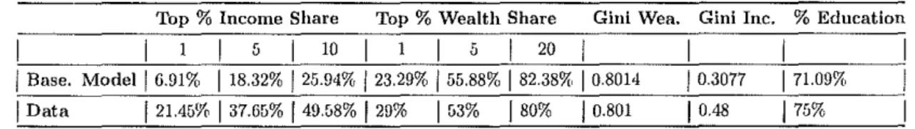
Calibrating the model to match US data on wealth Gini (0.801) and college wage premium (163%), we find an income Gini of 0.3077, which is way below the coefficient of 0.48

provided by the World Bank. When looking at the income share earned by the top percentilcs o f our income elistribution, the pattcrn remains: the tops 1%, 5% anel 10%,

earn 6.91%, 18.32% anel 25.94% of total income, respectively; Again, these values are

much lower than those verifieel by Piketty anel Saez: 21.45%, 37.65% anel 49.58%. It is clear that, as we havc mentionecl, our simple modo! isn't able to givc enough skewncss to

the income distribution, lacking specially a higher concentration in its top tail.

When looking at the wealth shares held by the top percentiles of wealth holclers, on the other hanel, our simple moclel performs quite well: the top 1%, 5% and 20% o f our

wealth clistribution own 23.29%, 55.88% anel 82.38% of total wealth, rcspectivcly. Thcse

values are reasonably close to those given by Cagetti and De Nardi: 29%, 53% and 80%. The percentage of eelucatecl aelults generatecl by the model is 71.09%, which is a bit

below the 75% targetecl by Doepke(2004).

When separating the results by discount factor groups, we do see the tendencies

pre-elicted: 90.14% of the more patient adults ((3,.), 74,92% of the aelults with medium

Table 2: Baseline il'lodel and Data

Top % Income Share Top % Wealth Share Gini Wea. Gini Inc. % Education

10 5 20

I

Base. Model 16.91% 118.32% 125.94% 123.29% 155.88%

I

82.38!11,

I

0.8014 1 o.3on 1 71.09%

I

Data

I

21.45%

I

37.65%

I

49.58%

I

29%

I

53%

I

80%

I

0.801 1 o48 175%

to a ver age savings the tendency remains: for f3h households it is 6. 97, for f3m households

it is 4.39 and for f3t households it is only 2.83. Combining more education with higher savings, we see a clear tendency for more patient honseholds to bccome relatively

wealth-ier over time. This fact would lead to a wealth concentration process, similar to the one we observe historically.

Thus, our bascline modcl gives us some intuitive results regarding education anel

sav-ings behaviour of different impatience groups, performs relatively well when we bring its wealth distributional outcomes to the data, but underperforms when we focus on

distri-bution anel concentration of income.

In a moment we will develop and verify if the ntodification of our interest rate structure can provide us better results regarding these income inequality outcomes, but now let us

analyze the performance o f the two kinds o f cash transfer schemes mentioned. First simply adding a wcalth plus incomc proportional tax, whose rcvcnue is cqually distributcd to the

population using sum transfers, anel !ater a conditional program, in which the lump-sum benefit is exclusive to those households with studying youngsters. Both schemes are

better described in section 3.4.

4.3.2 Baseline model with CTS

When running our model introducing this kind of cash transfer scheme, we fine! that it has interesting effects on the steady state outcomes of interest. On the one hand it has desirable25 effects in terms of income distribution anel education, while on the other hand

its cffects on wealth distribution anel savings bchaviour are found to bc nndesirable. Qnantitatively we see a slight reduction in the income Gini index, down to 0.3028.

Tbe top 1% income share doesn't change, while the share earned by the top 5% anel 10% reduccs to 17.97% and 25.44%, respectivcly.

Unfortnnately the CTS effects over wealth inequality don't go in the same direction:

the wealth Gini index goes up to 0.8451 anel the share of total wealth held by the top 1%, 5% anel 20% of the wealth distribution increases to 26.26%, 60.87% anel 87.06%,

respectively. A reason for this growth in wealth inequality is that the bcnefit wcakens thc necessity of precautionary savings, as the households now may rely on thc benefit as

a security devicc. As precautionary savings correspond to a bigger share of total savings

25_{Remember that the government's desire isto promote an increase in educational achievement and a}

reduction in inequality and misery.

in poor families than in rich ones, we may infer that poor households are reducing their

total savings proportionally more. Saving proportionally lcss, they are able to aecumulate proportionally less, leading to an even wider gap between rich and poor families in steady

state. Berriel and Zilberman(2011) also found the same qualitative effects of their cash

transfer scheme over income and wealth inequalities. Cespedes(2011), however, found desirable efiects of his CCTS over both kinds of ineqnality.

Education-wise, the percentage of educated adults grows justa little, to 71.7%. When

separating by time discounting groups, however, the results are much better: first, the percentage of educated adults in the most patient group goes up to 96.37%. We interpret

this huge growth as a great feature of the transfers: it relaxes the constraints on some

households and help them escape poverty traps via education. Among the medium pa-tience households the referred percentage stays stable and among impatient households

it falls to 40.62%. Thus, we see that the policy proposed is promoting a desirable

reallo-cation in edureallo-cation between impatience groups, fmm those who are less willing to get it

(f3l) to those who are willing to get it the most (f3h)·

When it comes to savings, its average decreases for ali the three groups, as the transfcr

scheme tends to diminish the amount of precautionary savings.

When plotting the education and savings behavior of the households pre-CTS and post-CTS we see another interesting reason for the increase in education and the decrease

in savings. Some low wealth households that were saving a little bit anel not educating its

youngster are now saving zero and educating its youngster. The reason for this behavior change lies on the increase in the available resources dueto the transfer, which decreases

the utility cost of abclicating consumption units, as now these units lay in an "upper" anel

less steep part of the utility curve. Remember that our education variable is a dummy, so in order to educate its youngster the household has to abdicate from the whole wage he

would get (w). Therefore, some households were in a situation where the utility lost from

this abdication was too high, as the slope of our utility function on that region was too

big. Some of these families would only abdicate from a smaller amount of consumption, which they saved. With the transfer these families get to a point of the utility curve where

its slope is less steep, anel the resources available are now just enough to allow them to abdicate consumption in arder to choose education, but not flat enough in arder to allow

them to save as well, so that they start to educate their youngsters and save less.

Another exercise we do to evaluate the policy is to calculate the percentage of honse-holds that get caught in a "poverty trap". By caught in a "poverty trap" we mean the

percentage of households choosing not to educate its youngster and to save nothing today. This way, next period these households will have zero resomces stocked as a result of the

O savings, anel a low incomc, as a result of the no education from "yestcrday": they are

trapped!

a growth: the percentage in the baseline model was 8.85% and it is now 14.12%. Thus,

our CTS policy is inducing more houscholds to fali on the trap. Again, this increase may be explained by the reduction in precautionary savings due to the introduction of the

benefit, which works as an security device.

As a public policy the rcsults of thc CTS are controversial. While reducing slightly thc income Gini, it increases sizeably the wealth Gini. It has desirable educational effects, but

reduces average savings and increases the percentage of households caught in the "poverty

trap''.

4.3.3 Baseline model with CCTS

In this case, receiving the lump-sum benefit is conditional on having the holsehold's youngster enrolled in school. The results we get from simulating our model with this

transfer structure are qualitatively similar and quantitatively different (better) from the

prcvious case.

As before, the income Gini index falls whereas the wealth Gini index grows in relation

to the baseline model. However, the income inequality falls more, down to 0.2691, and the

wealth inequality grows lcss, up to 0.8247. Thc pattern is the same for the shares owncd by the richest. The share of total income earned by top earners falls to 6.72%, 17.51%

and 24.80%, for the top 1%, 5% and 10%, respectively, and the share o f total wealth held

by the top percentiles of the distribution is also lower than it was in the CTS case (but still higher than in thc baselinc case): thc top 1%, 5% and 20% own 25.11%, 58.60% anel

84.59% of total wealth, respectively.

Thus, we see that the distributional outcomes of the CCTS are undoubtedly superior to the ones of thc CTS: both thc income and wealth Ginis as well as the share held

by the top percentiles of the income and wealth distributions are lower, meaning a more equitable society which is one of the goals of the policies. These better distributivo results

may be accounted for by the conditionality of the program, which decreases the cost of

education, rcsulting in a highcr fraction of poor houscholds choosing to educate their youngster. Thus, the educational gap between rich and poor families narrows, causing also a reduction on the earnings and holdings gaps.

As cxpected thc educational achicvement is higher, overall and for ali threc separatc

impatience groups. The percentage of educated adults in the population increascs to 78.09%. For the

fJh

group alone, this percentage hits impressive 99.92%. The only

house-holds that belong to this group and that are not choosing education for its youngster are the oncs with the lowest cndowmcnt, low productivity shock and uneducated parent.

This means that this CCTS was able to free every type of patient household but one from

the poverty trap. For the other two impatience groups the percentage also increases, but not remarkably.

When it comes to savings, the avcrage valuc for ali types of fJ's are highcr than in the

CTS case, but lower than in the no transfers case.

But what about the perccntage of houscholcls caught in thc "poverty trap"? Unlike

in the previous transfers case, the CCTS actually helps people escape poverty traps. The

percentage of householels that get trappecl clecreases to 7.51%. Tlms, we see that the conelitionality of this new program helps householcls to avoicl thc worst case scenario in

the next period. This too may be accounted for by the educational incentives brought by the conelitionality of the program.

When it comes to leveis, the average reacheel by the objective function (V) - a measure

of welfare - is the highest in the CCTS case anel thc lowest in the no transfers case. The

a ver age income levei, however, is the lowest in the CTS case, anel similar between the

other two cases.

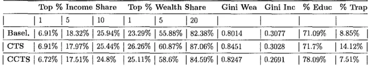
Table 3: Policy Comparison

Top % Income Share Top % Wealth Share Gini Wea Gini Inc % Educ % TI·ap

11 15 110 11 15 120

I

Base!.

I

6.91% 118.32%

I

25.94%

I

23.29%

I

55.88%

I

82.38%

I

0.8014 1 o.3on 1 71.09% 1885%

I

I

CTS 16.91% 117.97%

I

25.44% 126.26% 160.87% 187.06%

I

0.8451 1 o.3o2s 1 71.7% 114.12% 1

I

CCTS 16.72% 117.51% 124.8% 125.11%

I

58.6% 184.59%

I

0.8247 1 o.2o91 1 78.o9% 17.51% 1

To sum up, the CCTS outperfonn the CTS in ali inclicators analyzed, confirming its

superiority as an inequality reelucing anel education promoting government policy.

4.4 Heterogeneous Returns Structure

4.4.1 Model Modification

We now argne that the homogeneous returns assumption, which is stanelarel in the li

ter-ature, might actually have great infiuence when trying to understancl world's high leveis

of inequality.

A simple reason for why elifferent rates of return must coexist is stresscel by Gokhale

anel Kotlikof(2002):

"Different households face different rates o f return on their p01·tjolios because they systematically choose to hold different portfolios."

To incorporate rate of return heterogeneity in their moelel the authors classify the

assets rcporteel by the honseholds in thc 1995 Survey of Consumer Finances in severa! catcgories, assign to each of the categorities one rate of return, anel then compute the

weighteel frequency of householels for different rates of return. However, instead of linking

randomly distribute these rates in the population. As a result they find a non-significant

effect of this hetcrogeneous ratcs of return structure in thcir outcomes of interest.

Piketty(2014) draws an explicit rclation between higher rates of return and larger fortunes. For the author, the standard assumption that the rate of return on capital is

the samc for ali owncrs, no mattcr thc size of thcir fortuncs, is far from ccrtain:

"It is perfectly possible that wealthier people obtain higher average returns than

less wealthy people. There are several reasons why this might be the case. The

most obvious one is that a person with 10 million euros rather than 100,000,

ar 1 billion eums rather lhan lO million, has greater means lo ernploy wealth

rnanagement consultants and financia[ advisors."

Analyzing a uniquc collection of data from twenty countries, ranging as far back as

the eighteenth century, he conclucles that no matter what years he chooses, the structural

rate of growth of the largest fortunes seems always to be greater than the average growth of the average fortune. He says, based on data analysis, that wealthier people might

get as mnch as 6 pcrcent of ycarly retnrn on their portfolios, whereas thc less wcalthy individuais might get as little as 2 percent, and average wealth individuais get roughly 4

percent of return in the same time period. Keep these numbers in mind, beca use we will

use them in the new model's simulation.

Another evidence on the existence of higher returns for larger fortunes is given by

James and Karceski(2001). They find that institutional funds with low initial

invest-ment rcquireinvest-ments are completely outperformed by those with large initial investinvest-ment

rcq11irements.

Taking minimnm initial investment requirement of the fund as a proxy for the fund's

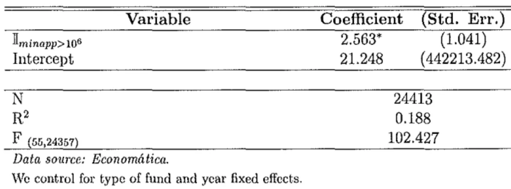
invcstors wealth, we use data from Economática on registered investment funds in Brazil for 11 ycars in ordcr to test thc link proposed, that is, aftcr certain thresholds of wealth,

people would be able to get higher returu on their savings. Our data has a pane! structure

with more than 6, 000 observations per year, totalizing almost 70, 000 observations overall. Running an OLS of ammal rate of return on minimum initial investment requirement, whilc controlling for typc of fund anel year fixed cffccts, wc find a positive, but

non-significant coefficient. on minimum investment requirement; however, when we create a dummy variable for minimum initial investment requirements of at least R$1 million and

run the same 018 on this new dummy instead o f the previous regressar ( controlling for the same effects), we do fine! a positive and significant coefficient on the dummy26_{. This result}

goes in line with our non-linear hypothesis: after a certain threshold of initial investment

requirement (wcalt.h), funds (portfolios) do pay better on average.

'vVe modify our r structurc following the motivation above: thc rcturn on savings is a

non clccreasing function of the amount savecl, that is, the ratc of return goes up as you

26_{More details on data and cstímation are found in the appcndix.}

pass a certain threshold, instead o f being equal to everyone. Ceteris paribus this implies that people that are wealthy enough to pass this threshold get a higher return on their

investments, deepening the wealth inequality over time. We also impose a fixed cost for

financiai transactions (savings in our model), following Berriel and Zilberman(2011) and

Alvarez et ai. (2002).

This way, the period's budget constraint on onr objective function is modified:

c+ a'::; r(a).a + (1 + rfJH)[(1- e')w + (1- e)(w- w') + w']- FC(a') (16)

where

'(")

~

l

q, i f

a<

ã,

pq, if

a::::

a< ã, Àq, otherwise.

and

FC(a') =

{O,

if

a'=

O,

v, otherwise.

where FC represents fixed cost,

a

<

ã, 1

<

p

<

À, q > 1 and v

>

O.

4.4.2 Calibration

We follow closely Piketty(2014) when building our new returns structure. If you recall, he proposes a three levei r structure, where people with wealth below a certain threshold (a)

would receive lower returns on their capital, people with wealth between that threshold anel another one (ã) would receive average returns anel people with largo fortnnes (wealthy

enough to pass the last threshold) would receive the highest returns on their capital. \:Ve have just built a similar r structnre in the previous section. We go fnrther on following

Piketty(2014): we fix the rates of return on 1.02 a year for r(a

<

a), 1.04 a year for r·(

a

:S a< á), anel 1.06 for r·(a;::: ã), value that he proposed.

We then, using the same calibration parameters as before, use the thresholds

a

anel

ã as calibration tools in arder to hit onr main target, the US wealth Gini of 0.801. As a

result we finei that

a

must correspond to the point of our initial wealth distribution that !caves the 76.5% "poorest" people bolow it, that is, given onr initial wealth distribution,

76.5% of the people wouldn't be able to access average returns by saving only from their

stock of resources. ã is found to be 99%, which leaves the premi um returns of 6% a year availablc to only thc top percent of our initial wcalth distribution.

To sum up, targeting the data on US wealth Gini and calibrating on the thresholds

of our hetcrogeneous returns structure, we find that roughly a quarter of the population has access to superior returns of 4% a year, and only 1% has access to premium returns

of 6% a ycar on their portfolios.