Conditional Treatment and Its Effect on
Recidivism
Herman J. Bierens
Pennsylvania State University, USA
& Tilburg University, The Netherlands
Jos´e R. Carvalho
∗Federal University of Ceara, Brazil
November, 2002
Abstract
The objective of this paper is to evaluate the effect of the 1985 ”Employment Services for Ex-Offenders” (ESEO) program on recidi-vism. Initially, the sample has been split randomly in a control group and a treatment group. However, the actual treatment (mainly be-ing job related counselbe-ing) only takes place conditional on findbe-ing a job, and not having been arrested, for those selected in the treatment group. We use a multiple proportional hazard model with unobserved heterogeneity for job seach and recidivism time which incorporates the conditional treatment effect. We find that the program helps to reduce criminal activity, contrary to the result of the previous analysis of this data set. This finding is important for crime prevention policy.
1
Motivation
During the period of 1980−1985, the National Institute of Justice (NIJ) sponsored a controlled experiment to evaluate the impact of reemployment
programs for recent released prisoners. Three well established programs were chosen, COERS in Boston, JOVE in San Diego and Safer Founda-tion in Chicago, to participate in the Employment Services for Ex-Offenders Program, henceforth ESEO. A total of 2,045 prisoners who voluntarily ac-cepted to participate were randomly assigned to either a treatment group or a control group. Those in the first group received, besides the normal ser-vices(orientation, screening, evaluation, support services, job development seminar, and job search coaching), special services which consisted of an as-signment to a follow-up specialist who provided support during the job search and the 180 days following job placement. The control group received only normal services. The inclusion of special services was a major response to the increasing belief that some past employment programs had failed because ex inmates lost contact with their original programs.
Using OLS regressions, Milkman (2001) found that the effect of the spe-cial services program is negligible. However, this evaluation of the ESEO program did not account for the the conditional feature of the treatment. The timing of the treatment was completely neglected and, as will be shown later, this is a very important characteristic of the program under evaluation
2
Characterizing the Program
2.1
Antecedents
During the last decades, sociologists and economists have been devising pro-grams to ease the difficult transition faced by ex-offenders during the period of time between release and reintegration into society. As experience has accumulated, a fundamental goal to a complete reintegration turned out to be job placement. A good job would be necessary not only to provide the basic needs for survival in the short run but also as a key element to secure self-esteem, security and sense of integration in the society as whole. Hence, sociological and economic theory have provided enough justification for the existence of employment services programs for ex-offenders.
effect on reducing criminal activity, unless for those who succeeded in secur-ing a job for a long time. These early results should not be interpreted as a failure but, in fact, should be viewed as just a first step to the design of bet-ter programs. The lack of follow-up afbet-ter placement was conjectured as the main obstacle to the complete success of such programs. As singled out by Mylkman, Timrots, Peyser, Toborg, Yezer, Carpenter, and Landson (1985):
“Historically, employment services programs have severed contact with the client immediately after job placement. If any follow-up occurs, it is usually limited to periodic telephone contact with the employer to determine if the client is still employed. The programs generally cease to provide support ... virtually abandoning him [client] during this crucial time in his adjustment to life outside of the institution.”
The new paradigm of employment services for ex-offenders have resulted in the appearance of programs that had a strong preoccupation with the post-placement of their clients. These programs have designed follow-up strategies to overcome the major criticism of past experience. Among various programs, three deserve recognition for both being successful and having similar struc-tures: the Comprehensive Offender Resource System, in Boston, the Safer Foundation, in Chicago and Project JOVE, in San Diego. Not surprisingly, the U.S. Department of Justice saw this as a opportunity for assessing the efficacy of employment services programs that contained a follow-up compo-nent. Then, in 1985 the Department of Justice funded a research performed by the Lazar Institute from McLean, VA. The next subsection describes the institutional details common to all three programs1.
2.2
Institutional Framework
There are four important institutional aspects in any employment program: the eligibility rule, the assignment (between controls and treatment) scheme, provision of treatment and outcome measurement. We postpone the two first aspects until Section 3, where the details about the available data set is discussed , since we believe to be a more appropriate place. Hence, in the ESEO program2, after being assigned to either the control or treatment
1
Of course, no program was identical to the others. However, specific attributes were not relevant to deserve separate analysis.
2
group3 the clients step inside the intake unit, where they received initial
orientation, screening and evaluation by an intake counsellor. While still in this first phase, to secure survival up to the job search phase, the intake counsellor offered minimal assistance services such as food, transportation, clothing and etc.
After intake, the client enters the second phase that will prepare him/her to develop job search skills: brief job development seminar which deals with issues like appropriate dress and deportment, typical job rules, goal setting, interviewing techniques, and job hunt strategy. It is assumed that the time spent in the first and second phases are not random and negligible compared to the search phase and the average duration of the outcome. The next and final phase of the provision of treatment is the job search assistance. This is the traditional job search assistance type of service, as described by Heck-man, Lalonde, and Smith (1999). The job search assistance is the stage in the ESEO program that is offered equally to both controls and treatments. The difference begins upon placement. Controls were not helped after placement whereas treatments started receiving follow-up help just after the employ-ment relation starts. The follow-up special services consisted basically of crisis intervention, counselling and, whenever necessary, reemployment assis-tance. These services lasted six months, and data from controls and treat-ments were collected at 30, 60 and 180 days after placement. For a more detailed exposition of each common service offered and received as well as those services specific of each individual program, one should consult Timrots (1985), Mylkman, Timrots, Peyser, Toborg, Yezer, Carpenter, and Landson (1985) and Milkman (2001).
3
The ESEO Program Data Set
The ESEO data set consist of of 2,045 individuals who participated in one of the three programs: 511 in Boston, 934 in Chicago and 600 in San Diego. However, the ICPSR4 only made available 1074 usable observations: 325 in
3
Unfortunately, there is know information whether clients knew their treatment status. As it will be clear later on, in the context of DT programs the state of knowledge about treatment status could help identified other parameters of interest besides the effect of treatment.
4
Boston, 489 in Chicago and 260 in San Diego. A large amount of information, sometimes very detailed, was collected from all sites. That can be broadly classified into three main categories:
• Background variables: demography, criminal history, employment history, educational achievement, and so on;
• Program variables: length of search, program participation record, reasons for drop-out, features of placement (wage, number of hours, match quality), and so on;
• Outcome variables: number of arrests, date of first arrest, self-reported arrests for placed people only, and so on.
A first important empirical issue is related to the characterization of the population being sampled. Unless very special assumptions are evoked, the validity of our findings can not be extrapolated beyond the population under sampling. In order to be eligible to participate in the ESEO program an individual must have the following background5:
1. Participants voluntarily accepted program services;
2. Participants had been incarcerated at an adult Federal, State, or local correctional facility for at least 3 months and had been released within 6 months of program participation;
3. Participants exhibited a pattern of income-producing offenses.
From the eligibility criteria it is clear that our population is a special, indeed very special, subset of the population of ex-offenders. Also, since partici-pation is voluntary and there is no information on non-participants (those who did not choose to participate even though they fulfilled requirements 2 and 3.), it is not possible to assess the potential bias on the sample induced by this selection scheme. Then, any result emerging from our econometric model must be interpreted considering those two initial issues. After this preliminary discussion, we should proceed analyzing the available sample.
5
Given the initial sample, the individuals were randomly assigned to either the treatment or control group. Controls receive the standard services and treatments received, in addition to that, emotional support and advocacy during the follow-up period of 180 days after placement. Two durations are of great importance, time spent searching a job and recidivism time. These two variables are grouped, however.
The point of departure for the choice of the covariates is Schmidt and Witte (1988): age at release, time served for the sample sentence, sex, edu-cation, marital status, race, drug use, supervision status, and dummies that characterize the type of recidivism. However, we also pay close attention to the criminologic literature in recidivism, for instance Gendreau, Little, and Goggin (1996).
The literature on unemployment (and job search) duration has been re-fined since the 70’s. Nowadays, it has a status of a complete theory of unemployment, as it appears in Pissarides (2000). Its empirical contents has been developed since the late 70’s and this first wave of empiricism is char-acterized for being concerned with “reduced” type models. A good account of this first phase can be found in Devine and Kiefer (1991). A final wave is characterized by advocating a “structural” approach to estimation and in-ference in such models. An updated account of that appears in van den Berg (1999). There has been also studies close to ours that try to measure the effect of programs in a context of a model of unemployment and job search duration. For instances, Abbring, van den Berg, and van Ours (1997), Eber-wein, Ham, and Lalonde (1997) and van den Berg, van der Klaauw, and van Ours (1998).
In view of those studies, a set of important covariates has been singled out. This set is composed basically of schooling, sex, age, and race. Together with the covariates related to recidivism, and the endogenous variables, the model variables are:
Endogenous variables
• ATTRITION: Indicator for attrition status. ATTRITION = 1 means the individual is either a “no show” or a “drop-out”, ATTRI-TION = 0 otherwise;
• SEARCH: Discrete variable indicating which interval6 the search
du-6
ration belongs to. SEARCH ={1,2,3 or 4};
• CRIME: Discrete variable indicating which interval7 the recidivism
belongs to. CRIME ={1,2,3,4 or 5 };
The search duration does not need any explanation, but the meaning of ”recidivism” is not unambiguous. There are two ways to measure recidivism outcomes in the ESEO program : through count data or duration data. Detailed data on the number of arrests from date of released to the end of the program for all clients was gathered in the respective state police departments. That was the data used in the original evaluation made by Mylkman, Timrots, Peyser, Toborg, Yezer, Carpenter, and Landson (1985). Also, data on the first arrest after release is available. The latter is what we will use as the duration of recidivism8. Thus, in the sequel ”(duration
of) recidivism” should be interpreted as the time between release and first rearrest.
Exogenous variables
• GROUP: Indicator for group participation. GROUP = 0 means control, GROUP = 1 means treatment;
• DRUG: Indicator for the use of drugs during the last 5 years. DRUG = 0 means no use, DRUG = 1 otherwise;
• RACE: Indicator for race. RACE = 0 means white, RACE = 1 means non-white;
• SEX: Indicator for sex. SEX = 0 means female, SEX = 1 means male;
• EDUC: Discrete variable describing educational attainment. EDUC = 0 if individual has from 2 to 8 years of schooling, EDUC = 1 if he/she has from 9 to 12 years or GED, and EDUC = 2 if he/she has more than 12 years;
7
See Appendix??.
8
• AGE: Age of ex-convict, in years;
• SANDIEGO: Indicator for city. SANDIEGO = 1 means San Diego, SANDIEGO = 0 means either Chicago or Boston;
• CHICAGO: Indicator for city. CHICAGO = 1 means Chicago, CHICAGO = 0 means either San Diego or Boston;
• AGEFIRST: Age at first arrest, in years.
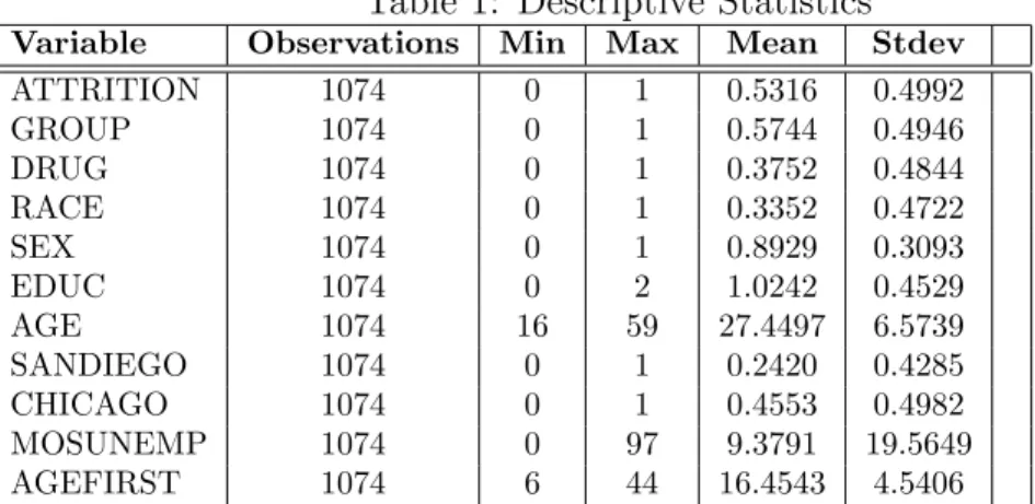
A summary of descriptive statistics of the covariates is given in Table 1.
Table 1: Descriptive Statistics
Variable Observations Min Max Mean Stdev
ATTRITION 1074 0 1 0.5316 0.4992
GROUP 1074 0 1 0.5744 0.4946
DRUG 1074 0 1 0.3752 0.4844
RACE 1074 0 1 0.3352 0.4722
SEX 1074 0 1 0.8929 0.3093
EDUC 1074 0 2 1.0242 0.4529
AGE 1074 16 59 27.4497 6.5739
SANDIEGO 1074 0 1 0.2420 0.4285 CHICAGO 1074 0 1 0.4553 0.4982 MOSUNEMP 1074 0 97 9.3791 19.5649 AGEFIRST 1074 6 44 16.4543 4.5406
4
An Econometric Model of the ESEO
Pro-gram
4.1
Identification of treatment effect
and den Berg (2000a) do not consider the presence of a control group as it is traditionally present in evaluation studies. Nevertheless, the treatment effect in our model is identified, but we have established this empirically rather than theoretically.
4.2
The Model
4.2.1 Absense of treatment
The latent dependent variables in or model are Ts,the job search time since
release from prison, and Tc, the time of the first arrest after release from
prison. Let V ∈ R+ be a random variable representing unobserved
hetero-geneity. In the absence of treatment the model could be specified according the approach advocated by van den Berg (2000): conditional on the unob-served heterogeneityV and the exogenous variables in a vectorX, the dura-tions Ts and are Tc independent. Adopting a proportional representation for
the hazard functions,
θs(t|X, V) =λs(t)·φs(X)·V. (1)
θc(t|X, V) =λc(t)·φc(X)·V. (2)
the conditional survival functions, given X and V, for each of the durations
Ts, Tc are
Ss(t|X, V) = P(Ts >t|X, V, W) = exp
µ
−V ·φs(X)·
Z t
0
λs(τ)dτ
(3)
Sc(t|X, V) = P(Tc >t|X, V, W) = exp
µ
−V ·φc(X)·
Z t
0
λc(τ)dτ
(4)
Hence, the joint conditional survival function conditional on X and V is:
S(ts, tc|X, V) = P [Ts≥ts, Tc ≥tc|X, V] (5)
= exp
µ
−V ·
µ
φs(X)·
Z ts
0
λs(τ)dτ +φc(X)·
Z tc
0
λc(τ)dτ
¶¶
Finally, in order tighten the durations Ts, Tc together and make them
out. Given a specification G(v) of the distribution function of V, the joint survival function conditional on X alone is:
S(ts, tc|X) = L
µ
φs(X)·
Z ts
0
λs(τ)dτ +φc(X)·
Z tc
0
λc(τ)dτ
,
where L(.) is the Laplace transform of G:
L(s) =
Z ∞
0
exp (−v.s)dG(v), s≥0.
4.2.2 Incorporating treatment
The key issue now is how to incorporate treatment in this framework. Let the dummy variableW represent group participation: W = 1 if the individual is selected in the treatment group, and W = 0 if selected in the control group. Then treatment is received if
1. The individual is selected in the treatment group: W = 1.
2. The job search has ended before the first arrest: Ts < Tc.
The problem is now that due to the latter condition it is impossible to build in the effect of treatment directly in the joint survival function (5) without sacrificing the conditional independence of Ts and Tc given X and
V. However, note that without assuming conditional independence we can still factorize out the joint density of Ts andTcconditional onX,V, andW,
as a product of conditional densities, say:
f(ts, tc|X, V, W)
= fc(tc|Ts =ts, X, V, W).fs(ts|X, V, W).
Consequently, the corresponding joint survival function can be written as
S(ts, tc|X, V, W)
= P [Tc≥tc, Ts ≥tsX, V, W]
=
Z ∞
ts
Z ∞
tc
Therefore, in modeling the joint survival function of Ts, Tcconditional onX,
V, and W we can still use a similar setup as before, as follows.
First, model the conditional hazard function of Tc conditional on Ts =
ts, X, V, W as
θc(t|ts, X, V, W)
= [(1−W)φc(X) +W.(1−I(t > ts))φc(X) +W.I(t > ts)φ
∗
c(X)]
×λc(tc)·V.
= [φc(X) +W.I(t > ts) (φ∗c(X)−φc(X))]×λc(tc)·V.
where I(.) is the indicator function. If W = 0 this specification corresponds to the previous one in (2), but for W = 1 the effect of the treatment on recidivism is now incorporated:
θc(tc|ts, ta, X, V, W = 1) =φ
∗
c(X)·λc(tc)·V if ts < tc
θc(tc|ts, ta, X, V, W = 1) =φc(X)·λc(tc)·V if not,
whereφc(X) is the same as in (2), andφ∗c(X) is the systematic hazard during
treatment. The corresponding conditional survival function of Tc is now
Sc(tc|ts, X, V, W) = P(Tc >tc|Ts=ts, X, V, W)
= exp (−V ·Λc(tc|ts, X, W))
where
Λc(tc|ts, X, W) (6)
= φc(X)
Z tc
0
λc(τ)dτ +W.(φ∗c(X)−φc(X))
Z tc
0
I(τ > ts)λc(τ)dτ
= φc(X)
Z tc
0
λc(τ)dτ +W.(φ
∗
c(X)−φc(X))I(tc> ts)
Z tc
ts
λc(τ)dτ
is the corresponding integrated hazard.
The conditional survival function of Ts is the same as before:
Ss(ts|X, V, W) = P(Ts >ts|X, V, W)
where
Λs(ts|X) =φs(X)
Z ts
0
λs(τ)dτ
is the integrated hazard. Thus, the joint survival function ofTs, Tcconditional
on X,V, andW is:
S(ts, tc|X, V, W) (7)
= P [Tc≥tc, Ts≥ts|X, V, W]
=
Z ∞
ts
Sc(tc|τ, X, V, W)fs(τ|X, V, W)dτ
=
Z ∞
ts
exp [−V ·Λc(tc|τ, X, W)]V exp (−V ·Λs(τ|X))φs(X)λs(τ)dτ
= V.φs(X)
Z ∞
ts
exp [−V ·(Λc(tc|τ, X, W) + Λs(τ|X))]λs(τ)dτ
where the last two equalities follows from
fs(t|X, V, W) = −
∂
∂tSs(t|X, V, W) (8)
= −∂
∂texp (−V ·Λs(t|X))
= V exp (−V ·Λs(t|X))φs(X)·λs(t)
4.2.3 Baseline hazards
The baseline hazards λs(t) and λc(t) are assumed to have a Weibull
specifi-cation:
λs(t) = λstλs
−1
, λs >0, (9)
λc(t) = λctλc
−1
, λc>0.
of the point of maximum of that parabolic hazards is close enough to the origin, the Weibull hazards is still a reasonable approximation. Then the integrated conditional hazards become
Λc(tc|ts, X, W = 1) (10)
= φc(X)tλcc+ (φ
∗
c(X)−φc(X))I(tc> ts)
¡
tλc c −tλ
c s
¢
and
Λs(t|X) = φs(X)·tλs. (11)
Hence, the joint conditional survival function for the treatment group takes the form:
S(ts, tc|X, V, W = 1) (12)
= I(tc> ts)V.φs(X) exp
¡
−V ·φc(X)tλcc
¢
×
Z tc
ts exp£
−V ·(φ∗
c(X)−φc(X))
¡
tλc c −τλ
c¢¤
×exp£
−V ·¡
φs(X)·τλs
¢¤
λsτλs
−1
dτ
+I(tc > ts) exp£−V ·¡φc(X)tλcc+φs(X)·tλcs
¢¤
+I(tc ≤ts) exp
£
−V ·¡
φc(X)tλcc+φs(X)·tsλs
¢¤
(see Appendix A for the details of the derivations involved), whereas for control group:
S(ts, tc|X, V, W = 0) (13)
= exp£
−V ·¡
φc(X)·tλcc +φs(X)·tλss
¢¤
4.2.4 Systematic hazards
For the systematic hazards φs(X) and φc(X) we adopt the usual
exponen-tional specification:
φs(X) = exp(βs′X), (14)
φc(X) = exp(β
′
where X contains 1 for the constant term. As to the specific hazard upon treatment, we assume that
φ∗
c(X) =δφc(X) =δexp(βc′X), δ >0.
In the sequel, however, we will continue to use the notations φs(X), φc(X)
and φ∗
c(X).
The parameter δ is the key parameter on our model, as it measures the effect of the ESEO program on the recidivism behavior of its participants. The parameter δ either inflates or deflates the systematic hazards function of recidivism upon placement. Its interpretation is:
• If δ > 1, the program has a negative impact on recidivism, as it in-flates the hazards for recidivism, therefore shortening the time between release and first arrest;
• If δ= 1, the program has no effect;
• Ifδ <1, the program has a positive impact on recidivism, as it deflates the hazards for recidivism, therefore lengthening the time between re-lease and first arrest.
4.2.5 Unobserved heterogeneity
The traditional9 choice of the distribution of the heterogeneity variable V
is the Gamma distribution, because its Laplace transform has a closed form expression: If V ∼Gamma(α, ω) then the Laplace transform of V is:
L(s) = E[exp(−s.V)] = (1 +s·ω)−α
, (15)
with derivative
L′
(s) =−E[V exp(−s.V)] = −αω(1 +s·ω)−α−1
. (16)
Adopting the specification it follows from (12) through (16) that:
9
S(ts, tc|X, W = 1) (17)
= I(tc> ts)αωφs(X)
×
Z tc
ts
£
1 +ω¡
φc(X)tλcc + (φ
∗
c(X)−φc(X))
¡
tλc c −τλ
c¢
+φs(X)·τλs
¢¤−(α+1)
×λsτλs
−1
dτ
+I(tc> ts)
£
1 +ω¡
φc(X)tλcc+φs(X)·tλcs
¢¤−α
+I(tc≤ts)
£
1 +ω¡
φc(X)tλcc +φs(X)·tsλs
¢¤−α
and
S(ts, tc|X, W = 0) =
£
1 +ω¡
φc(X)·tλcc +φs(X)·tλss
¢¤−α
. (18) Note that ω cannot be identified. To see this, substitute (14) in 18:
S(ts, tc|X, W = 0)
= £
1 + exp(ln(ω) +β′
cX)·tλ c
c + exp(ln(ω) +β
′
sX)·tλ s s
¤−α
.
Since X′
β1 and X′β2 contain constant terms, ln(ω) can be absorbed in the
constants. Consequently, we will set ω = 1.
4.2.6 Attrition
There are two times of attrition in our sample, namely “no show” if an individual does not participate at all in the job search stage of the program, and ”quitting” of an individual during the job search stage. As to attrition, we decided to take a very pragmatic approach. Instead of modelling these two types of attrition jointly with job search and recidivism, we assume that the survival functions (17) and (18) apply conditionallyon the absence of attrition, where attrition now includes ”no show” and ”quitting”.
If an individual quits after finding a job, and this individual is in the treatment group, we will assume that the treatment effect is the same as for an individual who completes the treatment.
Let A = 1 indicate attrition, and A = 0 absence of attrition. We will specify the probability of attrition as a Logit model:
P[A= 1|X, W =w] = 1 1 + exp (−γ′
wX)
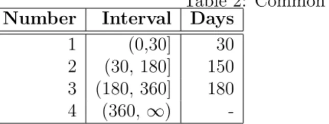
4.2.7 Censoring
The actual durationsTsandTcare not directly observed, but are only known
to belong to particular intervals, i.e., Ts and Tc are known to belong to one
of the following four intervals:
Table 2: Common Intervals
Number Interval Days
1 (0,30] 30 2 (30, 180] 150 3 (180, 360] 180 4 (360, ∞)
-There are 12 combinations where Ts and Tc are in different intervals:
Ts ∈[ai, bi), Tc∈ [ci, di), say, where either bi ≤ci or di ≤ai. The remaining
four cases, Ts∈[ai, bi), Tc∈[ai, bi), will be treated as ”other”, because there
are relatively few observations for which the latter applies, and secondly, the computation of P (Ts∈[ai, bi), Tc∈[ai, bi)) is more complicated than in the
non-overlapping cases.
Probabilities of the typeP(Ts∈[a, b), Tc ∈[c, d)) can easily be computed
on the basis of the joint survival functions:
P(Ts ∈ [a, b), Tc∈[c, d)|X, W) (20)
= S(a, b|X, W)−S(b, c|X, W) −S(a, d|X, W) +S(b, d|X, W).
4.3
The likelihood function
Let Ii = [ai, bi)×[ci, di), i = 1, ..., k, be disjoint intervals in R2+. For each
individual j, assign a dummy variable Di,j such thatDi,j = 1 if (Tc,j, Ts,j)∈
P[Di,j = 1|Xj, Wj] =P [(Tc,j, Ts,j)∈Ii|Xj, Wj]
= S(ai, bi|Xj, Wj)−S(bi, ci|Xj, Wj)
−S(ai, di|Xj, Wj) +S(bi, di|Xj, Wj)
= pi,j(θ),
say, where
θ= (β′
s, λs, β
′
c, λc, δ, α)
′
,
with Wj = 0 if individual j belongs to the control group, and Wj = 1 to the
treatment group. Moreover, the probability of an individual belonging to the category ”other” is:
P [D0,j = 1|Xj, Wj] = 1− k
X
i=1
pi,j(β) =p0,j(β),
say. Next, let Aj = 1 if individual j does not show up, or quit, with
proba-bility
P[Aj = 1|Xj, Wj =i] =qj(γi), i= 0,1
say. See (19). Moreover, recall that we have assumed that
P(Tc,j > a, Ts,j > b|Xj, Wj, Aj = 0) =S(a, b|Xj, Wj)
logL(θ, γ0, γ1)
=
n
X
j=1
Aj((1−Wj) lnqj(γ0) +Wjlnqj(γ1))
+
n
X
j=1
(1−Aj)
" k X
i=0
Di,jlnpi,j(θ) + (1−Wj) ln (1−qj(γ0)) +Wjln (1−qj(γ1)) #
=
n
X
j=1
Aj((1−Wj) lnqj(γ0) +Wjlnqj(γ1))
+
n
X
j=1
(1−Aj) [(1−Wj) ln (1−qj(γ0)) +Wjln (1−qj(γ1))]
+
n
X
j=1
(1−Aj) k
X
i=0
Di,jlnpi,j(θ)
= logL0(γ0) + logL1(γ1) + logL2(θ),
say, where n is the sample size.
4.4
Estimation and Inference
All econometric work (data manipulation, estimation and inference) was con-ducted by means of the econometric package EasyReg International10.
4.4.1 Attrition
Since we are going to estimate both vector of regressors γ0 and γ1
simulta-neously, we adjust the set of regressors X by way of the group dummy W. Hence, the actually estimated logit specification is:
P[N = 1|X, W] = 1 1 + exp (−X′
γ0−W ·X′(γ1−γ0))
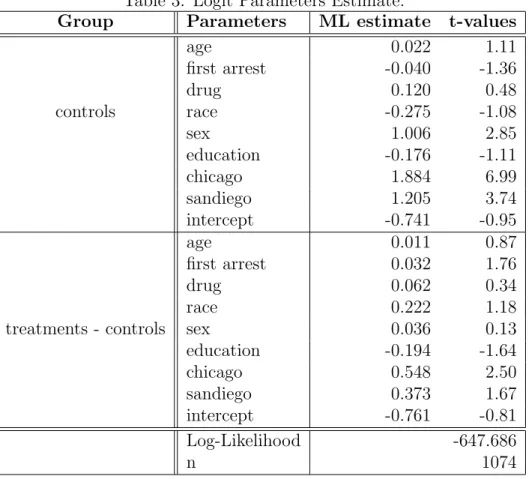
. (21) The results for the logit regression appear in Table 3. Note that given the logit specification, the second set of estimated parameters corresponds to
10
the difference between the estimated parameters of treatments and controls. Thus, the first set of estimates are the estimates of the components of γ0,
and the second set corresponds to γ1 −γ0. The majority of the estimated
regressors are not significant at the 10% level11.
Table 3: Logit Parameters Estimate:
Group Parameters ML estimate t-values
age 0.022 1.11
first arrest -0.040 -1.36
drug 0.120 0.48
controls race -0.275 -1.08
sex 1.006 2.85
education -0.176 -1.11
chicago 1.884 6.99
sandiego 1.205 3.74
intercept -0.741 -0.95
age 0.011 0.87
first arrest 0.032 1.76
drug 0.062 0.34
race 0.222 1.18
treatments - controls sex 0.036 0.13 education -0.194 -1.64
chicago 0.548 2.50
sandiego 0.373 1.67
intercept -0.761 -0.81 Log-Likelihood -647.686
n 1074
For controls, only variables sex, chicago and sandiego are significant. A man has a higher probability of attrition than a woman. Belonging to the program located in Chicago, as well as in San Diego, raises the probability of attrition. Most of the components of γ1 −γ0 are insignificant, except the
dummy Chicago: for ex-inmates having served their last term in a Chicago
11
prison, the probability of attrition is higher for the treatment group than for the control group.
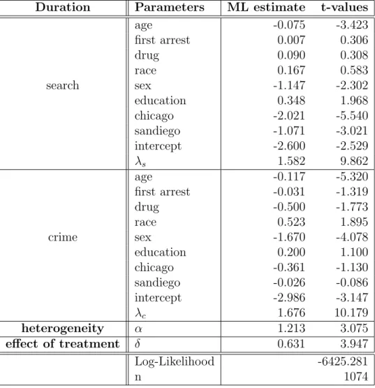
4.4.2 Job search, recidivism, and treatment
Results appear in table 4. In order to interpret the results, note that if a coefficient is positive and the corresponding X variable increases, then the whole hazards function will be inflated, hence the integrated hazard will be reduced, and so will be the survival probability. Thus, failure will occur earlier. In the case of search duration, this implies that the average time of search (unemployment) will be lower the higher the value of the X variable is. For the crime (recidivism) duration this implies that the expected time between release and rearrest will be reduced.
Some parameter estimation results for search duration appear to con-tradict well established facts in the literature of empirical search models. However, given the specific nature of our data (ex-criminals), there are some reasonable explanations for that. The demand side of the job market appears to be driven much more by the possibility that the future worker could com-mit a crime after being hired than by pure efficiency considerations. Also, the job market for ex-criminals is characterized by being of bad quality and by offering low wages. Such empirical evidence concerning job search for ex-inmates looks promising as a topic for future development.
The estimated parameter for age is negative and therefore, as expected, the job search time is higher the older the ex-inmate is.
Males appears to have search time greater than the search time of women. This is the first result that contradicts empirical findings in search models. Indeed, the sex effect is significant. However, the male/female ratio of in-mates is much higher than the 50% ratio out of prisons, so that males may present a higher potential threat of comitting a crime while employed. The positive coefficient of education means that more educated ex-inmates will find jobs faster than less educated, which is in accordance with the empirical search literature. See, e.g., Devine and Kiefer (1991). The significantly neg-ative coefficients of the dummies for Chicago and San Diego, indicate that job search time in Chicago and San Diego12 larger than in Boston, ceteris
paribus. Finally, the parameter of the baseline hazards presents a rather surprising result. As shown in Lancaster (1990), a value of λs= 1.582 means
12
Table 4: Parameters Estimate:
Duration Parameters ML estimate t-values
age -0.075 -3.423
first arrest 0.007 0.306
drug 0.090 0.308
race 0.167 0.583
search sex -1.147 -2.302
education 0.348 1.968
chicago -2.021 -5.540
sandiego -1.071 -3.021 intercept -2.600 -2.529
λs 1.582 9.862
age -0.117 -5.320
first arrest -0.031 -1.319
drug -0.500 -1.773
race 0.523 1.895
crime sex -1.670 -4.078
education 0.200 1.100
chicago -0.361 -1.130
sandiego -0.026 -0.086 intercept -2.986 -3.147
λc 1.676 10.179
heterogeneity α 1.213 3.075
effect of treatment δ 0.631 3.947
Log-Likelihood -6425.281
n 1074
that the search time presents positive dependence, or in other words, the longer an individual keep searching the higher the probability of finding a job. This is exactly the opposite of a lot of evidence found in studies of search in the labor market. For instance, see Devine and Kiefer (1991). A plausible explanation for the high value of λs (which is significantly greater
(low-paying) job that becomes available.
The impact of age on the expected recidivism time is significantly nega-tive.This is in accordance with other studies in recidivism such as Schmidt and Witte (1988). Hence, ceteris paribus, an older ex-inmate will postpone his/her next crime. The estimated parameter of the dummy variable race (1 = black) is positive, but only borderline significant. Hence, non-whites seem to recidivate earlier than whites, which is in accordance with other empiri-cal studies on recidivism, such as Schmidt and Witte (1988). The strongly significant negative value of the coeffient of sex appears to contradict the literature on criminal recidivism: females will commit a crime earlier than males. However, the sample consists only for about 11% of females, so that a very few bad ones among them may cause this effect. The city dummies do not have a significant effect. Also for recidivism the parameter λc is
sig-nificantly greater than 1, which implies that the longer an ex-inmate is out without committing a crime the higher the probability of committing a crime in the future.
The parameter α is a nuisance parameter with no particular interesting interpretation other than that it is the expected value of the unobserved heterogeneity variable V.
The parameter δ is the key parameter on our econometric model. The estimated value is significantly less than 1.Hence, the program is effective
as it increases the time between release and rearrest. This result stands in contrast with the original study of the ESEO program, as shown in Mylkman, Timrots, Peyser, Toborg, Yezer, Carpenter, and Landson (1985).
5
Conclusion
By modelling the ESEO program as a mixed multivariate proportional haz-ards model13, where treatment is conditional on placement, we have merged
two important fields of modern econometrics: survival analysis and econo-metric evaluation of programs. As far as we know, our paper is the first one to build this type of model and estimate it. The following paragraphs conclude by discussing the main achievements of the present paper, as well as by offering some possible ideas for future research.
First, our contribution has to do with the available data set. Even though this data set has been used before, it was restricted to the community of
13
sociologists and criminologists. Despite the fact that search models have been estimated since the early 80’s, search by ex-inmates who participate in a program of reemployment is a novelty for the econometric audience. The estimated parameters appearing in table 4, and the discussions that followed it show that some regressors have very different effects when compared to the traditional search model. Nonetheless, our available data presents some limitations. The main limitation of our data set is that it is grouped and this definitely imposes constraint on what can be identified from the model and makes our results less convincing. A good standard to be followed by criminologists and sociologist would be the methodology used by the agencies that collect unemployment data in the USA. Better data help a lot, specially in econometric evaluation of programs, as shown by Heckman, Lalonde, and Smith (1999).
Second, we have shown some evidence of how the process of search for jobs could be heavily influenced by the demand side of the market. More specifically, it would not be surprisingly that information asymmetries play a crucial role in this specific labor market. It is very likely that all prospective employers know that each of application comes from an ex-inmate, however knowledge of the past criminal history of each ex-convicts does not need to follow. Indeed, legislation regarding disclosure of criminal past records varies a lot within the USA. Hence, an interesting topic for future research would be estimation of models that explicitly consider the information asymmetries existent in this market. We think this should be a nice starting point to address the actual debate about disclosure of criminal records and to evaluate its policy implications.
Third, the blending of survival analysis and econometric program evalu-ation represents our key contribution. We have set a model where the timing of treatment is explicitly considered. This stands in contrast with any other past study of econometric evaluation of programs. In fact, we are able to build an estimable model and estimate it. The estimated parameters clearly show that the timing of treatment is an important feature of social programs well neglected in the past. Nonetheless these initial accomplishments, there is still important topics for future development. Although the parameter δ
and this should be accounted for.
This lead us to suggest an urgent new avenue to explore: build models that assume impact heterogeneity. From the perspective of our model this means to specify the following:
δ(X) =J(X) where J(X)≥0 for all X ∈Rn. (22) Thus, the effect of the program is conditional on a set of regressors represent-ing individual-specific, program-specific and local variables. Undoubtedly, this would give us a much more accurate picture of the program. As a mat-ter of fact, an easy choice would beδ(X) = exp[X′
β]. However, identification of the model becomes a problem!
APPENDIX
A
Joint Survival Function
It follows from equations (7), (10) and (11) that:
S(ts, tc|X, V, W = 1) (23)
= V.φs(X) exp
¡
−V ·φc(X)tλcc
¢
×
Z ∞
ts
exp£
−V ·(φ∗
c(X)−φc(X))I(tc> τ)
¡
tλc c −τλ
c¢¤
×exp£
−V ·¡
φs(X)·τλs
¢¤
λsτλs
−1
dτ
= I(tc> ts)V.φs(X) exp
¡
−V ·φc(X)tλcc
¢
×
Z ∞
ts
exp£
−V ·(φ∗
c(X)−φc(X))I(tc> τ)
¡
tλc c −τλ
c¢¤
×exp£
−V ·¡
φs(X)·τλs
¢¤
λsτλs
−1
dτ
+I(tc≤ts)V.φs(X) exp
¡
−V ·φc(X)tλcc
¢
×
Z ∞
ts
exp£
−V ·¡
φs(X)·τλs
¢¤
λsτλs
−1
dτ
= I(tc> ts)V.φs(X) exp
¡
−V ·φc(X)tλcc
¢
×
Z ∞
0
I(τ > ts) exp
£
−V ·(φ∗
c(X)−φc(X))I(τ < tc)
¡
tλc c −τλ
c¢¤
×exp£
−V ·¡
φs(X)·τλs
¢¤
λsτλs
−1
dτ
+I(tc≤ts) exp
£
−V ·¡
φc(X)tλcc +φs(X)·tsλs
¢¤
= I(tc> ts)V.φs(X) exp
¡
−V ·φc(X)tλcc
¢
×
Z ∞
0
I(ts < τ < tc) exp
£
−V ·(φ∗
c(X)−φc(X))
¡
tλc c −τλ
c¢¤
×exp£
−V ·¡
φs(X)·τλs
¢¤
λsτλs
−1
dτ
+I(tc> ts) exp
£
−V ·¡
φc(X)tλcc+φs(X)·tλcs
¢¤
+I(tc≤ts) exp
£
−V ·¡
φc(X)tλcc +φs(X)·tsλs
¢¤
S(ts, tc|X, V, W = 0) (24)
= exp£
−V ·¡
φc(X)·tλcc +φs(X)·tλss
¢¤
The integral in (23) can be further “simplified” as:
Z ∞
0
I(tλs s < τλ
s
< tλs c )
×h1 +ω³φc(X)tλcc+ (φ
∗
c(X)−φc(X))
³
tλc c −
¡
τλs¢λc/λs
´
+φs(X)·τλs
´i−(α+1)
dτλs
=
Z ∞
0
I(tλs
s < u < tλ s c )
×h1 +ω(φ∗
c(X)−φc(X))
³ ¡
tλs c
¢λc/λs
−uλc/λs
´
+ωφs(X)·u
i−(α+1)
du
=
Z q
p
£
1 +ωφc(X)tλcc +ω(φ
∗
c(X)−φc(X)) (qr−ur) +ωφs(X)·u
¤−(α+1)
du
= 1
a[ωφs(X)]
−(α+1)
Z q
p
a[b+x+c(qr−xr)]−(a+1)
dx
say, where
a = α
b = 1 +ωφc(X)t
λc c
ωφs(X)
c = φ ∗
c(X)−φc(X)
φs(X)
p = tλs s
q = tλs c
r = λc/λs
Finally, note that in order for the integral14
Z q
p
a[b+x+c(qr−xr)]−(a+1)
dx (25)
14
to be well-defined, we must require that:
a >0, b≥0, p≥0, q ≥p, r ≥0, and c >− b+p
qr−pr. (26)
References
Abbring, J., and G. V. den Berg (2000a): “The Non-Parametric Iden-tification of Treatment Effects in Duration Analysis,” Unpublished Paper, Free University of Amsterdan.
Abbring, J., G. van den Berg, and J. van Ours (1997): “The Ef-fect of Unemployment Insurance Sanctions on the Transition Rate from Unemployment to Employment,” Working Paper, Tibergen Institute.
Abbring, J. H., and G. V. den Berg (2000b): “The Non-Parametric Identification of the Mixed Proportional Hazards Competing Risks Model,” Manuscript, Free University of Amsterdam.
Beck, A. J., andB. E. Shipley(1989): “Recidivism of Prisoners Released in 1983,” Special report, Bureau of Justice Statistics.
Devine, T., and N. Kiefer (1991): Empirical Labor Economics: The Search Approach. Oxford University Press, New York.
Eberwein, C., J. Ham, and R. Lalonde (1997): “The Impact of Being Offered and Receiving Classroom Training on the Employment Histories of Disadvantaged Women: Evidence from Experimental Data,”Review of Economic Studies, 64, 655 – 682.
Gendreau, P., T. Little, and C. Goggin (1996): “A Meta-Analysis of the Predictors of Adult Ofender Recidivism: What Works!,”Criminology, 34(4), 575 – 607.
Heckman, J., R. J. Lalonde, and J. A. Smith(1999): The Economics and Econometrics of Active Labor Market Programsvol. 3A ofHandbook of Labor Economics, chap. 31, pp. 1865–2097. Elsevier Science, Amsterdan.
Maltz, M. D. (1984): Recidivism, Quantitative Studies in Social Sciences. Academic Press, Orlando, FL.
Milkman, R. (2001): “Employment Services for Ex-Offenders, 1981-1984: Boston, Chicago, and San Diego,” Discussion Paper 8619, ICPSR.
Mylkman, R., A. Timrots, A. Peyser, M. Toborg, B. G. A. Yezer, L. Carpenter, andN. Landson(1985): “Employment Services for Ex-Offenders Field Test,” Discussion paper, The Lazar Institute.
Pissarides, C. A. (2000): Equilibrium Unemployment Theory. The MIT Press, Cambridge, MA, second edn.
Schmidt, P., and A. D. Witte (1988): Predicting Recidivism Using Sur-vival Models, Research in Criminology. Springer-Verlag.
Timrots, A.(1985): “An Evaluation of Employment Services Programs for Ex-Offenders,” Master’s thesis, University of Maryland, College Park.
van den Berg, G. (1999): “Empirical Inference with Equilibrium Search Models of the Labor Market,” The Economic Journal, pp. F283 – F306.
(2000): Duration Models: Specification, Identification, and Multiple Durationsvol. V ofHandbook of Econometrics. North Holland, Amsterdam.
van den Berg, G., M. Lindeboom, and G. Ridder (1994): “Attrition in Longitudinal Panel Data and the Empirical Analysis of Dynamic Labour Market Behavior,”Journal of Applied Econometrics, 9, 421–435.