Barriers to trade: barriers to growth

•

ｾ＠ ... FUNDAÇÃO ... GETULIO VARGAS EPGE

Escola de Pós-Graduação em Economia

"BARBIEBS TO

rBADE: BARBIEBS TO

GBOWTH."

PEDRO CAVALCANTI FERREIRA

(EPGE/FGV)

LOCAL

Fundação Getulio Vargas

Praia de Botafogo, 190 - 10° andar - Auditório

DATA

23/10/97 (sa feira)

HORÁRIO

16:00h

•

..

..

Barriers to nade: Barriers to Growth*

Pedro Cavalcanti Ferreira

EPGE - Fundaçao Getulio Vargas

Alberto Trejos

Northwestern University

May 20, 1997

Abstract

We study the cxtent to which differences in international trade policies contribute to the significant cross-country disparities in macro-economic performance. In particular, wc concentrate on the effect of protectionism on generating differences in leveIs (of income and of measured total factor productivity), in growth rates (of output, productivity and inputs), in volatility and in trends (or development traps). We document that these rclationships are strong in cross coun-try data, integrate a Hecksher-Ohlin mode! of international trade into the standard macroeconomic modcl to derive those rclationships an-alytically, and to quantify them. Our results suggest that a large fraction of the cros::; country variations can be attributed to trade policy.

1

Introduction

•

which differences in institutions and national policies (rather than in more permanent. idiosyncratic fundamentaIs) can be the reason why some coun-tries are rich and others are poor. some grow fast and others grow slow. some are volatile and others are stable. etc.l _{In this paper. we join those efforts}

and ask whether much of the disparity in macroeconomic performance can be attributed to differences in tariffs and other international trade policies. It is our belief that for many countries. the large degree of protectionism carries a good part of the blame for their disappointing macroeconomic performance. The notion that trade policy affects macroeconomic variables significantly is. of course. not new. At least in Latin America. this ide a is an integral part of the policy debate. There is abundant empirical support for the notion that protectionism is behind the disappointing performances of many countries.2

AIso, one cannot help but notice that the four South East Asian ;;dragons," happen to be among the Third vVorld countries that trade most intensively with the rest of the world. We study here if the simplest open-economy macroeconomic model can deliver the most salient qualitative features of the data. Then, using standard procedures to discipline our choice of pa-rameters, we quantify the importance of the link between trade policy and macroeconomic performance.

We provide below some illustration of the strong correlations between trade policy and economic performance that can be found in the data. Those relationships, while strong, do not imply causality. There are good static, mi-croeconomic reasons why a country is better off without protectionist trade policies. A government or a set of institutions that can pick the right macro-economic policy (and thus get high leveIs of productivity and growth rates) is more likely to be able to pick the right international trade policy (and thus select low tariffs and eliminate non-tariff trade restrictions), even if those two sets of policies have nothing to do with one another. To understand if the relationships are not coincidence. one needs a macroeconomic model with international trade, to study which channels establish the link between trade and macroeconomic performance within the model, and then use the data to evaluate the quantitative importance of those channels. That is what we do.

1 For example, Chari, McGrattan and Kehoe (1996) show how differences in income

leveIs could respond to differences in the leveI and trend of capital taxes. Parente and Prescott (1996) study how the protection of monopolies can generate "technological bar-riers" that multiply the differences in total factor productivity. Rebelo (1991) shows how fiscal polic)' can affect long-run growth.

•

..

To pursue this. we integrate a static Hecksher-Oh1in model of interna-tional trade into the standard Cass-Koopmans macroeconomic model. As in Trejos (1992) and Ventura (199<-1). the way this is done is by allowing for the existence of tradable and non-storable intermediate goods. which are used in the production of a non-tradable final good. These intermediate goods are produced with different factors than the final good. As a consequence, one can solve this model sequentially. The problem of factor alIocation and trade in intermediate goods is static: one can then treat the solution to this problem as an implicit technology. and the dynamic problem becomes homeomorphic to a one-good optimal growth model. To distinguish between permanent differences and differences along transition paths. the model is designed so that, if alI countries are identical except for their trade policies, an economy in autarchy and an economy with completely free-trade would have the same steady state.

The main results are as folIows. First. we show that there is a clear pos-itive correlation between the total factor productivity of nations and their openness to trade: our model delivers that correlation. as in it gains from trade show up in output rather than in consumption. Quantifying the model we find that for the median country 1/6 of TFP differences with respect to the US can be attributed to different trade policies: for some countries with extremely high tariffs. it is 1/2 of TFP differences. Second, we show that there is a clear positive correlation between the growth rate (in inputs, productivity and output) of nations and their openness to trade: our model delivers those correlations: it predicts that changes in trade polic)' are corre-lated with TFP growth and that, because trade affects the marginal returns to capital. leveIs in trade policy are correlated with inputs growth. Quan-tifying the model we find that. for some countries, changes in trade policy between 1970 and 1985 have generated TFP gains or losses of as much as 10% of total output. and that such channel has been more important than human capital accumulation: also, for the average country, in that period the difference between a very open and a very closed trade policy would amount to as much as 5% more input growth and 12% more output growth, and for a quarter of the world economies those numbers would be 15% and 24%.

•

..

also delivers that resulto as under high tariffs the distortions in the ecanomy generate a non-convexity. that allows there to be a second, stable state at a lower leveI of inputs than the free-trade steady state. Quantifying the model we find that this ;;development trap" exists, at our baseline parameters. for effective protection rates of about 50% or over: at the trapo depending af the tariff rate. the income leveI may be 10% to 25% of the free-trade steady state income level.

In Section 2 we present the model and the solution method. and also dis-cuss the data that we use. Section 3 then addresses the topic af cross-country differences in leveIs of output and of measured total fador productivity. FirsL we document the extent of those differences, and how they relate to trade policy. Then, we show how and why our model predicts a qualitatively similar pattern as the one displayed in the data. Finally, we quantify the model to assess the importance of the relationship between output leveIs and trade policies, and compare it with the quantitative importance displayed in the data. In Section 4, we look at the topic of cross-country differences in growth rates (of inputs, productivity and output). The analysis follows the same order outlined before: first we look at the data, then study the model analytically, and finally quantify the results. The same is done in Sec-tion 5, where we study cross-country differences in trends and the apparent occurrence of "development traps.·· In Section 6 we summarize and conclude.

2 The IDadel

Time is discrete and unbounded. Our representative country is small. and populated by a continuum of identical. infinitely-lived individuaIs. There are three goods produced in this economy. Two of those goods, called A and B, are non-storable intermediate products. and can be traded with the rest of the world (at a relative price denoted p: from the point of view of our small

economy p is taken as given, and we provide details about its determination and law-of-motion below). The other good. called Y, is a final good that can be consumed or invested, but that cannot be traded. There are also three factors of production in this economy, inelastically supplied: raw labor (denoted L, and growing at a constant rate f-l due to population growth and exogenous. labor-augmenting technological progress), human capital (H) and physical capital (K).

the production of the intermediate goods A and B, with constant returns technologies. For now. we assume that this technologies are Cobb-Douglas: most of the theoretical results only require homogeneity of degree one:

A - h-Ua L l-ua

.-1. A B T. -na L l-Ub

- ICB B .

vVithout loss of generality, we assume that A is the labor-intensive good. that is. na

<

nb·

The production of the final good Y utilizes the intermediate goods as weU as human capital. Denoting by a and b the amounts used of intermediate

goods (since these are tradable, it is possible that a

=I

A or b

=I

B), it obtains

that

(1)

Notice that we have assumed. at the cost of some generality, that those factors used in intermediate goods production cannot be used in final good production; this will simplify matters very significantly, as will be seen below. Final goods can be used in either consumption C or investment (in phys-ical capitaL IK : or in human capital IH), and cannot be stored. The process

by which these investments show up in next-periods capital is not a linear accumulation function, as investment is a convex technology and existing capital facilitates accumulation:

(

K 1-1>

K' = (1 - 8)K

+ r

I

K ) IK .

(2)

This type of law-of-motion is emulated from Lucas-Prescott (1971) and oth-ers, and in our model delivers a better calibration than the standard law-of-motion. Notice that a higher K would facilitate investment. but K does not appear in (2) as an input. For human capital. we wiU try two alternative formulations, detailed in Section 4. In the first formulation, we just give H a law of motion identical to (2); in the second formulation, we assume that the human capital is embedded in the acquisition of physical capital. so whenever one invests in a unit of K one also acquires one unit of H.

•

assume that the government chooses a fiat. ad-valorem tariff r: the proceeds of that tariff are transferred back to the households.

The world contain man)' countries. all with identical preferences and tech-nologies. although with different trade policies.3 _{All but one of those}

coun-tries are small. in the sense that they also take the international price p as

given. There is one large country. whose domestic shadmv price of A in terms of B becomes the international price p: it has tariffs r = O. and has been around for long enough to have converged to its stochastic balanced growth path. When calibrating the model. we \vill pick data to make that large economy resemble the U nited States.

2.1

Solution of the model

Notice that the allocation of capital K and labor L among the production of the intermediate goods

A

and

B

is a purely static problem: this because the two intermediate goods are not ｳｴｯｲ｡｢ｬ･ｾ＠ there is trade balance in every period. and the factors used in the production of A and B have no other use. Similarly. the amounts used of those intermediate ｰｲｯ､ｵ｣ｴｳｾ＠ a and b, are also

determined in a static problem. Consequently, one can solve the model in two steps: first. one can obtain the equilibrium quantities (A, B, a, b) as functions

of (K, L, r, p). and derive an equilibrium mapping Y = F(K, H, Llr, p) by substituting those equilibrium quantities into (1). Second, one can use that equilibrium mapping

F

as if it was an exogenously given technology, and solve the standard dynamic problem that emerges as a resulto

To derive the mapping F, notice that K and L are allocated in a way that maximizes the domestic value of intermediate good production:

A,B - argmaxqA

+

B A.B

s.t.A

<

KOt.a L1-Ot.a

A A B

<

KOt.a L1-Ot.b

B B

KA+KB

<

K

LA+L B

<

L

3Whcn talking about total factor productivitic:;. wc will intcrprct thcm a:; if all thc

•

..

Similarly. the input of intermediate goods in to the final good sector satisfies

a. b arg ma"\: a -y b1--y

a.b

s.t.qA.

+

B

>

qa

+

b

and the two problems are linked by the current account balance pa

+

b

=

pA

+

B. The local prices satisfy q = p/ (1

+

7) if the country is

labor-abundant (if K / L

<

K* / L

*,

where K* and L * are the leveIs available in the large foreign economy described above): q = p(l

+

7) if K/ L

>

K* / L*.

The allocation of K and L between the sectors A and B will ma'{Ímize the value of total tradables outpuL under local prices q. This means that in

equilibrium

o kCta_- 1 a a

ｯ｢ｫｾ｢Ｍｬ＠

ivJRTsA = q

(1 - ｯ｡Ｉｫｾ｡＠

- (1 - Ob) ｫｾ｢＠ = q.

The demand for a and b will satisfy

,b

MRTSba = q or (l-,)a = q.

It can be shown that there is a tariff rate T, which depends on K/ L, such that if 7

2:

T international trade shuts down and the equilibrium is autarchic ..

When 7

2:

T one can represent the map F as the solution for the planning

problem for an economy that cannot trade. Conveniently, this takes also the form of a Cobb-Douglas technology, namely

where

a

= ,Oa

+

(1 -,)Ob and

n

is a function of parameters.

Under free trade (7

=

O). there is a criticaI leveI k* such that:

1. If k

<

k* the country exports A. the labor-intensive good: 2. If k

>

k* the country exports B, the capital-intensive good:

•

..

The capital-labor ratio k'" is a function of p. which would be the price of A

in a closed economy that had caPital-labor ｲ｡ｴｩｾ＠ k*. Therefore. ak* / ap >

o.

AIso. there are critical leveIs k.-4. < k* and kB

>

k*. also functions of p.

such that:

1. If k

<

k_A then the country only produces A;

2. If k

>

k_B then the country only produces B.

With a positive but ;;smalr tarif[ there is an interval ｛ｫｾＬ＠ k

_2]

ｾ＠ containing

k*, such that if k E ｛ｫｾＬ＠ k

_2]

the econ0T-Y does not trade.

akU a7

<

O, and lim ｫｾ＠ = lim k.4. = O. Analogous statements can be

'7--+00 T--+OC

made for k

2

and k B·

Recall that what matters for production is the equilibrium value

If the economy trades freely (7 = O) then

g(K,Llr

= O,p) = {

If 7

>

O but 7

<

x then

[hKCta Ll-Cta

if

K/ L

<

k

_A

fhK

+

n4L

if

K/ L

E

[k

A ,

kB]

n

₅

K CthL

1

_{-Cl:b ifK/L>kB}

n

₆

KCta U-Cl:a

if

K/ L

<

k

A

n7K

+

nsL

if

K/ L

E

[k

A , ｫｾ｝＠

g(K,LI7,p)

= nlKliL1-1i if

K/L

E ｛ｫｾＬｫＲ｝＠

ngK

+

nlOL

if

K/ L

E

[k

_2,

kBl

nllKCl:h U-Cl:b

if

K/ L

>

_kB

The values

n

i are functions of parameters; most are affected by p and 7. (3)

Consider for starters the dynamic problem of an economy facing constant prices p and constant tariffs 7, taken as given. From the point of view of that

dynamic problem, the production function

F(K,H,L)

=

g(K,LI7,p)O'H

1-0'

- - - ---- - - --- -

-..

..

Lenuna 1 The implicit production function F is continuous, and

homoge-neous of degree one. For r

=

O and for r

=

x, F is also Cl and strictly

concave. Concavity, and continuity of the first derivative, are generic but not

global properlies of F if r E (O, r). In parlicular,

F(K, H, Llr,p) = g(K/ Llr,pt'(H/

L)l-a-and the function g(klr, p) is increasing L)l-a-and continuous in k, but there is a finite number of values of k for which g' (k) has a discrete variation (up or

down).

For all values of p, there is a level of K/ L (call it K(p)) such that F 2S

invariant in r; for all other values of K/ L#- K(p), F is decreasing in r.

Given that both

F

and the law-of-motion (2) are homogeneous of degree

ｯｮ･ｾ＠ and that L grows at an exogenous rate ｦＭｬｾ＠ we can define kt = KtI (Lof-lt)

and ht = HtI(Lof-lt) and work on the stationary model thus implied.

ｂ･ｬｯｷｾ＠ we will solve the dynamic problem for this model for r = O and r = x. As we are interested in out-of-steady-state behavior ｾ＠ we use policy function iteration on Coleman's grid method. We are leaving for future versions a solution for the dynamic problem with r E (O, r); notice that the

non-concavity of F for those cases precludes us from using policy function iteration. For a closed economy (one where the tarifI exceeds

r

for all the values of k along the transition path: for ｩｮｳｴ｡ｮ｣･ｾ＠ one where r = oc), the production function is Cobb-Douglas. and consequently the dynamic problem is known to converge to a balanced growth path where K / L = k* and H/L =

h*. If prices are ｣ｯｮｳｴ｡ｮｴｾ＠ and if they are determined as the equilibrium prices at a large economy that has converged to such balanced growth ｰ｡ｴｨｾ＠ then it can be shown that a perfectly open economy (one where r =

O)

with the same technology will also converge to the same balanced growth path characterized by (k*, h*). For other eco no mies with O

<

r

<

ｲｾ＠ it can be shown that (k*, h*) also defines a stable balanced growth path. but. as will

be shown in Section Ｕｾ＠ that may not be the only one.

2.2

Data

We use cross-country data for large samples of countries in this paper. When-ever ｰｯｳｳｩ｢ｬ･ｾ＠ we utilize the Summers-Heston dataset. Output, investment,

•

•

directly. For physical capital. 'vve derived our O\vn series using Summers-Heston·s investment data and the accumulation function (2): we verified that it is not very different from other series (used by other authors) derived from the same investment data and linear accumulation functions.

For some ｶ｡ｲｩ｡｢ｬ･ｳｾ＠ we need to look outside Summers-Heston. In those

｣｡ｳ･ｳｾ＠ we repeat each experiment with several available series. For instance.

for human capital we use four different series: a- the Barro-Lee (1996) se-ries of population-wide educational attainment: b- the \:Vorld Bank sese-ries of secondary education enrollment: c- the Klenow-Rodriguez (1996) index of human capital: and d- our physical capital series as a proxy for human capital. In some of the tables below. we will refer to some results by the human-capital series used: BL WB or KR respectively.

For ｴ｡ｲｩｦｦｳｾ＠ we use several alternatives as well. ｆｩｲｳｴｾ＠ we have a direct measurement of tariffs compiled by Swagel and Wagner. for a large number of countries. Second, we use the distortion in the relative price of consumption to investment, relative to the US relative ｰｲｩ｣･ｾ＠ compiled from Summers-Heston. Third. we use an indirect measure. by correcting for population the

;'OPEN·' variable in ｓｵｭｭ･ｲｳＭｈ･ｳｴｯｮｾ＠ and then asking from the model what the tariff would have to be for OPEN to take the value shown in the data.

2.3

Calibration

The parameters /-L, {3, P and Bi are picked as in the real-business cycles

liter-ature. For lack of information on the parameter I, we opt for symmetry and

chose the value 1/2. To follow convention, we pick a = 2/3, and constrain choices of aA and aB to make sure that

ao

= 1/3. This stillleaves one of

the values ai as a free parameter, so we run each of our experiments with a

variety of values. We use for p the shadow price of

A

at steady state.

We set the values for Ó,

r

and cP to match in steady state the US invest-ment/capital ratio of 7.6%. a rate of return of capital in steady state of 6.5%

..

3

Differences in Levels

3.1

The data

Cross-country differences in total output are vasto In the Summers-Heston sample. the poorest economy in the world in 1985. Ethiopia. had less than 1/50 of the US per-capita eDP: the median country in that 155 country sample had an income of less than 1/6 of the ｕｓｾ＠ and standard deviation of per-capita incomes was about 1/4 of the American level. Much concentra-tion happens in the lower end of the distribuconcentra-tion: the mean almost doubles the mediano These differences are both caused by differences in productivity and in inputs available. For example. in the estimates from the Klenow-Rodriguez (1997) study we find that there are differences of as much as 10-1 in ｰｲｯ､ｵ｣ｴｩｶｩｴｹｾ＠ 8-1 in human capital stocks. and over 100-1 in physical cap-ital stocks. Other studies (for example. Mankiw-Romer-vVeil (1992)) find lower estimates for the productivity dispersion: all agree on a vast disper-sion in physical capital stocks. Estimates of the relative importance of the two sources in explaining the variations in output give between 50 to 80% of the weight to ｩｮｰｵｴｳｾ＠ and between 20 to 50% of the weight to productiv-ity. We aim to derive the contribution that trade policy may have in the determination of both margins.

How does international trade policy correlate with these differences? Us-ing, for example, the Klenow-Rodriguez data, we obtain the following cor-relations of indicators of trade poliey with ｩｮｰｵｴｾ＠ productivity and output leveIs.

Openness residual4 _{S-W Tariffs S-H price distortions}

Output 0.28 -0.44 -0.74

Capital 0.29 -0.42 -0.74

Human capital 0.24 -0.30 -0.70

TFP residual 0.22 -0.33 -0.56

The correlations are all significant and have the expected sign; quantita-tively and qualitaquantita-tively similar results are derived if one correlates the same

..

trade policy indicators with other series for inputs and productivity that have been estimated in the literature.

Section 4 works on differences in inputs: for now, lets concentrate on the differences in productivity. We regress differences in total factor productivity on Swagel-Wagner's tariffs and obtain the following results:

H series used Tariffs t-stat R2 _Sample

BL

-0.23 4.01 0.18 74

KR -0.56 2.90 0.11 72

We find that the relatlOnshlps are strong (an extra point in the tariff rate reduces productivity by at least a quarter of a percent) and robust, but that they do not explain much of the variation in productivity (low R2) as many countries have similar tariffs.

3.2 What the

mo deI says

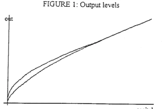
The function f(k, hIT,p) is decreasing in the tariffrate. Tariffs reduce output for two reasons, both completely standard within the Hecksher-Ohlin model of international trade. First, they distort the prices used in the decision of how to allocated the factors K and L between the intermediate goods production; for example, a labor-abundant country (meaning one that has lower K j L than the large price-setting economy) would, in the presence of the tariff, reallocate factors from the production of A to the production of B, as the tariff makes the capital-intensive good more expensive. This reallocation reduces the value of national product at international prices. In other words, for high T, the maximand of qA

+

B (which is what is maximized

by local firms) is very different from the maximand of pA

+

B (which is what determines the international purchasing power of the national output).

The second reason why T reduces productivity in this model is that it

distorts the way in which the revenue from intermediate good production is spent. In the same example, a tariff would push final goods producers to an input mix that has a higher ajb. A high tariff distorts q away from the

real opportunity cost of one intermediate good in terms of the other (which is equal to their international relative prices), leading to a solution that is suboptimal.

The losses from imposing a tariff are, of course, increasing on the tariff rate, up to a prohibitive tariff at which trade disappears.. As a proportion of total output these losses are, also. increasing on the difference between k

•

•

ratio is from the balanced growth path. the higher the proportional sacrifice from giving up the gains from trade.

Consider the difference in output between a country that has a capital-labor ratio k. and a country that has the steady-state k*. The gains from trade. as a fraction of that difference. is not decreasing in k. This is because

for a very poor economy, with very low k, the gains from trade are a very large fraction of its own output, that output is very small compared to the difference with the steady state output. As the third panel in figure 1 illus-trates, it is for middle income countries that the gains from trade are a largest fraction of the steady state output: consequently, it will be for middle-income countries that tariffs will explain a highest fraction of the total productivity residual.

3.3 The Results

We perform a levels-accounting analysis analogous to those in Hall-Jones (1997) and Klenow-Rodriguez (1996), using a variety of different data, and using the production function

F

derived from this model. The objective is to account for the differences in income between the United States and each of the countries in our sample, attributing the portions that correspond to differences in human capital. differences in physical capitaL differences in productivity emerging from tariffs, and differences from productivity emerg-ing from other unaccounted sources. Each exerci se is performed for three baseline values for the parameter Qa.

The results are summarized in the tables below-S.

Qa = 0.45 h k T a

Average 24.0% 32.9% 3.1o/c 39.9% Median 19.6% 34.3% 3.3% 41.5%

Maximum 5.6%

Top-10% 4.5%

Top -25% 3.8%

.'

•

na = 0.35 h k 7" a

Average 24.1% 27.9% 4.6% 43.4% Median 20.0% 28.6% 3.1% 43.7%

TvIaximum 12.4%

Top-10% 10.0%

Top -25% 8.5%

. As ･ｸｰ･｣ｴ･､ｾ＠ we find that the exerci se attributes about 50-60% of the cross-country variation in income to ｩｮｰｵｴｳｾ＠ and the rest to ::productivity."

More importantly. we focus now on the role of trade policy. We find ｴｨ｡ｴｾ＠ again as predicted. the 100ver (la the higher the relative importance of

tar-iffs in explaining cross-country income variations. This occurs because. the more different the capital shares in the two intermediate good sectors. the bigger the gains from trade to be realized. and hence the costlier that trade restrictions will be.

For the baseline value of na

=

0.35. we find across ali four data sets ｴｨ｡ｴｾ＠ on average, only about 5% of the total income variation can be explained by productivity differences induced by trade policy. This is only between 1/9 and 1/6 of the importance of ｯｴｨ･ｲｾ＠ unspecified productivity differences. On the other hand, the results do not seem to indicate that tariffs are unimpor-tanto In fact, for those countries that do have excessively restrictive trade policies, our t% columns show much larger numbers. In a quarter of the countries we find that between 10 and 12% of output differences can be at-tributed to tariffs (this is about 2/5 of overall productivity differences): in some countries as much as 17%. These numbers can be made much larger with lower values for the parameter Üa'

The effects of tariffs are indeed larger in some middle income countries. In generaL we find that the effect of trade policy is largest in Latin Amer-ica (BraziL ａｲｧ･ｮｴｩｮ｡ｾ＠ ｍ･ｸｩ｣ｯｾ＠ U ruguay ) ｾ＠ South Asia Ｈｉｮ､ｩ｡ｾ＠ Pakistan, Sri Lanka) and North Africa Ｈｔｵｮｩｳｩ｡ｾ＠ Algeria). In the countries mentioned, be-tween 16 to 28% of the total productivity residual can be attributed to trade policy. We find much smaller numbers for Sub-Saharan Africa, as the model predicts they are too poor. More importantly, for about half of the countries in the sample (Europe, East Asia, and most of the smaller nations) the trade policy is very similar to that of the USo and thus little of the variation can be attributed to this source. This is consistent with an explanatory variable that yields high t-statistics but low R2

4

Differences in Growth Rates

4.1

The data

Differences across countries in growth rates are also very large. For example, between 1960 and 1985, the per-capita annual GDP growth of the eight fastest-growing countries was at least 3.5% faster. per year. than that of the USo As that rate. their income as a share of US income is multiplied by between 2.5 and 3.3 in only one generation. This group included both rich and poor countries. During the same time. output per-capita grew by at least 2.5% per year less than in the US in another eight countries (all of

which happen to be African). The differences in growth rates are manifested both in terms of productivity and in terms of inputs. Even excluding African countries, there are plenty of nations that are not catching up with the USo

The relationship between trade and growth is also very pronounced. In terms of the growth rate of output, the following table summarizes the results from regressing the growth rate of GDP per-capita on various measure of trade policy.

Independent variable Coefficient t-statistic R2 Sample size SH-implicit tariffs -1.36 -3.65 0.12 98

OPEN residual 1.56 5.02 0.21 98

.6. in OPEN residual 0.96 3.05 0.09 98

SW tariffs -0.69 -1.96 0.05 73

As can be observed from the table. all the coefficients are high. have the expected signo and are significant. In terms of productivity growth similar results are obtained too.

..

"

4.2

What the model

says

There are two ways of interpreting the relationship between trade and growth in our model; in our quantitative experiments. both are going to end up being of roughly equal importance. First. and most simply. economies that reduce trade barriers have a productivity increase. for the reasons detailed in the section on leveIs. This means that the changes in trade policy can help

explain growth. Second. because the implicit technology in the model is in part determined by trade policy. we find that tariffs can affect average and marginal ｯｵｴｰｵｴｾ＠ and consequently affect the rate of accumuIation of inputs. This means that levels in trade policy can heIp explain growth.

ｃｯｭｰ｡ｲ･ｾ＠ for ｩｮｳｴ｡ｮ｣･ｾ＠ the production function for an economy without tariffs, versus the one for an economy with prohibitive tariffs (see figure 1). We know that both functions have the same leveI of output at two input leveIs: ｺ･ｲｯｾ＠ and the steady state. Since the open economy has a higher output everywhere ･ｬｳ･ｾ＠ we know that its production function is steeper for low leveIs of inputs but becomes fiatter as the economy approaches the steady state.

For very poor ･｣ｯｮｯｭｩ･ｳｾ＠ both the average and the marginal productiv-ity of inputs are higher in an open than in a closed economy. ｉｮｴｵｩｴｩｶ･ｬｹｾ＠

this means that both through an income and a substitution effect we are to observe higher savings rates in the open economy. That means that poor economies. when ｯｰ･ｮｾ＠ grow faster in ｩｮｰｵｴｳｾ＠ and this effect goes in addition to the difference in productivity.

As the economy approaches steady ｳｴ｡ｴ･ｾ＠ on the other ｨ｡ｮ､ｾ＠ we know that average productivity is still higher for the open ･｣ｯｮｯｭｹｾ＠ but marginal productivity must be lower (this has to be the ｣｡ｳ･ｾ＠ as the two economies have the same leveI of output in steady state). Now, a substitution effect goes in the opposite direction, and as we approach steady state we see that the closed economy grows faster. For economies that are not too poor ｾ＠ the gains from trade are channelled into consumption rather than investment.

are manifested in consumption much more than in output. For example. an economy with 20% of the steady state capital levei produces 5% more if it is open than if it is closed, but consumes roughly 12% more.

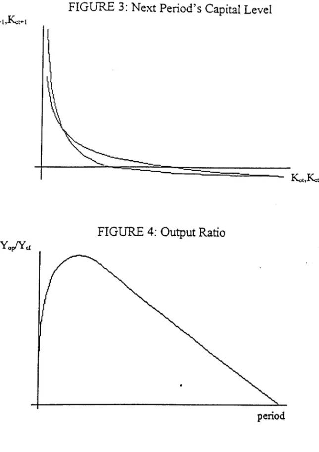
Figure 3 shows next period's capital for an open (the initially steeper curve) and a closed economy, again as functions of this period's capital. As can be seen. if the eco no mies are very poor then the savings when open can be much higher than when closed: around k = 0, the growth rate of capital is four percentage points higher for the open economy. However. as the closed economy overtakes the open economy in marginal productivity, the differences in savings leveIs begin to disappear. For an economy that has 20% of the steady state capital stock trade does not affect the accumulation of capital (all the gains from trade are consumed), and for a wealthier economy trade can actually slow down input growth (by as much as one percentage point). We obtained our results for the same baseline values for the parameter

Da used in Section 3, and the effects are robusto

Finally, figure 4 shows the ratio of output for an open over a closed econ-omy, this time along a typical transition path. \Ve start both economies with the same leveI of initial k, but have one economy open up in the first period, while the other one remains closed throughout. On impact, output in the first one becomes 11 % higher in the open economy, due to the productivity increase. Furthermore, the difference between the two keeps getting wider for a few periods. as the open economy also saves more and accumulates more capital. As both get wealthier (so the gains from trade lose importance, as they are resembling more their wealthy trading partner) and marginal productivity in the open economy gets loweL we see the closed economy be-ginning to catch up. After many periods, they indeed have similar output leveIs.

•

so paths that require more human capital accumulation display much more transitional growth for the open economy.

4.3

The results

In this section. we present two types of results. First. to evaluate the effect of trade policy variations on productivity grmvth. we do a grO\vth accounting exercise analogous to the leveIs accounting analysis performed in Section 3. Second, to evaluate the effect of trade policy levels on input growth, we

simulate several transition paths for the econornies in our data sample, under alternative scenarios for trade policy.

In table 6 (see appendix) we present an example of the results of growth accounting using changes in trade policy, for the period 1970-85.6 _{vVe only} report those countries for which the trade-policy component is most signifi-canto

For seven countries, we find that increased protectionism reduced growth relative to the US significantly (by as much as 12% in some cases). For a larger group of countries, opening up to trade contributed significantly to growth; for the top four countries (Indonesia. Tanzania, Korea and Taiwan) the contribution is between 7 and 12% of total growth relative to the US.7

For Indonesia, Korea, Ireland and Chile. for example, trade liberalization contributes more to growth than human capital accumulation. Sadly, we cannot report at this time. due to lack of data, analogous results for the period 1960-1985. Presumably, as this is the period were most Latin American and African countries de-liberalize trade, as well as when South East Asia does most of its trade liberalízation, we would see much more promínent results for that other time período

As important as the contributions to productivity are the contributions of trade to input accumulation. To assess them, we conducted the following experimento We take the capital stock of each country in our sample for 1970, 6We use the price distortion index as our variable for tariffs, and Barro-Lee for human capital. For none of our other series had we found 1970 data to run the comparison.

We used here D:a = 0.45. With lower values for this parameter, as before. the effects can get quite big. We should note that the results were fairly sensitive qualitatively to changes in D:a ; some countries that do not makc it to Table 5 have fairly strong cffects of changes in trade polic)', according to the other cxercises.

ＮＭＭＭｾＭ

-

.-relative to the USo and assign the same proportion of steady-state capital for a hypothetical counterpart in our modelo Then. for each country. we generate three paths: one for a perpetually closed economy. one for an economy that runs for four years in autarchy and then liberalizes trade. and one for an economy that opens permanently in year one. \Ve compare. at year 8. how much gwwth has been accumulated in each of the economies that liberalized ｴｲ｡､･ｾ＠ relative to the closed economy.

The following tables summarize the results for the case Cl:_a = O 35 .

For Cl:_a

=

0.35 Yap4/Ycl ｙ｡ｰｏＯｽｾｬ＠ Cop..j/Ccl CopO/Ccl J(op4/ J(cl J(opO/ J(cl

Average 1.13 1.12 1.30 1.30 1.03 1.05

Max 1.42 1.49 1.67 1.79 1.24 1.44

Min 0.98 0.94 0.99 1 0.93 0.86

1-quartile 1.02 1.00 1.19 1.14 0.96 0.94

2-quartile 1.12 1.10 1.30 1.29 1 1.01

3-quartile 1.23 1.24 1.43 1.46 1.08 1.15

st dev 0.13 0.16 0.18 0.22 0.08 0.16

As can be seen from the ｴ｡｢ｬ･ｳｾ＠ whüe for some countnes the open path leads to less growth in inputs (and even to less output 8 years down the road). for most countries that is not the case. Under the more conservative value of Cl:_a

=

OA5, we find that over 80% of the eco no mies are wealthier

if they have ｯｰ･ｮ･､ｾ＠ and practically all are consuming more along an open growth path.

5

Differences in Trend

5.1

The data

11

in our list have seen the lead expanded slightly. and the whole list has fallen behind considerably.

The fact that so many countries. most ofthem fairly ｰｯｯｲｾ＠ seem to behave as if they were on a lower-Ievel balanced-growth path. have led researchers to seek for ';development ｴｲ｡ｰｳＺｾ＠ that is. for other steady states to which poorer

economies would be converging. One problem with this notion is that these traps seem not to be infallible: many countries have avoided the ｴｲ｡ｰｾ＠ started out much poorer and yet ended up much wealthier than those that have fallen in the trapo A "selective" trap: that would only catch those countries that display a particular feature or enforce a particular policy, would be a more appropriate concept given the evidence.

Can bad trade policy be such selective trap? Before we consider the model, notice the second part of Table 6. Trade barriers for this group of countries are significantly higher than for the world as a whole. For ･ｸ｡ｭｰｬ･ｾ＠

the Swagel-Wagner tariffs: which are 18% in the average country: are 30% in the average country for our "development trap list." The incidence of non-tariff restrictions, according to Sachs-Warner, is twice as much among the list than in the whole sample. The mean OPEN residuaL by construction equal to zero for the whole world. averages -0.30 (a whole standard deviation) for these countries.

5.2 What the Model Says

The model we consider in this paper has such selective development traps. We have seen that, for tariffs that are either O or x, there is a unique, globally

stable steady state. That is also the case for tariffs that are positive but low. However, as it turns out, given other parameters there is a positive ｴ｡ｲｩｦｦｬ･ｶ･ｬｾ＠

call in 7, such that if T

>

7 there is a second steady state, lower than k* (and

decreasing in T). The reason is that, for positive T, the map y(k) is no longer concave, as there is a leveI of k at which its first derivative jumps up (that is the leveI of k at which the economy switches from trade to autarchy; that is, where K:(T) = k). For a large enough T, the discontinuity is large enough that it makes the steady-state Euler equation have two solutions: there are two steady states (the one shared with the large price-setting economy. and another one strictly lower). 8

BThe higher T, also, the Iower the k at which the discontinuity occurs. That is why for

•

5.3

The Results

We have calculated the value of 7. the tariff leveI at which the development traps occur. for alternative values of Da· Those are presented in the following table'

Da T kjk* j(k)j j(k*) 0.45 0.202 0.159 0.294 0.40 0.461 0.150 0.282 0.35 0.832 0.133 0.260 0.30 1.465 0.105 0.222 0.25 3.265 0.056 0.146

Unlike the high steady state, the lower steady state Te is decreasing in T. Figure 3 presents the values of k and output at the lower steady state, as a function of tariffs, as they increase beyond 7

6

Conclusion

References

[1] Barro,R. and J. W. Lee(1996) "International Measures of Schooling Years and Schooling Quality, " American Economic Review, 86, 2, pp. 218-223.

[2] Chari,

V.,

Kehoe, P. and E. McGrattan(1996) The Poverty of Nations:

A

Quantitative Exploration, FRB of Minneapolis Research Department Staff Report 20.

[3] Edwards,S.(1993) "Openness, Trade Liberalization and Growth in Devel-oping Countries," Journal of Economic Literature, 31, 3. pp. 1358-1393.

[4]

Hall,R. and C. Jones(1996) "The Productivity of Nations, " NBER work-ing paper 5549.

[5] ｌｵ｣｡ｳｾ＠ R. and E. Prescott(1971) "Investment Under Uncertainty/' Econo-ｭ･ｴｲｩ｣｡ｾ＠ 39, 5. pp. 659-682.

•

[6] Mankiw. G., Romer. D. and D. Weil(1992) "A Contribution to the Em-pirics of Economic Growth." Quarterly Journal of Economics. 107. 2, pp. 407-437.

[7] Parente. S. and E.C. Prescott(1994). Barriers to Technology Adoption and Developmentl Journal of Political EconomYl v.102(2): 298-321. [8] Rebelo, S. (1991) "Long Run Analysis and Long-Growth:" Journal of

Political ｅ｣ｯｮｯｭｹｾ＠ ＹＹｾ＠ 3, pp. 500-521

..

'

TABLE 6

Contribution to growth in productivity from changes in trade policy and in inputs

(1970-1985, a.

=

0.45)

gY gH gK _{delta t gA.}

TOGO -0.272 0.446 0.153 _{-0.116 -0.761}

KENYA -0.056 0.236 -0.102 _{-0.095 -0.095}

JORDA.l'i 0.630 0.273 0.376 _{-0.039 0.115}

URUGUAY -0.296 0.049 0.073 _{-0.057 -0.361}

GUYANA -0.662 0.034 -0.175 _{-0.055 -0.466}

" CYPRUS 0.302 0.033 0.035 -0.036 _0.221

"

GREECE 0.163 0.036 0.113 _{-0.025 0.033}

l\Lo\LA YSIA 0.462 0.102 0.249 0.007 _0.104

CANADA 0.229 0.014 0.072 0.007 _0.135

FRANCE 0.033 0.055 0.050 0.003 _-0.030

JAP.I1,.N 0.212 0.023 0.136 0.010 -0.007

ICELA.'ID 0.363 0.021 0.091 0.013 _0.242

BELGI'lRv1 0.045 0.007 0.017 0.014 _0.007

CHILE -0.330 0.010 -0.089 0.023 _-0.279

IRELAND 0.127 0.013 0.124 0.034 _-0.049

PAJ,\íAMA 0.049 0.057 0.027 0.050 _-0.085

IRAN -0.050 0.279 0.075 0.055 _-0.453

TAlWAJ,'i 0.671 0.106 0.272 0.071 _0.222

KOREA 0.691 0.064 0.343 0.083 _0.196

T AJ,\lZANIA -0.159 -0.023 -0.036 0.097 -0.196

INDONESIA 0.717 0.114 0.433 0.124 0.046

FIGURE 1: Output

leveIs

l(k)

•

capital

FIGURE 2: Consumption Ratio

capital

I .

I "

•

FIGURE 3: Next Period's Capital LeveI

•

FIGURE 4: Output Ratio

period

N.Cham. P/EPGE _{SPE F383b} Autor: Ferreira, Pedro Cavalcanti.

Título: Barriers .to trade : baqiers to growth.

1111111111111111111111111111111111111111

ｾｾｯｾｾ＠

14 I ' ""

FGV - BMHS , N" Pat.:FI54/98

: "'li': ｾ＠

000086214

•

•

_,.

...