Improving mutual fund market timing measures: a markov switching approach

FUNDAÇÃO GET ÚLIO VARGAS —

FGV

ESCOLA DE PÓS-GRADUAÇÃO EM ECONOMIA —

EPGE

CURSO DE MEST RADO EM ECONOMIA

IMPROVING MUT UAL FUND MARK ET T IMING

IMPROVING MUT UAL FUND MARK ET T IMING

IMPROVING MUT UAL FUND MARK ET T IMING

IMPROVING MUT UAL FUND MARK ET T IMING

MEASURES: A MARK OV SWIT CHING APPROACH

MEASURES: A MARK OV SWIT CHING APPROACH

MEASURES: A MARK OV SWIT CHING APPROACH

MEASURES: A MARK OV SWIT CHING APPROACH

Dissert ação submet ida à

Congregação da Escola de

Pós-Graduação em

Economia (EPGE) para

obt enção do grau de

Mest re em Economia

Aut or: Rogério Mazali

Orient ador: Marco Ant ônio César Bonomo

Rio de Janeiro

Julho 2001

IMPROVING MUT UAL FUND MARK ET T IMING

IMPROVING MUT UAL FUND MARK ET T IMING

IMPROVING MUT UAL FUND MARK ET T IMING

IMPROVING MUT UAL FUND MARK ET T IMING

MEASURES: A MARK OV SWIT CHING APPROACH

MEASURES: A MARK OV SWIT CHING APPROACH

MEASURES: A MARK OV SWIT CHING APPROACH

MEASURES: A MARK OV SWIT CHING APPROACH

Rogério Mazali

Rio de Janeiro

Julho 2001

A boa educação é a moeda de ouro: em toda parte tem valor.

(Pe. Antônio Vieira)

Acknowledgement s

Acknowledgement s

Acknowledgement s

Acknowledgement s

I’d like t o t hank, first of all, my parent s, t he great est

support ers of t his work, who had pat ience t o st and my

idiosyncrasies along all t hese years. I’d like t o t hank my

advisor, prof. Marco Ant onio Bonomo, for t he ideas used t o

complet e t his work and Drs. Ricardo Simonsen and Gyorgy

Varga, for helpful comment s. I’d like also t o t hank Dr.

Ricardo Simonsen, for kindly allowing me t o use his dat a base.

Last of all, I’d like t o t hank professors Jack Schecht man,

Ricardo Cavalcant i, Marco Bonomo, René Garcia, Aloísio

Araújo, Fernando de Holanda Barbosa and Maria Crist ina

T erra for helping me wit h my next st ep.

IMPROVING MUTUAL FUND MARKET

TIMING MEASURES: A MARKOV

SWITCHING APPROACH

1

Rogério Mazali

Advisor: Marco Antonio César Bonomo

Fundação Getúlio Vargas. Rio de Janeiro, Brazil

August 3, 2001

Abstract

Contents

1 Introduction 2

2 Popular Measures of Market Timing 3

2.1 The Dummy Variable Model . . . 3

2.2 The Squared Regressors Model . . . 4

3 The Markov Switching Timing Model 5 3.1 Measuring timing performance . . . 6

4 Tests of Hypotheses 8 4.1 Testing for existence of market timing strategies . . . 9

4.2 Testing for efficiency of market timing strategies . . . 10

5 Results 11 5.1 Methodology . . . 11

5.2 Data . . . 11

5.3 Simulation results . . . 12

5.3.1 Simulation 1: managers fail as much as succeed in pre-dicting the state of nature . . . 12

5.3.2 Simulation 2: a successful manager . . . 13

5.3.3 Simulation 3: timing at points other than zero . . . 15

5.3.4 Simulation 4: successful but conservative manager . . . . 17

5.3.5 Simulation 5: Continuous market timing . . . 19

5.3.6 Simulation 6: successful market timing with some errors . 21 5.4 Estimation Results . . . 22

5.4.1 Fixed probabilities model estimates . . . 22

5.4.2 Changing probabilities model estimates . . . 23

5.4.3 Comparison between models’ estimates . . . 25

1

Introduction

Investors always seek for ways to evaluate investment performances in a way so that they can assure themselves they are making the best choice. Among the characteristics investors usually evaluate are expected return, total risk, asymmetry, systematic risk and, in the case of active mutual funds, manager’s ability in selecting assets and manager’s ability to respond to market movements by choosing (less) riskier portfolios when market portfolio is expected to be bullish (bearish). The former of these characteristics is commonly referred as ”selectivity”, while the last is usually called ”market timing”.

In the Sharpe (1964) version of CAPM, an efficient portfolio is usually a linear combination of the risk free asset (if it exists) and the market portfo-lio, if the risk free rate is below the expected return of the minimum variance portfolio. Managing portfolios actively, one can achieve higher returns than it could be achieved handling a passive strategy portfolio of just carrying aÞxed combination of market portfolio and the risk free asset. So, if an investor is seeking for an unconditionally dynamically efficient investment, in the case of mutual funds, knowing whether a fund is managed actively and how changes in expectation of future returns of assets affect fund’s risk proÞle would be useful information.

Obtaining information about portfolios consulting directly all fund adminis-trators could be, however, very costly to most investors. Beside that, as pointed by Lakonishok et al. (1992), funds may be subject to ”window dressing” by managers because of agency costs between them and investors. So, a frame-work in which it could be inferred would be a relatively cheaper alternative that could serve to this purpose. Henriksson and Merton (1981) suggest that market timing could be measured by making a slight modiÞcation in the CAPM framework. Their approach is equivalent to introducing a dummy variable in the beta coefficient, which allows for the beta coefficients to be different when market portfolio excess returns are positive (bull market) and negative (bear market). Another approach, due to Treynor and Mazuy (1966), is to estimate a parabolic curve and test for its convexity.

Despite these simple models can work quite well in evaluating past market timing performances, they can underestimate differences between beta coeffi-cients, because managers choose portfolio allocation based on their predictions of asset returns that often fail. By using realizedinstead of expected returns to split the sample, these traditional models attribute high beta when beta is low and low beta when beta is high to every observation in which managers’ expectancy fails.

We propose an alternative framework for estimating betas in the presence of market timing in which the possibility of manager’s expectancy failure is taken into account. We also allow managers’ expectancy of market returns to be autoregressive in a way similar to that used by Hamilton (1989). He created what he called the Markov Switching model of changes in regime to explain

the next section, we describe in detail the most popular models in Þnancial literature used to evaluate market timing. In section 3, our basic model and some extensions are developed. Section 4 will discuss theoretical issues related to hypothesis testing using the framework developed in section 3. In section 5, we show results of estimations of our models using simulated and Brazilian stock mutual funds data. We use simulated data to ilustrate the ideas explained when we develop our basic model. For real world data, we compare the results obtained with the models we developed to those obtained used the models de-scribed in section 2. In the last section we display our conclusions and questions for further research.

2

Popular Measures of Market Timing

Before we develop our market timing models, we will brießy expose the most popular models used to estimate market timing and rank funds according to these estimates: the dummy model and squared regressors model (or quadratic regression). In both models, the central idea is the same: if a manager is able to anticipate future returns, she will change her exposition to systematic risk in order to capture a higher risk premium when market is bullish and reduce losses when market is bearish. If she is successful in doing that, it will result that, if we plot excess returns of fund and market portfolio returns on a scatter diagram, the points will seem to cluster around a convex curve. The two models cited above were developed to capture this effect. We will begin describing the dummy variable model, describing then the quadratic model. The following discussion is based on Sharpe, Alexander and Bailey (1991).

2.1

The Dummy Variable Model

The dummy variable regression is the approach to market timing where the sample is ”split” in two: the ”bull market” and the ”bear market” subsamples. It then estimates two beta coefficients, one for each subsample. A successful market timer will anticipate market returns and select the high beta portfolio when market is bullish and the low one when market is bearish. In other words, the CAPM line slope will be greater for the bull market subsample than it will be for the bear market subsample. This model was Þrst proposed by Merton (1981) and Henriksson and Merton (1981). Despite these articles did not state the equations in terms of Dummy Variables, it is easy to show that their notation is equivalent to the model stated in Sharpe, Alexander and Bailey (1991).

Such a relationship can be estimated by altering the Sharpe version of the CAPM equation a little. Denoting the return of fund i by Ri, the return of the market portfolio by Rm and the return of the risk free asset by Rf, ex-pected returns of mutual fund i share and the market portfolio are related in the following way:

E[Ri−Rf] = βiE[Rm−Rf] (1)

The empirical version of the CAPM can be written as:

where²tis a disturbance term. We now introduce a constant term, as in Jensen (1968), and the dummy variable, deÞned the following way:

Dt=

½

1, ifRmt−Rf t≥0

0, ifRmt−Rf t<0

The dummy variable separates bull and bear market subsamples. The altered CAPM equation will be then:

[Rit−Rf t] = α+ βi1[Rmt−Rf t] + βi2.Dt.[Rmt−Rf t] + ²t (3)

Theβ_2icoefficient represents the increase in risk exposure (increase in beta) that the manager adopts when the market is bullish. As this equation has only linear relations between the dependent variable and the coefficient, OLS estimates can be used. Our measure of market timing will be the value of parameterβ_i2. To test for the efficiency of market timing strategies, our null hypothesis will be

H0 :βi2 = 0. With OLS estimates, the Student-t distribution can be used to

obtain critical values of the test.

If someone wants the coefficients to represent values of beta of bull and bear markets, the equation to be estimated will be:

[Rit−Rf t] = βi1.D1t.[Rmt−Rf t] + βi2.D2t.[Rmt−Rf t] + ²t (4)

where D1t =

½

1, ifRmt−Rf t≥0

0, ifRmt−Rf t<0 and D2t =

½

1, ifRmt−Rf t<0

0, ifRmt−Rf t≥0 . To test for the efficiency of market timing strategies, our null hypothesis is now

H0 :βi1 = βi2. and can be carried out with Student-t distribution to obtain

critical values of the test. Market timing here is measured as the difference between the highest and the lowest beta. All along this text, it will be convenient for us to adopt the equation deÞned by equation 4 when talking about Dummy Timing Models. On the appendix, however, we show estimates using the simpler equation 3.

2.2

The Squared Regressors Model

One implicit assumption of the Dummy timing model is that there are only two betas and the manager changes between them. But a manager may respond differently in terms of changing betas to different values of market portfolio returns. In this sense, the greater is this return, the greater may be the beta of a successful market timer. To capture this effect, a quadratic regression on the excess returns of market portfolio may be much more convenient than the one shown above. On this approach, due to due to Treynor and Mazuy (1966), the researcher willÞt the data on a parabola rather than on lines, as the other approach. The equation to be estimated is then:

[Rit−Rf t] = α+ βi1[Rmt−Rf t] + βi2[Rmt−Rf t]2+ ²t (5)

where²tis a disturbance term. Again, as in the Dummy Model, the equation to be estimated is linear in relation to parameters. OLS can then be used to esti-mate coefficients and Student-ttests can be applied to test for their signiÞcance. The measure of market timing in this model will be the value of parameterβ_i2.

this parameter will be an indication that market timing strategies applied by the manager are successful. A negative one will mean failure on these strategies and a non-signiÞcant one will indicate median performance.

3

The Markov Switching Timing Model

In this section, we develop a simple framework for estimating betas in the pres-ence of market timing using the non-observable fund manager’s expectancy of market portfolio as a state variable. As in Treynor and Mazuy (1966), Mer-ton (1981) and Henriksson and MerMer-ton (1981), our departure is the well known Sharpe empirical version of the CAPM framework described by equation 1.

We now introduce time structure in this model. Let St denote the regime variable, which, for us, will be the manager’s expectancy of future market be-havior. If he is optimistic and expects that market portfolio return would be low, then St = 1, and if he is optimistic, St= 2. When the manager is opti-mistic, he handles a portfolio with a high beta, in order to receive the premium for bearing higher risk. When he is pessimistic, he handles a conservative port-folio in order to avoid high losses. This regime variable is supposed to follow a Þrst order Markov chain with a matrix of transition probabilities P2×2. In

principle, we do not make any restrictions in the transition probabilityP. With this structure, equation 1 turns out to be:

E[Rit−Rf t] = βiStE[Rmt−Rf t] (6)

where St = 1,2 . We assume also that the error in prediction of fund excess returns has a normal centralized distribution, so that:

[Rit−Rf t] = βiSt[Rmt−Rf t] + ²t (7)

where²t∼N(0,σ2).

Formally, we can include the state variable in the equation. For this

rep-resentation, deÞne variables ξ_1t= ½

1, ifSt= 1

0, ifSt= 2 , ξ_2t =

½

0, ifSt= 1

1, ifSt= 2 and ξ_t= £ξ1t ξ2t

¤0

. So, equation 7 becomes:

[Rit−Rf t] = hβi,ξti[Rmt−Rf t] + ²t (8)

whereβi=

£

β_i1 β_i2 ¤, and

ξ_t= P.ξ_t−1+ vt (9)

where vt ≡ ξt−E(ξt|ξt−1,ξt−2,ξt−3, ...)1. So, we have the equations to be

estimated, which are deÞned by equations 8 and 9. For the theoretical framework to be complete, the remaining step is to discuss about the statistical properties of the hypotheses test, what will be the subject of the next section.

1_{If a processξ}

t has the Markov Property, then we haveE(ξt|ξt−1,ξt−2,ξt−3, ...) = P.ξt.

DeÞningvt ≡ξt−E(ξt|ξt−1,ξt−2,ξt−3, ...), equation 9 follows immediately. For details, see

3.1

Measuring timing performance

The model we have just described provides a way to unbiasedly estimate betas of a mutual fund that has its portfolio managed actively through market timing strategies. It also allows an investor to test for the hypothesis that such strate-gies are adopted by the fund manager, as will be seen in a later section. But investors may want not only to estimate betas and carry out test hypotheses correctly. They may want to compare fund performances and rank mutual funds according to how well each fund manager has done in market timing strategies. For that purpose, the model just developed has little information to aggregate. Despite that, as will be shown in this section, a little modiÞcation in this model can be done in order to adapt it to give the investor some information about timing performance. This will be done by replacing our model in the context of Markov Switching with changing transition probabilities, a model developed by Diebold et al (1996).

This approach to Markov Switching processes changes from Hamilton’s in an important point: transition probabilities may change over time. These vari-ations may be due to changes in variables that are important to deÞne the regime that will be revealed as the actual one. For example, a meteorologist may have two states of nature, let’s say sunny and rainy weather, for which she may have to make probability predictions daily. Applying Hamilton’s model, the meteorologist may then to obtain transition probabilities estimates that will enable her to tell what is the probability of raining today given just the weather yesterday. But the probability of raining may not depend just on the weather yesterday, it may depend on variables such as air humidity and wind speed. If we state transition probabilities as functions of these variables, we may aggregate important information that can improve substantially our predictions about the probability of raining each day.

In our model, managers’ decisions about what position to take (high or low beta) are conditioned to their expectancy about future returns of the market portfolio. If they are well succeeded in their strategies of market timing, they will adopt high beta positions when the return of the market portfolio is high and low beta positions when this variable has a low value. Therefore, if we state transition probabilities as functions of market portfolio returns, what we will observe is that probabilities of adopting riskier positions will be strongly and positively related to market portfolio returns and probabilities of adopting low risk positions will have strong negative relations to market portfolio returns. On the other hand, the reverse relations will be found for funds managed by people that systematically have mistaken predictions about future market portfolio returns.2

What we do to capture this effect is, following Diebold (1996), to state transition probabilities in logit equations, so that the relations just described can be captured. Our model becomes, then:

[Rit−Rf t] = βiSt[Rmt−Rf t] + ²t (10)

where²t∼N(0,σ2).

2_{As time tportfolio is formed at time t}

Formally, we can include the state variable in the equation. For this

rep-resentation, deÞne variables ξ_1t= ½

1, ifSt= 1

0, ifSt= 2 , ξ2t =

½

0, ifSt= 1

1, ifSt= 2 and ξt=

£

ξ_1t ξ_2t ¤0. So, equation 10 becomes:

[Rit−Rf t] = hβi,ξti[Rmt−Rf t] + ²t (11)

whereβ_i= £ β_i1 βi2

¤0

, and

ξ_t= Pt.ξt−1+ vt (12)

where vt= ξt−E(ξt|ξt−1,ξt−2,ξt−3, ...)3. Note that the transition probability

matrix may now change over time, and it will do it following the logit equations stated below:

Pt=

·

p11

t p21t

p12

t p22t

¸ =

"

ex p(xt.θ1)

1+ ex p(xt.θ1) 1−

ex p(xt.θ2)

1+ ex p(xt.θ2)

1− ex p(xt.θ1)

1+ ex p(xt.θ1)

ex p(xt.θ2)

1+ ex p(xt.θ2)

#

(13)

wherext=

¡

1 Rmt

¢

1x2is the probability explaining variables andθi, i= 1,2

are 2x1 parameter vectors. Once we have estimated the parameters of the model, we can then create a measure of performance based on these estimations. Before we proceed on doing that, it is worth to spend some time discussing the interpretations the parametersθi might have.

Note that the elements of the principal diagonal ofPtrepresent the proba-bilities of staying in the current position, while the other elements of the matrix represent the probabilities of changing to the other position. It is easy to see that the equations forpii

t can be restated as:

ln µ

pii_t

1−pii t

¶

= xt.θi (14)

Then we have that:

θi= d

dxt

ln µ

piit

1−pii t

¶ = d

dxt

lnpii_t − d

dxt

ln¡1−pii_t¢ (15)

Equation 15 tells us that the parameter vectorsθi, i= 1,2are the difference of the gradients of the logarithms of the probability of staying in the current position and of the probability of changing it. In other words, the second coordi-nates ofθi=

¡

θ0_i θ1_i ¢represent the difference between percentual change an inÞnitesimal variation on the market returns causes on the probability of staying in the current position and the percentual change it causes on its complement. This interpretation of θi makes θ1i, i = 1,2 natural candidates for measures of market timing, except for the fact that variations on probability values are percentual (because of the logs). If we accept these coefficients as measures of market timing, we will rank a fund that, on the presence of an augment on the market returns, changes its probability of adopting the riskier position from 0.0001 to 0.01 (a 9999% change) as a better fund than another that, on the same

3_{If a processξ}

t has the Markov Property, then we haveE(ξt|ξt−1,ξt−2,ξt−3, ...) = P.ξt.

DeÞningvt ≡ξt−E(ξt|ξt−1,ξt−2,ξt−3, ...), equation 9 follows immediately. For details, see

situation, changes this probability from 0.25% to 0.50 (a 100% change). Clearly, the change on the last fund probabilities is much more signiÞcant than the one in the former. For this reason, the coefficientsθ1_i are not such good measures of market timing performance. For that purpose, we need a measure that gives us information about absolute changes in the probability values instead of relative ones.

Recall from equation 13 that, once we have parameter estimates, the only variable still missing for us to calculate transition probabilities is the market portfolio return. As for some given value of Rmt we are able to compute the transition probabilities, we can establish some measure of high and low returns and compute the transition probabilities associated to this arbitrary values. We can than measure how these probabilities vary with changes from low to high values in the market portfolio returns as a measure of market timing perfor-mance. The ”Timing Measure” can then be stated as follows:

T M = ¡p22¡RHm

¢

−p22¡RLm

¢¢

+ ¡p12¡RHm

¢

−p12¡RLm

¢¢

(16)

or, equivalently:

T M = ¡p11¡R_mL¢−p11¡RH_m¢¢+ ¡p21¡RL_m¢−p21¡R_mH¢¢

where RH

m and RLm correspond to the high and low market portfolio returns, respectively. The chosen low (L) and high (H) values of the IBOVESPA return were RL

m = Rm−2s(Rm) and RHm = Rm+ 2s(Rm), respectively, s(Rm) for standard deviation of market portfolio returns, because two standard deviations constitute a clear departure from the mean, as approximately 95% of a normal distribution is between these two values. The ”Timing Measure” calculates how much the probability of going to or staying in the riskier position changes when market return changes from low to high values, or, from another point of view, how the probability of going to or staying in the safer position changes when market returns are reduced from high to low values.

We have then our measure of market timing performance, what enables us to compare and rank funds according to this criterion. In a later section, we apply this formula to Brazilian data and compare the results with other measures of market timing performance.

4

Tests of Hypotheses

4.1

Testing for existence of market timing strategies

To test for the presence of a market timing strategy in a mutual fund’s manage-ment, we need to test, inÞrst place, if the data permits us to say that there are really two regimes against the alternative of only one. Our null hypothesis will be thenH0 :βi1 = βi2. Unfortunately, this hypothesis cannot be tested using

the usual likelihood ratio test. One of the regularity conditions for the likeli-hood ratio test to have an asymptotic χ2 _{distribution is that the information}

matrix be nonsingular. This condition will fail if the true number of states is 1 instead of 2. Hansen (1996) proposes a simulation method to approximate the asymptotic distributions and applies it to the threshold model. Hansen (1992) proposes another approach for the speciÞc case of Markov Switching (MS) mod-els, where, in addition to the identiÞcation problem, there are identical null score matrices under the null hypothesis. According to Garcia (1998), ”the author considers the likelihood function as a function of unknown parameters and uses empirical process theory to bound the asymptotic distribution of a standardized LR statistic. For simple MS models (...), the method involves the evaluation of likelihood across a grid of different values for the mean and transition probabil-ity parameters, the parameters of interest of in this model. For each set of such values, the constrained likelihood function need to be optimized with respect to the nuisance parameters of the model. Even for the small dimension of the space of parameters of interest in this simple model, the computational bur-den can be important if the grid search over the parameter space is extensive. therefore the use of this method for the more elaborate MS models in practice does not appear very promising. Moreover, Hansen’s method provides a bound for the LR statistic and not a critical value, which means that the tests may be conservative.” Because of these reasons just discussed, we will not follow Hansen in this paper. Garcia (1998), in his similar but alternative approach, provides approximations for the asymptotic distributions of LR statistics for the most used MS models. He avoids Hansen’s problems by treating the transition probabilities parameters as nuisance parameters and stating the null hypothesis solely in terms of parameters governed by the Markov variable (mean, variance or autoregressive coefficients). Unhappily, he does not provide tables for the MS model with switching in the coefficients. The asymptotic distribution of the LR statistic will be data dependent, so it will be impossible to derive a distribution that can be used with any database. For instance, we will be using the values Garcia provides for his model with MS in the level of variables4_.

If we do not reject the null hypothesis that there is one state of nature, weÞnd evidence that there is only one beta and the manager does not change his exposition to systematic risk with changes in his expectations about future returns. Therefore, we Þnd evidence that there is no market timing strategy on the fund’s portfolio management. On the other hand, if we reject the null hypothesis of only one beta, weÞnd evidence that there are, in fact, two different positions adopted by the manager and he switches between them. In other words, the manager adopts some market timing strategies.

4.2

Testing for e

_ffi

ciency of market timing strategies

If someone is willing to invest some money in an actively managed fund, he may want to do it in the most well managed fund. In an earlier section, we spent some time discussing how an investor willing to compare and rank funds according to their respective market timing performances. But the investor may not only want to do this. She may want to know which of these performances are signiÞcant and which funds you can say that just have lucky managers. To do that, he may want to carry out some hypotheses testing. Unfortunately, it is only possible to do that for the changing probability model, for which a measure of timing performance has been built. For this model, we can build a LR test in which we test for the statistical signiÞcance of the market returns variable on the probabilities logit equation. Our null hypothesis will be then

H0:θ11,θ12= 0. Not rejecting the null hypothesis implies that market portfolio

returns do not help explaining variations on transition probabilities.

Recall from the discussion of the timing measure we have built on the pre-ceding section that, for a successful actively managed fund, we will observe strong and positive relations between the probabilities of high beta positions and market portfolio returns and low risk position probabilities will have strong negative relations to market portfolio returns. On the other hand, the reverse relations will be found for funds managed by people that systematically have mistaken predictions about market portfolio returns. Not rejecting the null hy-pothesis then implies that none of this relations is clearly signiÞcant, and you cannot say any success is not only due to luck. Rejecting the null hypothesis implies that future returns help to explain how managers control risk of funds’ portfolios and that relations found are signiÞcant. Positive relations between high beta probabilities and future returns and negative between low beta prob-abilities and market returns together with rejection of the null hypothesis would be a clear sign of success, while the reverse relations together with rejection of

H0would be a clear sign of failure. Any other relations together with rejection

ofH0 would arise an ambiguous sign: the manager may succeed in anticipating

high returns but fail in anticipating low returns or vice-versa. To see which of the effects is most important, the investor can look at the sign of the timing measure: if it’s positive, it is a sign that successes are more important than failures, a negative one would mean failures are predominant.

As accepting the null hypothesis as the true one does not have any impli-cations to parameters except those considered null by H0, the identiÞcation

5

Results

5.1

Methodology

Since we have developed our model, we can start now discussing estimation methodology and the results found. In order to test wether our timing mod-els have the desired properties that we have brießy treated at earlier sections and will describe in detail at a further section, we will simulate some data in convenient ways so we can compare results we get in estimating timing using our models and the traditional models of market timing and applying the corre-spondent hypotheses test methodology. We then proceed to the estimation and hypotheses testing using real data described on the next subsection, and com-pare our results with the ones obtained using the models described in section 2. We divide our sample in quartiles by the several timing measures including ours. We then proceed to the construction of matrixes that relates quartiles of the funds according to our measure and one of the preexistent ones. We do the same thing dividing our sample in two (above and below the median value) and then interpret the results.

Either on the simulation or on the real data proceedings, theÞrst model we have to estimate is given by equation 7. We estimated parameters using max-imum likelihood. Since we suppose the ²t’s are normally distributed, we know the likelihood function for all states of nature. Following Hamilton (1994), we then construct smoothed probabilities in order to get a maximum likelihood function that weights states of nature according to its probability of having oc-curred given the value of observation. We then maximize the likelihood function numerically using theEM algorithm developed by Dempster, Laird and Rubin (1977) as described by Hamilton (1994). The numerical routine was constructed using MATLAB°R programming. We then proceed to hypothesis testing about the number of states of nature, listing then results found.

We then proceed to estimate the parameters for the changing probabilities model. Again, we assume normal distribution of the²t’s and estimate parame-ters by maximum likelihood using again MATLAB°R programming to execute the numerical routine. For this model, we used the Nelder and Mead (1965) Multidimensional Unconstrained Non-Linear Minimization method to minimize the symmetric of the likelihood function. We then proceed to hypothesis testing for the signiÞcance of the future market portfolio variable on the logit equations of the transition probability matrix. The results obtained are then displayed and we start calculating our ”Timing Measure” as deÞned by equation 16, displaying the results obtained.

5.2

Data

we took was the Brazilian stock index IBOVESPA closing value, for which we proceeded the same way as with fund data. The risk free proxy asset used was the CDI (Interbank Depositary CertiÞcate) weekly return taken the same way as IBOVESPA and fund data. The IBOVESPA and CDI data were taken from the Economatica°R database.

5.3

Simulation results

At this section, we will test wether our models have the desired properties that we have argued until now. We will do that by simulating convenient sets of data and estimating parameters using our models and traditional ones. We expect that, for these simulated data, traditional models and ours have quite different behaviors. These differences will be described in detail when we explain how and why we simulated data the way we did. The simulations were carried out using MATLAB°R programming, and the programs used in the simulations are in the Appendix. After that we will proceed to estimation using real world data, what will be the subject of the next subsection.

5.3.1 Simulation 1: managers fail as much as succeed in predicting the state of nature

On earlier sections, we argued that traditional measures of market timing can underestimate beta differences when managers fail as much as succeed in their predictions about future states of nature (bull or bear market). If it happens, there will be observations where fund portfolio betas are low when market return is high and vice-versa. If we plot data of this fund on a scatter diagram, what we will observe is points clustering around two lines that cross one another. Traditional ways of estimating market timing do not predict that. The dummy approach proceeds as if it split the sample in two and then estimated one beta for each part of the sample. The problem is that, in the case just described, the fund portfolio will have two betas in both parts of the sample. The OLS estimates will then give average estimates of beta for both parts of the sample, underestimating the difference between then.

Similar problems will be faced by the square factor model. This model esti-mates a parabolic function of market portfolio returns, considering a signiÞcant positive coefficient for the square of the market portfolio returns as evidence of efficient market timing performance. Facing data clustering around two lines instead of one curve, OLS estimates will tend to underestimate the square co-efficients, rejecting the presence of market timing.

Our market timing model is supposed to capture this kind of situation, giving estimates of two betas. The advantage of MS models in this case is that it does not ”split” the sample in two as does the dummy approach. Instead, it attributes probabilities (the smoothed probabilities) of one observation coming from one or another part of the sample.

used as the market portfolio, and the CDI series described on the same subsec-tion is used as riskfree asset. TheÞrst disturbance determines to which of the lines the observation will belong. A positive entry will give it to the steepest line, while a negative one correspond to an observation belonging to the other line. Finally, the other disturbance term is added. We then estimate parame-ters using the MS model and also the dummy and square ones. The simulated parameters are exposed in Table 1, as long as the estimation results:

Table 1

Model: Simulated CAPM Dummy Square MS Model

p11 0.500 - - - 0.6126

p12 0.500 - - - 0.3874

p21 0.500 - - - 0.5372

p22 0.500 - - - 0.4628

β₁ 0.500 1.7556 2.0099 1.7902 0.5476

β₂ 4.000 - 1.5271 -2.2345 3.9319

σ 0.025 0.1068 0.1057 0.10511 0.0247

loglikelihood - 85.0164 - - 182.4442

test statistic - - -1.4909 -1.86053 194.8557* test type - - Student-t Student-t LR+ * signiÞcant at 95% percent of signiÞcance

+ _{according to the distribution derived by Garcia (1998), p. 773, table 1A.}

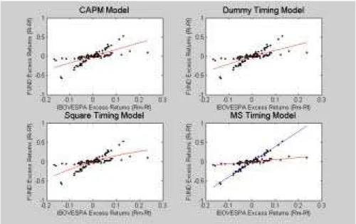
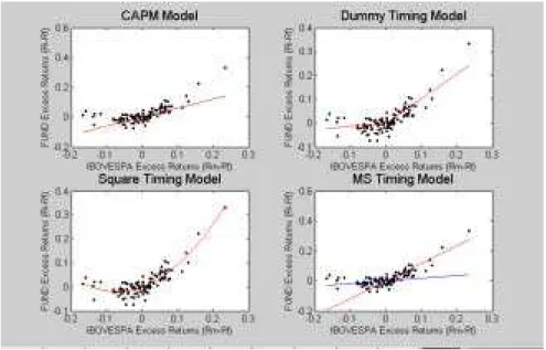
From the table above we are able to see that using Dummy and Square models we accept the null hypothesis that there is only one beta. In these models, it means that the manager do neither fully succeed nor completely fail in her attempts to predict the future, what is correct, as the data we simulated reßects the situation where she correctly anticipates states of nature in half of the situations but is mistaken on the other half. What these models do not capture is that, despite the manager is not a well succeeded market timer, she is attempting to anticipate future returns of the market portfolio. This can be veriÞed by our MS Model, as we reject the null hypothesis of only one beta. The graphics inÞgure 1 show how models’ estimatesÞt the simulated data.

We can clearly see that the clustering around two different lines affect the estimation of Dummy and Square Timing models, making their estimates similar to those obtained by simple CAPM. But the estimates obtained by the MS ModelÞts data quite well, not underestimating differences in betas as the other models do.

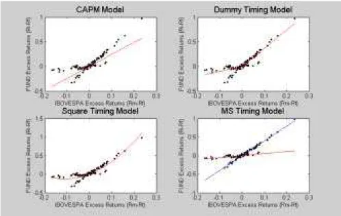
5.3.2 Simulation 2: a successful manager

Figure 1: managers fail as much as succeed

her exposition to systematic risk, meaning that fund’s beta is high, and when it is negative, she reduces it, and beta is low. The slope values are the same 0.5 and 4.0 seen on simulation 1. What is different is that all observations in which excess return on the risk free asset of the market portfolio is positive are treated as belonging to the part of the sample with the higher beta. Negative excess returns imply that the observation associated with them belong to the part of the sample with the lower beta. The results are shown in Table2:

Table 2

Model: Simul. CAPM Dummy Square MSFP MSCP

θ0₁ - - - 21.12338

θ0₂ - - - -13.778606

θ1₁ - - - -4267.9194

θ12 - - - 2979.2339

p11 - - - - 0.47483

-p12 - - - - 0.52517

-p21 - - - - 0.48404

-p22 - - - - 0.51596

-β₁ 0.500 2.2746 0.43341 2.09214 0.43518 0.43345

β₂ 4.000 - 3.93051 11.8093 3.9325 3.9305

σ 0.025 0.11438 0.023461 0.05303 0.023388 0.023462

logL - 77.9277 - - 221.6449 242.1983

test stat. - - 48.6613* 19.4888* 216.2831* 41.1068*

test type - - t t LR+ _LR+ +

* signiÞcant at 95% percent of signiÞcance

+ _H

0:β1= β2.Test uses the distribution derived by Garcia (1998), p. 773, table

Figure 2: Successful timing

+ + _H 0:θ11,θ

1

2= 0.Test uses theχ2distribution.5

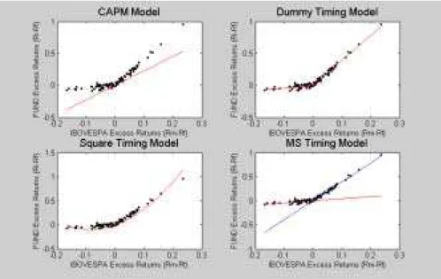
As expected, the estimations of dummy and squared regressors timing mod-els capture manager’s movements very well, and the result is that all modmod-els reject the null hypothesis of one beta and admit the existence of a second one. The difference in interpretations of meanings of the tests is that traditional tests of market timing indicate here success in market timing strategies while theÞxed probabilities MS (MSFP) tests andÞnd support for its existence. Note that the

Þxed and changing probabilities MS models estimates for betas and sigma are quite similar. The LR test for the changing probability MS model (MSCP) rejects the null hypothesis that market return coefficients are null, and market timing efficiency is captured by our model. The graphics of Þgure 2 show the

Þtting of the models used in this study to this data set:

As you can see, all timing models are able to estimate correctly betas on this situation. In this situation, there is no efficiency loss in estimating betas using a MS model. As our discussion is about estimating betas consistently and efficiently, all the things discussed with these two simulations apply to both

Þxed and changing probabilities MS models. We next deal with simulations that have special implications for the changing probabilities model.

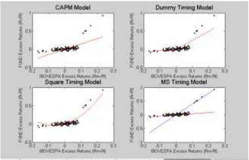
5.3.3 Simulation 3: timing at points other than zero

One of the implicit hypothesis of the Dummy Timing model is that the break even point for the fund manager to change betas of her portfolio is zero excess

Figure 3: timing at points other than zero

returns of the market portfolio. But a manager can adopt the strategy of just changing betas when his expectations of future returns are extremely high (or extremely low). If this happens, the Dummy model will partition the sample erroneously, attributing to a high beta part of the sample observations that in fact belong to the high beta part of the sample. This may contaminate the high beta part of the sample with low beta observations (or vice-versa), making estimates of the higher beta undervalued. The graphics ofÞgure 3 show this idea with data simulated the same way as on simulation 2, except for the fact that the observations that will constitute the higher beta partition of the sample are just the ones correspondent to the 5% higher excess returns of the IBOVESPA over the CDI.

You can see clearly, in the Þgure, that the higher beta is underestimated on the Dummy Timing model. The estimates for the squared regressors timing model is better than the ones obtained by the Dummy approach, but they also underestimate fund returns when true beta is the higher one. As the MS models do not partition the sample, just attribute probabilities to observations coming from one or other part of the sample, the problem just described does not happen with MS estimates.

Table 3

Model: Simul. CAPM Dummy Square MSFP MSCP

θ0₁ - - - 204.00469

θ0₂ - - - -249.44723

θ1₁ - - - -1954.9193

θ1₂ - - - -2450.3924

p11 - - - - 0.92819

-p12 - - - - 0.071809

-p21 - - - - 0.98469

-p22 - - - - 0.015306

-β₁ 0.5 1.4574 0.35084 1.3053 0.40163 0.40465

β₂ 4.0 - 2.45254 9.839 3.9445 3.9487

σ 0.025 0.10764 0.084029 0.06677 0.028172 0.028398

logL - 84.2387 - - 204.8103 222.7717

test stat. - - 8.1651* 12.8959* 241.1432* 35.9228*

test type - - t t LR+ LR+ +

* signiÞcant at 95% percent of signiÞcance

+ _H

0:β1= β2.Test uses the distribution derived by Garcia (1998), p. 773, table

1A.

+ + _H

0:θ11,θ12= 0.Test uses theχ2distribution.

Market timing efficiency is measured on the dummy model as the difference between the two betas. So, in this situation, we obtained a measure of 2.1017 for it. The Square timing measure (β₂) obtained here is 9.839. Our timing measure (TM) for this simulated data is -3.5462e-042. Recall that an individual that manages a fund the way related here is only able to recognize high returns when they are extremely high. As our timing measure is based solely on probability values, it is not surprising that we found a median value for it in this situation. This will be important when we compare the results obtained here with the ones obtained with the next simulated data set, which will treat a situation similar to the one described by simulation 2.

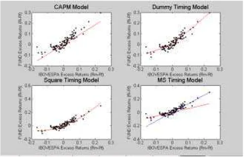
5.3.4 Simulation 4: successful but conservative manager

This simulation retreats a situation where the manager is very successful in market strategies, but for some reason he is conservative, not increasing his exposition to risk very much when expecting high market portfolio returns. The simulation is carried out the same way we did on simulation 2. The only difference is that higher beta value is now lower than in Simulation 2: only 1.25. We plotted the estimates obtained in Þgure 4.

Figure 4: successful but conservative manager

Table 4

Model: Simul. CAPM Dummy Square MSFP MSCP

θ0₁ - - - -240.00404

θ0₂ - - - 69.359674

θ1₁ - - - -5442.9995

θ1₂ - - - 2636.9211

p11 - - - - 0.4655

-p12 - - - - 0.5345

-p21 - - - - 0.45944

-p22 - - - - 0.54056

-β₁ 0.5 0.91633 0.53598 0.87875 0.54923 0.50957

β₂ 1.25 - 1.25838 2.4319 1.2717 1.2599

σ 0.025 0.033016 0.023566 0.025584 0.023534 0.022709

logL - 207.1477 - - 221.6449 246.0354

test stat. - - 10.0074* 8.3186* 28.9944* 48.781*

test type - - t t LR+ LR+ +

* signiÞcant at 95% percent of signiÞcance

+ _H

0:β1= β2.Test uses the distribution derived by Garcia (1998), p. 773, table

1A.

+ + _H

0:θ11,θ12= 0.Test uses theχ2distribution.

the dummy and square timing measures are, respectively, 0.7224 and 2.4319. It means that they are considerably lower than the ones obtained in simulation 3. It happens because, despite the fact that simulated manager 4 usually antici-pates correctly future returns, while manager 3 only seldom does it, the returns obtained by manager 3 by a higher risk exposition are much greater than those obtained by manager 4 because of the relative conservativeness of manager 4. An investor, however, may want to know how many future returns managers can anticipate rather than the return they obtain in one or two observations, as the situation described by simulation 3, because this isolated returns may reßect abnormal situations that may not repeat in the future, what is usually investors’ actual interest. Our MSCP timing measure obtained for this data set is 6.6613e-016. Note that this is a little bit higher than the one obtained for simulation 3 data set. This reßects manager 4’s greater ability in anticipating future returns, despite her conservativeness. If one wants to obtain a measure that gives information similar to those given by traditional measures, all he has to do is to multiply this measure by the differences of betas, and she will obtain the desired information.

5.3.5 Simulation 5: Continuous market timing

Here we simulate data where we can interpret market timing strategies as being continuous, in the sense of a higher expected return will imply in a higher risk position. We generate our data as if fund manager changed betas proportion-ally to his expectation of future returns and is well succeeded in doing it. An extremely high return of the market portfolio will then be associated with an abnormally high beta while a high but not extraordinary one will be associated with a high beta but not as high as in the other case. This kind of situa-tion could be modeled with betas varying according to market excess returns. Imagine that CAPM betas vary linearly with market excess returns:

β_i= ζ_i+ η_iE[Rmt−Rf t] (17)

Sustituting it on the CAPM equation, we obtain:

[Rit−Rf t] = ζi[Rmt−Rf t] + ηi[Rmt−Rf t]2 (18)

This equation is similar to that we used in the Quadratic model described on section 2.2. This suggests that, if managers change continuously betas accord-ing to their expectations and their expectations are usually right, the quadratic model would be the one which captures best this kind of strategy. Here we sim-ulate data that are compatible with this strategy, by adding a disturbance term to equation 18 the same way we did with the other simulated data sets. Note that data generated here depends not only on the excess returns of IBOVESPA but also on its square. Figure 5 shows the data we generated as well as Þtting of the estimated parameters:

Figure 5: Continuous market timing

Table 5

Model: Simul. CAPM Dummy Square MSFP MSCP

θ0₁ - - - -286.38724

θ0₂ - - - -78.231308

θ1₁ - - - -6072.9481

θ1₂ - - - 3244.6222

p11 - - - - 0.61484

-p12 - - - - 0.38516

-p21 - - - - 0.61705

-p22 - - - - 0.38295

-β₁ 0.5 0.60648 0.13639 0.54552 0.17555 0.076308

β₂ 4.0 - 1.02468 3.7888 1.1686 1.0384

σ 0.025 0.040412 0.028715 0.024 0.025272 0.026285

logL - 186.1274 - - 213.084 230.8107

test stat. - - 10.0988* 13.8161* 53.9132* 35.4534*

test type - - t t LR+ LR+ +

* signiÞcant at 95% percent of signiÞcance

+ _H

0:β1= β2.Test uses the distribution derived by Garcia (1998), p. 773, table

1A.

+ + _H

0:θ11,θ12= 0.Test uses theχ2distribution.

Figure 6: successful market timing with some errors

disadvantage of the square model: if there are errors in predictions of the fu-ture, it will not capture them, while the MS models will, as shown with data of simulation 1 data set.

5.3.6 Simulation 6: successful market timing with some errors

Along this section, we have been simulating data as if the true data genera-tion process was one in accordance to one of the existent models or a slight modeiÞcation on them (square timing on simulation 5 and and dummy timing on simulations 2, 3 and 4). Now we are going to generate data as if the true DGP was one in accordance to our MSCP model. First of all, note that we can generate data similar to those of simulations 1 to 4 with this model. For simulation 1, if we set all beta and sigma parameters the same way and set θ1 = θ2 =

£

0 0 ¤, adding a disturbance term in the end, we will obtain a data set similar to simulation 1 data set. For simulation 2, arbitrarily high values forθ1₂and low ones forθ1₁ generate simlar data sets to simulation 2 (let’s say, for example,θ1=

£

0 −100 ¤andθ2 =

£

0 100 ¤). Data set similar to simulation 3 can be generated withθ1=

£

10 −100 ¤andθ2=

£

−10 100 ¤. Simulation 4 can be obtained the same way we did for simulation 2. An inter-esting case is where there is relative success in market timing strategies, but these strategies fail sometimes. We expect that traditional measures of market timing may underestimate actual beta differences. For that purpose, we simu-lated data with the same beta and sigma parameters as in simulation one and theta parameter values ofθ1=

£

0 −30 ¤andθ2=

£

0 30 ¤. Figure 6 plots simulated data as well as model estimations:

Table 6

Model: Simul. CAPM Dummy Square MSFP MSCP

θ0₁ 0 - - - - -0.270194

θ0₂ 0 - - - - 0.779521

θ1₁ -30 - - - - -28.9713

θ1₂ 30 - - - - 27.2185

p11 - - - - 0.30202

-p12 - - - - 0.69798

-p21 - - - - 0.50667

-p22 - - - - 0.49333

-β₁ 0.5 2.4331 1.0007 2.27242 0.54733 0.5199

β₂ 4.0 - 2.7206 10.3968 3.9707 4.0195

σ 0.025 0.11178 0.070066 0.067334 0.023986 0.022728

logL - 80.3203 - - 189.6498 210.7252

test stat. - - 12.676* 13.5129* 109.3295* 42.1508*

test type - - t t LR+ LR+ +

* signiÞcant at 95% percent of signiÞcance

+ _H

0:β1= β2.Test uses the distribution derived by Garcia (1998), p. 773, table

1A.

+ + _H

0:θ11,θ12= 0.Test uses theχ2distribution.

All the models are able to identify market timing. MS models identify ei-ther the existence and success of market timing. The beta diferences, however, are underestimated by the dummy and quadratic market timing models. As disturbance variance is greater for these models when compared to MS models, it is straightforward that these models ignore important information that MS models do not neglect.

5.4

Estimation Results

At this subsection, we will display results obtained from estimating model pa-rameters with real world data. This data set is the one described on the Data subsection. Along earlier pages,we have described two models: a MS model with Þxed probabilities and a MS model with changing probabilities. We will display parameter estimates for these two models. After that, using parameters estimated, we will calculate the timing measures (TM) as given by equation 16. These TM values will be used then to rank the funds of our database. The same procedure will then be carried out to the traditional market timing measures discussed in Section 2. We will then compare rankings obtained using these methods and then see whether they coincide or not.

5.4.1 Fixed probabilities model estimates

Table 7

Funds E quity p11 p21 p12 p22 Beta1 Beta2 Sigma logL LR

BB-ACOE S CARTE IRA LIVRE 1 3820.17 0.99 0.47 0.01 0.53 0.156 1.02 0.01 359.40 30.73 *

BB CARTE IRA ATIVA 1906.47 0.90 0.90 0.10 0.10 -1.066 -0.01 0.01 374.32 67.10 *

DYNAMO PUMA 485.64 0.23 0.16 0.77 0.84 -0.826 0.29 0.02 277.68 9.01

OPPORTUNITY LOGICA II FIA 449.47 0.98 0.41 0.02 0.59 0.775 2.66 0.04 189.92 31.95 * BB-ACOE S PRICE 357.75 0.51 0.50 0.49 0.50 -0.037 0.03 0.00 418.14 2.59

BB-GUANABARA 306.68 0.53 0.01 0.47 0.99 1.020 5.00 0.04 188.41 22.91 *

ITAUACOE S - FIA 272.45 0.94 0.73 0.06 0.27 0.685 1.48 0.02 257.59 20.76 *

BRASIL PRIVATE E QUITY 234.24 0.59 0.59 0.41 0.41 0.106 0.11 0.03 208.66 0.00

CITIACOE S 191.47 0.99 1.00 0.01 0.00 1.021 2.65 0.02 262.29 12.81 * BRADE SCO FIA 170.93 0.08 0.08 0.92 0.92 0.798 14.85 0.02 261.86 35.50 *

* signiÞcant at 95% percent of signiÞcance

H0:β1= β2.Test uses the distribution derived by Garcia (1998), p. 773, table 1A.

We accept the null hypothesis of existence of only one beta for seven of the ten greatest Brazilian stock funds. Of course this is a very high percentage. This may happen due to the following factors: the fund manager adopts in fact passive strategies on a benchmark other than IBOVESPA. In this case, if the portfolio of this benchmark for some reason (redeÞnitions of portfolios of either the benchmark or IBOVESPA, for example) behaves as if it was a market timing managed fund, all passive funds that use this benchmark as its own will present market timing behavior. Another reason is that using Garcia’s distribution on our LR test may in fact not reßect a 95% level of conÞdence, as the variance of the distributions of our LR statistic may be greater on our case than on Garcia’s. It means that the critical value of the LR statistic might be greater than the one we used. As these topics are not on the center of our discussion, we will leave them aside.

Abstracting from these statistical problems, if we analyze our whole data base, we will see that, from the complete data base of 206 funds, 154 have some kind of market timing strategy. This is much higher than our common sense would tell us, as many of these funds have some benchmark to follow strictly, what would lead us to think of these funds as passive and, therefore, not managed by market timers.

5.4.2 Changing probabilities model estimates

parameters of the model for the 206 mutual stock funds in our database. The results for the complete database are shown in the appendix. Table 8 shows the results we found for the top ten funds in equity value:

Table 8

Funds E quity theta01 theta11 theta02 theta12 Beta1 Beta2 Sigma logL LR BB-ACOE S CARTE IRA LIVRE 1 3820.17 211.35 -3089.46 4.57 1.7 1.02 0.16 0.007 360.80 2.53

BB CARTE IRA ATIVA 1906.47 -34.51 57.82 3.87 -5.61 -1.07 -0.01 0.006 374.38 0.27

DYNAMO PUMA 485.64 35.2 27.3 -114.92 141.7 0.29 -0.83 0.017 278.17 1.78

OPPORTUNITY LOGICA II FIA 449.47 4.00 -0.32 -234.37 3887.5 0.78 2.67 0.037 190.94 2.09

BB-ACOE S PRICE 357.75 -15 2985 26.45 -4235.5 -0.06 0.05 0.003 461.83 87.85 *

BB-GUANABARA 306.68 4.55 1.53 211.23 -3090.2 1.02 5.00 0.037 189.83 1.88

ITAUACOES - FIA 272.45 3.03 -0.04 -0.42 0.00 0.69 1.49 0.018 257.59 0.01 BRASIL PRIVATE E QUITY 234.24 4.69 9.35 -29.95 -3.05 0.13 -7.54 0.015 286.27 0.31

CITIACOE S 191.47 1.77 -5.5 3.78 12.64 1.36 0.95 0.018 263.14 0.26

BRADESCO FIA 170.93 4.61 2.42 -33.89 40.34 0.80 14.85 0.018 262.75 4.83

* signiÞcant at 95% percent of signiÞcance

H0:θ11,θ 1

2= 0.Test uses theχ2distribution.

Note that only one of the ten greatest stock funds have transition proba-bilities signiÞcantly related to market returns. It means that only one fund may have succeeded on market timing strategies: BB-Ações Price. As we ac-cepted the null hypothesis of only one beta for BB-Ações Price, it means that no market timing strategies are employed by this fund. So none of these funds is candidate for a well succeeded market timing management. We can also use our Timing Measure in order to evaluate if they are well succeeded funds. Recall that our chosen low (L) and high (H) values of the IBOVESPA return were

RL

m= Rm−2s(Rm) andRHm= Rm+ 2s(Rm), respectively.

Table 9

Funds E quity p11(L) p22(L) p11(H) p22(H) TM

BB-ACOE S CARTE IRA LIVRE 1 3820.17 0.987 1.000 0.992 0.000 -0.502

BB CARTE IRA ATIVA 1906.47 0.000 0.990 0.000 0.958 -0.016

DYNAMO PUMA 485.64 0.000 1.000 0.000 1.000 0.000 OPPORTUNITY LOGICA II FIA 449.47 0.983 0.000 0.981 1.000 0.501

BB-ACOES PRICE 357.75 0.000 1.000 1.000 0.000 -1.000

BB-GUANABARA 306.68 0.987 1.000 0.991 0.000 -0.502

ITAUACOES - FIA 272.45 0.954 0.396 0.954 0.396 0.000

BRASIL PRIVATE E QUITY 234.24 0.000 0.971 0.000 0.997 0.013

CITIACOES 191.47 0.897 0.922 0.996 0.742 -0.139 BRADESCO FIA 170.93 0.987 0.000 0.993 0.000 -0.003

successful timers, as we cannot reject the null hypothesis that there is no antic-ipation. The same thing done here was done to all the funds of our database. The results are displayed at the appendix. From the 206 total stock funds, 154 have passed the market timing existence LR test but only 23 have passed the LR test for efficiency. From these total, 11 funds have passed both tests and, from these, only 2 have positive timing measures (Caixa Ações and Unibanco Galileu - CL). It means that, from the total of 206 funds, only two can be considered somehow statistically successful market timers. This means that, if we look at the fund industry as a whole, we can say that market timing strategies do not work considerably well, as we cannot reject the hypothesis that any success a manger obtained is only due to good luck.

5.4.3 Comparison between models’ estimates

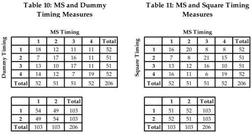
After estimating our models’ parameters and outlining the results above, we estimated the parameters of dummy and quadratic regression timing models and compared the ranking resulted from these estimates with the ones generated by our Timing Measure. The results for the MS parameter estimates are all shown at the appendix. To make this comparison, we partition our sample in two and in four subsamples and verify whether a fund positioned at one partition of the sample according to a traditional way of estimating market timing stays at the same partition in our ranking. We then build two matrices relating each fund to its quartile and above/below median positions on both ours and a traditional market timing measure. The number on the i-th row and j-th column of this matrix represent the number of funds that are simultaneously at thei-th quartile on the traditional timing measure distribution andj-th quartile on MS timing measure distribution. The results are displayed on Tables 10 and 11.

1 2 3 4 Total 1 2 3 4 Total

1 18 12 11 11 52 1 16 20 8 8 52

2 7 17 16 11 51 2 7 8 21 15 51

3 13 10 17 11 51 3 13 12 16 10 51

4 14 12 7 19 52 4 16 11 6 19 52

Total 52 51 51 52 206 Total 52 51 51 52 206

1 2 Total 1 2 Total

1 54 49 103 1 51 52 103

2 49 54 103 2 52 51 103

Total 103 103 206 Total 103 103 206

D

u

m

m

y

T

im

in

g

MS Timing

S

q

u

a

re

T

im

in

g

Table 10: MS and Dummy Timing Measures

Table 11: MS and Square Timing Measures

MS Timing

high numbers at the whole principal diagonal: 18, 17, 17 and 19. Outside the main diagonal, the numbers are lower. Summing the elements of the principal diagonal we obtain 71, a value considerably higher than the expected 51.5. Analyzing the above/below median matrix, we see that a fund that is above the median value according to the Dummy approach has a little more probability of being above median according to the MS approach than below it. These results suggest that the rankings obtained by the two approaches have similarities. Similar results are obtained comparing rankings obtained with MS and Squared approaches. The sum of the principal diagonal of the quartile matrix is greater than 51.5 (it sums 59). Analyzing the above/below median matrix, we see that a fund that is above the median value according to the Square approach has about the same probability of being above median according to the MS approach than below it. Therefore, market timing rankings obtained with MS and Squared Regressors approaches are far from equal, but have some similarities.

The reasons for the differences of the MS and traditional rankings for timing have already been discussed along earlier sections. The MS timing measure is based solely on probabilities, while traditional ones are based on leverage. The MS measure developed here tells us which managers were the best predictors of future returns. The traditional ones tell us which managers have taken more advantage of the opportunities occurred. The advantage of the MS is that it is less sensible to an extremely abnormal return obtained by the fund. If someone wants to obtain an information that has an interpretation similar to traditional ones, all she has to do is multiply TM by the difference in betas.

6

Conclusion

For mutual funds investors, it’s important to have information about how the funds in which they might invest are managed. Some are managed passively and some actively. One way mutual funds are possibly actively managed is through market timing strategy, the practice of changing portfolio betas ac-cording to the expectancy of market behavior. The models commonly used to extract the information of how well done is the market timing strategy under-estimates beta differences by taking observed behavior of market instead of the unobserved manager’s expectancy of market behavior. We proposed an alter-native approach to estimate market timing betas by using Markov switching coefficients in a CAPM framework, which we have estimated using maximum likelihood numerical methods. This approach allows us to test for the existence of market timing strategies in a fund’s management. The only problem with this test is that the LR statistic asymptotic distribution is not the same as in usual LR tests. This asymptotic distribution will be data dependent, so it will be impossible to derive a distribution that can be used with any database. The distribution we used to carry out our hypotheses tests was provided by Garcia (1998) to a MS model with switching on the mean level of the variable. This approximation may underestimate the variance of the LR and, consequently, the critical value of LR, meaning that we will reject the null hypothesis more than we want to.

in which transition probabilities are functions of market portfolio returns. The idea is that if managers can correctly anticipate future states of nature, the transition probabilities will be then correlated with future returns. Based on parameter estimates of this model, we construct a timing measure and, with the information it gives plus a traditional LR test, we are able to say whether the manager is a well succeeded market timer or not. Simulations showed that this model may be quite successful in detecting market timing success for some situations. For others, as that speciÞed by simulation 2, the LR test may fail. If someone believes this kind of situation is common, a dummy variable term can be added in the logit equations for transition probabilities to take this effect into account. This approach was successful for the simulated data sets 2, 3 and 4, as seen on Table 6.

The estimations we made for Brazilian stock mutual funds data lead us to the colclusion that Brazilian fund managers were not considerably successful in their market timing strategies. This result is similar to those obtained by Mazali, Simonsen and Basílio (2000) using the dummy approach to market timing and, observing the results we obtained with traditional models would lead us to similar conclusions. What is surprising is that, despite this fact, many managers did try to be successful market timers, as the results we obtained for the LR test of the number of states of nature suggest. This result could be weakened by the fact that the LR distribution we used to derive critical values may not be appropriated and the true distribution may give us considerably higher ones and by the fact that we used IBOVESPA as the benchmark for the whole industry when it is clearly not true.

Comparing rankings according to MS model and traditional ones using real world data, we observe important differences. These differences are expected since the interpretations of traditional timing measures and MS ones are not the same. The results, however, are not that different, maintaining many similarities between them, as can be seen on Tables 10 and 11. The main limitation of this measure is the lack of a distribution for the LR existence test statistic, what can lead us to reject the null hypothesis more than we want to, if we use Garcia’s distribution as an approximation of the true distribution.

References

[1] Dempster, A. P., N.M. Laird and D.B. Rubin (1977) ”Maximum Likeli-hood from Incomplete Data via the EM algorithm” Journal of the Royal Statistical Society Series B, 39:1-39.

[2] Diebold, F. X., J. H. Lee and G. C. Weinbach (1996) ”Regime switching with time-varying probabilities”, in Hargreaves, C. ”Non-stationary Time Series Analysis end Cointegration” Oxford University Press, London.

[3] Garcia, R. (1998) ”Asymptotic Null Distribution of the Likelihood Ratio Test in Markov Switching Models”,I nternational Economic Review, 39(3), 763-788.

[5] Hamilton, J. D. (1990) ”Analysis of Time Series Subject to Changes in Regime”Journal of Econometrics, 45, 39-70.

[6] Hamilton, J. D. (1994) ”Time Series Analysis” Princeton University Press, Princeton.

[7] Hansen, B. (1991) ”Inference when a nuisance parameter is not identiÞed under the null hypothesis” Working Paper No. 296, Center for Economic Research, University of Rochester.

[8] Hansen, B. (1992) ”The Likelihood Ratio Test Under Non-Standard condi-tions: Test Markov-Switching Model of GNP”Journal of Applied Econo-metrics, 7, S61-S82.

[9] Hansen, B. (1996) ”Inference when a nuisance parameter is not identiÞed under the null hypothesis”Econometrica, 64, 413-30.

[10] Henriksson, R. D. and R. C. Merton (1981) ”On the market timing and investment performance: ii. statistical procedures for evaluation forecasting skill”Journal of Business54(4), 513-533.

[11] Lakonishok, J. A. Schleifer and R. Vishny ”The Structure and performance of the money management industry” Brookings Papers on Economic Ac-tivity, Microeconomics, 1992, pgs. 339 a 391.

[12] Lee, L.-F., A. Chescher (1986) ”SpeciÞcation Testing When Score Test Statistics is Identically Zero”Journal of Econometrics, 31, 121-149.

[13] Mazali, R., R. Simonsen and P. L. A. Basílio (2000). ”Market Timing”.

Conjuntura Econômica, Rio de Janeiro, 54(6), 56-57.

[14] Merton, R. C. (1981) ”On market timing and investment performance: i. an equilibrium theory of value for market forecasts” Journal of Business, 54(3), 363-406.

[15] Kon, S. J. and F. C. Jen (1978) ”Estimation of time-varying systematic risk and performance for mutual fund portfolios: an application of switching regression,Journal of Finance33(2), 457-475.

[16] Nelder, J.A. and R. Mead (1965), ”A Simplex Method for Function Mini-mization,”Computer Journal, 7, 308-313.

[17] Quandt, R. E. (1972) ”A new approach to estimate switching regressions”

Journal of the American Statistical Association, 67 (338), 306-310.

[18] Sharpe, W. (1964) ”Capital Asset Prices: A Theory of Market Equilibrium under Conditions of Risk”Journal of Finance, 19, 425-442.

[19] Sharpe, W., Alexander, G. and Bailey, J. (1991) ”Investments” Prentice Hall, Upper Saddle River.

St at ist ical Appendix

St at ist ical Appendix

St at ist ical Appendix

St at ist ical Appendix