Comparison of region-of-influence methods for estimating high quantiles of precipitation in a dense dataset in the Czech Republic

www.hydrol-earth-syst-sci.net/13/2203/2009/ © Author(s) 2009. This work is distributed under the Creative Commons Attribution 3.0 License.

Earth System

Sciences

Comparison of region-of-influence methods for estimating high

quantiles of precipitation in a dense dataset in the Czech Republic

L. Ga´al1,2and J. Kysel´y1

1_{Institute of Atmospheric Physics, Academy of Sciences of the Czech Republic, Bocn´ı II 1401,ˇ}

141 31 Prague 4, Czech Republic

2_{Department of Land and Water Resources Management, Faculty of Civil Engineering, Slovak University of Technology,}

Radlinsk´eho 11, 813 68 Bratislava, Slovakia

Received: 16 December 2008 – Published in Hydrol. Earth Syst. Sci. Discuss.: 14 January 2009 Revised: 21 August 2009 – Accepted: 2 September 2009 – Published: 20 November 2009

Abstract. In this paper, we implement the

region-of-influence (ROI) approach for modelling probabilities of heavy 1-day and 5-day precipitation amounts in the Czech Republic. The pooling groups are constructed according to (i) the regional homogeneity criterion (assessed by a built-in regional homogeneity test), which requires that in a pooling group the distributions of extremes are identical after scaling by the at-site mean; and (ii) the 5T rule, which sets the min-imum number of stations to be included in a pooling group for estimation of a quantile corresponding to return period T. The similarity of sites is evaluated in terms of climato-logical and geographical site characteristics. We carry out a series of sensitivity analyses by means of Monte Carlo sim-ulations in order to explore the importance of the individual site attributes, including hybrid pooling schemes that com-bine both types of the site attributes with different relative weights.

We conclude that in a dense network of precipitation stations in the Czech Republic (on average 1 station in a square of about 20×20 km), the actual distance between the sites plays the most important role in determining the similarity of probability distributions of heavy precipitation. There are, however, differences between the optimum pool-ing schemes dependpool-ing on the duration of the precipitation events. While in the case of 1-day precipitation amounts the pooling scheme based on the geographical proximity of sites outperforms all hybrid schemes, for multi-day amounts the inclusion of climatological site characteristics (although with much lower weights compared to the geographical distance) enhances the performance of the pooling schemes. This find-ing is in agreement with the climatological expectation since multi-day heavy precipitation events are more closely linked

Correspondence to:L. Ga´al ([email protected])

to some typical precipitation patterns over central Europe (re-lated e.g. to the varied roles of Atlantic and Mediterranean influences) while the dependence of 1-day extremes on cli-matological characteristics such as mean annual precipitation is much weaker.

The findings of the paper show a promising perspective for an application of the ROI methodology in evaluating outputs of regional climate models with high resolution: the pool-ing schemes might serve for definpool-ing weightpool-ing functions, and the large spatial variability in the grid-box estimates of high quantiles of precipitation amounts may efficiently be re-duced.

1 Introduction

Advantages of regional frequency models over the at-site approach (which utilizes data from the site of interest only) stem from the reduced uncertainty of the estimated high quantiles at the upper tails of the distributions (e.g. Letten-maier et al., 1987; Cunnane, 1988; Stedinger et al., 1993) and the fact that the regional methods allow for the estima-tion of design values at ungauged locaestima-tions (e.g. GREHYS 1996a, b; Kohnov´a et al., 2006).

In the traditional approach to regional frequency analy-sis, the regions are kept fixed. That is to say, when chang-ing the focus from one site to another within a given region, the information source for the regional transfer remains un-changed (e.g. Hosking and Wallis, 1997). An alternative to regional frequency estimation, the region-of-influence (ROI) approach (Burn, 1990a, b) introduced a fundamentally differ-ent concept: the idea of focused pooling. Its main feature is the uniqueness of the “regions” (more precisely, the pooling groups – Reed et al., 1999b), wherein each site under study has its own group of adequately similar sites that form the basis for the transfer of information on extremes to the site of interest. The idea of focused pooling has been adopted in studies of flood flows (e.g. Zrinji and Burn, 1994, 1996; Castellarin et al., 2001; Cunderlik and Burn, 2002; Holmes et al., 2002; Shu and Burn, 2004) and precipitation extremes (Schaefer, 1990; Alila, 1999; Di Baldassare et al., 2006), as well as in complex nationwide projects devoted to the fre-quency analysis of hydro-climatological extremes (Reed et al., 1999a; Thompson, 2002).

In an analysis of extreme precipitation amounts in Slo-vakia, Ga´al et al. (2008a) adopted the original concept of the ROI approach (Burn, 1990b) even though the fact that Burn’s original methodology had previously been subjected to crit-icism due to the need to set a relatively large number of pa-rameters according to subjective considerations (e.g. Hosk-ing and Wallis, 1997). Zrinji and Burn (1994) revisited the ROI methodology: instead of subjectively selected thresh-old values, they used a built-in regional homogeneity test based on theχ_R2 statistics (Chowdhury et al., 1991) for as-signing sites to a given pooling group. Later, Zrinji and Burn (1996) extended the ROI methodology by a hierarchical feature (Gabriele and Arnell, 1991) that implemented sev-eral alternatives to the homogeneity test of Hosking and Wal-lis (1993). Castellarin et al. (2001) applied the hierarchical pooling methodology of Zrinji and Burn (1996) for a flood frequency analysis in north-central Italy.

The present study attempts to overcome some shortcom-ings of the methodology applied in Ga´al et al. (2008a), par-ticularly with respect to the subjective decisions made in the process of forming the pooling groups. For that pur-pose, a test of regional homogeneity is incorporated. Further improvements include a detailed sensitivity analysis which examines the performance of various ROI pooling schemes by means of simulation experiments: in addition to those schemes based purely on climatological or geographical site attributes, hybrid pooling schemes are constructed and

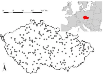
com-Fig. 1. 209 climatological stations available for a regional fre-quency analysis of heavy precipitation amounts in the Czech Re-public.

pared. The performance of the ROI methodology for mod-elling probabilities of extreme 1-day and multi-day precipi-tation amounts is evaluated using data from a dense network of rain gauges in the Czech Republic.

2 Data

2.1 Precipitation data

Daily precipitation totals measured at 209 stations mostly op-erated by the Czech Hydrometeorological Institute (CHMI) were used as the input dataset (Fig. 1). The altitudes of the stations range from 150 to 1490 m a.s.l., and the observations at most sites span the period from 1961 to 2005. Three main criteria were applied when selecting the stations and forming the dataset:

1. spatial coverage – the stations about evenly cover the territory of the Czech Republic,

2. relocations of stations – no significant station moves during 1961–2005 (all sites where any location changes exceeded 50 m in altitude were excluded from the analysis), and

The dataset is superior to the one employed in Kysel´y and Picek (2007a), especially since it involves a much larger number of sites with complete daily records, more evenly covers the territory of the Czech Republic, and extends to the very recent past (December 2005). Furthermore, a few errors were identified in the original dataset and have been corrected.

At 45 stations, minor gaps in the daily records occurred (a total of up to 1 month over 45 years at 32 sites; not exceed-ing 3 months at any of the 45 sites). We decided to preserve these stations in the analysis because of their locations in ar-eas that are insufficiently covered by rain gauges with com-plete records. The missing daily data were estimated using measurements at 2 to 5 nearest locations available in the cli-matological database of the CHMI; the methodology is de-scribed in Kysel´y (2008). (Note that the mean distance to the nearest measuring site was 15.4 km for the locations where the missing data were estimated, and the percentage of the missing daily records in the entire dataset was only 0.05%.) All other station records with more than 3 months of missing values were excluded from the analysis.

Samples of annual maxima of 1-day and 5-day precipita-tion amounts were drawn from each staprecipita-tion record and are further examined. The percentage of stations with a trend significant at the 0.05 level is low and close to the nominal value for both characteristics, so the data do not violate the assumption of stationarity.

Basic features of the precipitation regime of the Czech Re-public, with a focus on extremes, may be found in Kysel´y and Picek (2007a) and Kysel´y (2008).

2.2 Pooling attributes

The ROI approach is one of the methods of focused pooling and aims at finding groups of sites that share similar statisti-cal properties of the observed hydro-climatologistatisti-cal extremes. It is assumed that the frequency distribution of extremes at a given site is related to its climatological, hydrological, geo-graphical, geomorphological or similar attributes. Therefore, one of the basic issues of the pooling procedure is to select site attributes that are useful for explaining the observed dis-tributions of extremes.

In this study, the similarity of sites is evaluated during the pooling process using two different sets of site attributes. The first group of site attributes consists ofgeneral climato-logical characteristicsthat describe a long-term precipitation regime:

1. mean annual precipitation (MAP),

2. mean ratio of the precipitation totals for warm/cold seasons (RWC), and

3. mean annual number of dry days (DRY), defined as days with precipitation amount≤0.1 mm.

The warm (cold) season is defined as April–September (October–March). The basic idea of choosing characteristics of the precipitation regime is that the atmospheric mecha-nisms generating heavy precipitation are similar under simi-lar climatological conditions, particusimi-larly when the small ex-tent of the study area is taken into account.

Geographical site characteristics comprise the second group of attributes that are employed to define the sites’ prox-imity:

1. latitude (φ), 2. longitude (λ), and

3. elevation above sea level (h).

The geographical co-ordinates are chosen since the actual proximity of the sites may also result in similar regimes of extreme precipitation.

3 Methods

3.1 Concepts of pooling

Since the pooling scheme adopted herein originates from that described in detail in Ga´al et al. (2008a), we confine the de-scription to the cornerstones of the procedure and accentuate the changes and improvements in the methodology.

The similarity of sites in the attribute space is usually eval-uated by means of a weighted Euclidean distance metric:

Dij=

" _M X

m=1

Wm Yim−Yj m2

#12

(1)

whereDij is the weighted Euclidean distance between sites iandj; Wm is the weight associated with them-th site at-tribute, expressing its relative importance;Yimis the value of them-th attribute at sitei; andMis the number of attributes. However, we slightly modified this formula in the following way:

Dij=

"

WGG2ij+ M

X

m=1

Wm Yim−Yj m

2 #1₂

(2)

whereGij is the actual geographical distance between sites i andj, and WG is its weighting coefficient. Gij is deter-mined according to the relationship for the distance between pairs of points [ϕi,λi] andϕj,λjon the surface of a sphere (Weisstein, 2002a):

Gij₌Rarccossinϕisinϕj₊cosϕicosϕjcos λi₋λj (3) whereRdenotes the Earth’s radius (R=6371 km).

due to different magnitudes. In this study, the attributes (ex-cept for the latitude and longitude) were divided by their sample standard deviations while the values ofGij were di-vided by the standard deviation of non-zero elements of the distance matrixG. For settings ofWmandWGsee Sect. 4.2. It is important to point out the difference between two types of the site attributes, which are usually termed “char-acteristics” and “statistics”. Site characteristics are quanti-ties independent of whether or not daily measurements of precipitation are carried out at a given site. These include geographical co-ordinates, geomorphological attributes and, to some extent, descriptors of the long-term precipitation regime. On the other hand, site statistics result from statis-tical processing of the data observed at a given site. It is generally recommended (Hosking and Wallis, 1997; Castel-larin et al., 2001) to use site characteristics in the process of forming the regions or pooling groups, while one should take advantage of site statistics in the process of testing the homogeneity of a proposed group of sites.

Pooling groups in the ROI approach are generally con-structed using elements Dij arranged in ascending or de-scending order, but there are basically two different ways to accomplish this. The core idea of the first method lies in gradually building up the pooling groups (termed herein as the “forward” approach). Starting with the target sitei, which represents a single-site pooling group at the very be-ginning of the process, the next closest site (i.e. the site with the next lowest value ofDij,j₌1,...,N) is appended to the existing ROI in each turn as long as a given condition for forming the ROI is met. The process of building up the ROI may be terminated (i) at a given point, defined as a function of the selected quantiles of the dissimilarity matrixD(Burn, 1990b); (ii) when the measure of the regional homogeneity of the proposed group of sites reaches or exceeds an unac-ceptable level (Castellarin et al., 2001); or (iii) when the size of the proposed pooling group reaches or exceeds a desired threshold value (Jakob et al., 1999). A reversed procedure (“backward” approach) is adopted in the second method of pooling: in its initial stage, all sites in the analysis are sup-posed to form a “superregion” and, step by step, the most dissimilar sites are removed from the bulk of the sites un-til the remaining group of sites is homogeneous (Zrinji and Burn, 1994).

Point (iii) above is particularly appealing for pooling methodologies such as the ROI since the composition of a site’s pooling group may be accommodated to the target re-turn period. The “5T rule” (Jakob et al., 1999) is one of the most frequently referenced rules of thumb to account for the need of different amounts of information for different target return periods. The 5T rule suggests that one needs 5×T station-years of data for a reliable estimation of a quan-tile corresponding to the return periodT. Considering the fact that the average length of observations at the stations in-volved in the present analysis is∼44 years (see Sect. 2.1), for estimation of the 5-year quantiles the at-site approach is

ac-ceptable, while it is desirable to have at leastNT=2 (12) sites in a pooling group for a reliable estimation of the 10 (100)-year precipitation quantiles.

We implemented the regional homogeneity test of Lu and Stedinger (1992) when forming the pooling groups, and for two reasons: (i) its application is computationally straightfor-ward, and (ii) according to the comparative study of Fill and Stedinger (1995), it is one of the most powerful homogeneity tests. A brief description of Lu and Stedinger’s homogeneity test, also called theX10 test, is given in the Appendix.

We tested both the “forward” and “backward” approaches to forming homogeneous ROIs, and then decided to form them primarily by building them up gradually (i.e. using the “forward” approach). The main deficiency of the “back-ward” procedure was that, in some cases, it tended to pro-duce very large homogeneous pooling groups that did not vary much from site to site. This resulted in undesirable spa-tial smoothing of the estimated quantiles (cf. Castellarin et al., 2001).

Two requirements are imposed on the pooling groups in the present study: they should meet (i) the homogeneity cri-terion, and (ii) the 5T rule. Having only the first criterion, the following simple iteration procedure is applicable: In each step, the next similar site is added to the existing ROI and the homogeneity of the proposed pooling group is tested. If the proposed ROI is homogeneous, then the procedure goes on with the next loop; otherwise (i.e. if heterogeneity is de-tected), the procedure is stopped and the formation of the given ROI is finished. When the 5T rule must be met at the same time, however, the result of the iterative procedure may not be sufficient. Problems may occur when the het-erogeneity is reached relatively early, i.e. after a few (<4–6) iterations, which is not plausible for longer return periods (T=50 years or more). We tried adopting the idea suggested by Castellarin et al. (2001) to stop the iteration procedure when the heterogeneity of the ROI is detected for the second time (instead of the first time), but the number of groups con-sisting of a small number of sites was still large. Therefore, the following scheme is proposed for the pooling procedure in the present study:

– At the very beginning, the ROI of the target site consists of the target number of stationsNT (i.e. it comprises the site itself and theNT₋1 closest sites).

– If the initial pooling group of sizeNT is homogeneous there is no need to start iterations;NT defines the final size of the pooling group.

– In a case when no homogeneous stage is reached by suc-cessively adding sites to the initial ROI, the program code returns to the initial stage withNT sites and starts looking for a homogeneous composition by removing the least similar sites from the pooling group. The first homogeneous stage then defines the final composition of the pooling group for the site.

– In the worst case, when neither the building-up nor the removal procedure leads to a homogeneous stage, the ROI consists of nothing but the target site (i.e. it is a single-site pooling group).

The application of this procedure means that, in contrast to the scheme adopted in Ga´al and Kysel´y (2009), the size of the final pooling groups depends onT.

3.2 Estimation of growth factors and quantiles

For constructing pooled cumulative distribution functions and estimating the precipitation quantiles, the generalized extreme value (GEV) distribution was applied (e.g. Coles, 2001). The GEV distribution is widely used for modelling hydro-climatological extremes (e.g. Alila, 1999; Smithers and Schulze, 2001; Castellarin et al., 2001; Kharin and Zwiers, 2005; Fowler and Ekstr¨om, 2009), and frequency analyses of precipitation extremes have also confirmed its applicability in central Europe (the Czech Republic – Kysel´y and Picek, 2007a; Slovakia – Kohnov´a et al., 2006; Ga´al et al., 2008b).

TheT-year growth factors (i.e. theT-year values of the cu-mulative distribution function of dimensionless data; further-more, the term “growth curve” denotes a set of growth factors for different return periods; cf. Stewart et al., 1999) and pre-cipitation quantiles are estimated using the L-moment-based index storm procedure (Hosking and Wallis, 1997). In the initial step, dimensionless data are calculated by rescaling the original data by the sample meanµj(index storm): xj k₌Xj k

µj

, j₌1,...,N, k₌1,...,nj (4)

where Xj k (xj k) denotes the original (dimensionless or rescaled) data,N is the number of sites, andnj denotes the sample size of thej-th site.

The dimensionless values ofxj k at sitej are then used to compute the sample L-momentsl₁(j ),l₂(j ),. . . and L-moment ratios:

t(j )₌l₂(j ).l(j )₁ (5)

and tr(j )=lr(j )

.

l(j )₂ , r₌3,4,... (6)

wheret(j ) is the sample L-coefficient of variation (L-CV) andtr(j ),r=3,4,... are the sample L-moment ratios at site

j (Hosking, 1990). The case r=3 defines the sample L-skewnesst₃(j ); the L-moment ratios of higher degree (r>3) are not of a practical use herein.

The pooled L-moment ratiost(i)Randt₃(i)Rfor the target siteiare derived from the at-site sample L-moment ratios as their weighted averages:

t(i)R₌ N

P

j₌1

Wijt(j ) N

P

j=1

Wij

(7)

whereWijare the weights associated with thej-th site in the analysis. A relationship analogous to Eq. (7) holds true also fort₃(i)R.

In a traditional regional analysis, based on regions with a fixed structure (e.g. Hosking and Wallis, 1997), the weight-ing coefficientsWijare proportional only to the record length nj for all sitesj within a given region (i.e. sites with longer observations provide more information in the regionally av-eraged statistics). While this concept is also retained in fo-cused pooling, an additional factor, the reciprocal value of the distance metric elementDij, is introduced (Castellarin et al., 2001):

Wij=

(

nj

.

D∗_{ij ∀}j_∈ROIi

0 ∀j /_∈ROIi (8)

where ROIi stands for the region of influence of the sitei, and

D∗_ij=

Dij if Dij6=0

Dij,min if Dij=0 (9)

whereDij,min is the lowest non-zero value of the distance

metric between the target siteiand all other sitesj (Castel-larin et al., 2001). (Note thatDii=0 for j₌i, which would lead toWii=∞ifDij was used in Eq. 8.) Using the recip-rocal value of the distance metric elementDij as the pooled weighting factor is equivalent to assigning higher weights to sites that lie in the proximity of the target site in the attribute space: the smaller isDij for sitej, the greater the amount of information it brings to the procedure for the growth curve estimation at sitei.

The (weighted) pooled L-moment ratiost(i)Randt₃(i)Rare then used to estimate the parameters of the GEV distribution and the pooled growth curve. A quantile corresponding to the return periodT at siteiis calculated as a product of the dimensionlessT-year growth factorx_iT and the index storm µi:

X_iT₌µix_iT (10)

3.3 Framework for the inter-comparison of pooling schemes

The performance of the individual pooling schemes based on different combinations of climatological and geographical site attributes (Sect. 2.2) is assessed by means of Monte Carlo simulation procedures.

The essential issue of the Monte Carlo simulation is the way the unknown parent (or “true”) distribution of the ex-tremes is estimated. We decided to estimate the “true” at-site distribution by adopting a region-of-influence approach in which the similarity of sites is determined according to statistical properties of the at-site data samples of 1-day/5-day precipitation maxima (abbr. ROIsta), as in Castellarin et al. (2001) and Ga´al et al. (2008a). Three site statistics were selected (cf. Burn, 1990b; Ga´al et al., 2008a):

1. the coefficient of variation: cv=σµ, whereµ(σ )is the sample mean (standard deviation);

2. Pearson’s 2nd skewness coefficient: PS=3(µ−m)σ, wheremis the sample median (Weisstein, 2002b); and 3. the 10-year growth factor of precipitation, estimated

us-ing the GEV distribution (x10).

The selected statistics characterize the scale (cv), shape (PS) and location (x10) of the empirical distribution. A pooling scheme based on the site statistics is supposed to result in groups of sites that have a frequency distribution of extremes similar to the target site.

The “reference” ROI pooling group for estimating the “true” growth curve is constructed in a slightly different way than the examined ROI pooling schemes. While in the latter case, the size of the pooling groups is adjusted to the tar-get return period T, the ROI pooling group for estimating the “true” growth curve at a given site is independent of the actual target return period. We require that the size of the pooling groups for constructing the “true” quantiles be about NTref=23, which corresponds to the (sufficiently large)

re-turn period of 200 years according to the 5T rule. The idea behind this approach is that if there is a single “true” (and un-known) distribution for a given site, data used for estimating the “true” quantiles should not depend on the actual target return period. Therefore, the choice of a fixed sizeNTref

al-lows for having the same platform for comparison of the ex-amined pooling schemes. Except for differentNTref(see also

Sect. 4.3, in which the size of pooling groups is discussed), the procedure is the same as described in Sect. 3.1 for the ex-amined ROI pooling schemes (i.e. homogeneity of the ROI is required).

In each loop of the Monte Carlo simulation procedure, samples of annual maxima that resemble the real world (in terms of the actual number of sites, length of the observa-tions, and spatial correlations between the sites) are drawn for each site from the parent GEV distribution, parameters of

which are given by the pooled L-moments according to the ROIsta pooling scheme. Having simulated the at-site sam-ples, the pooling schemes specified in Sect. 4.1 and 4.2 are applied to estimate theT-year growth factors, which are then compared with the “true” ones obtained by the ROIsta pool-ing scheme. The loops of the Monte Carlo simulations are repeated 5000 times.

The different pooling schemes are compared by means of the bias and (primarily) the root mean square error (RMSE) statistics. For a given return periodT,

RMSET=_N1

N

X

i₌1 



1 M

M

X

m₌1 ˆ

x_i,mT ₋x_iT x_iT

!2



1 2

(11)

and BIAST₌1

N N

X

i=1

1 M

M

X

m=1 ˆ

x_i,mT ₋x_iT x_iT

!

(12)

wherei(m) is the index over the sites (repetitions);N (M) is the number of sites (repetitions);x_iT is the “true”T-year growth factor at site i; and x_ˆi,mT is the estimated T-year growth factor at sitei from them-th sample of the Monte Carlo simulation.

The Monte Carlo simulation procedure and some re-lated considerations are described in more detail in Ga´al et al. (2008a, Sect. 4).

4 Results

4.1 Sensitivity analysis

In the first step, a sensitivity analysis was performed to ex-plore the role of different site characteristics and site statistics entering the dissimilarity matrix D(Eq. 1) while consider-ing the weightconsider-ing coefficients as unimportant (Wm=WG=1). The basic ROI schemes were analogous to those used in Ga´al et al. (2008a). The models were based on 3 climato-logical (geographical) site characteristics (Sect. 2.2) and la-belled as ROIcli3 (ROIgeo3), and both were associated with the model ROIsta based on 3 site statistics (ROIsta3) used for estimating the “true” quantiles during the simulation pro-cedures (Sect. 3.3). The sensitivity analysis examined the performance of the ROI models after removing one or two site attributes from the basic ROI pooling scheme (ROIcli3, ROIgeo3) or the “true” frequency model (ROIsta3).

Table 1. Summary of site characteristics and site statistics used

in individual ROI pooling schemes. The sign √ indicates that

the given site characteristic or statistic is included into the pooling scheme.

Climatological Geographical Site statistics site characteristics site characteristics

MAP RWC DRY φ λ h cv PS x10 [mm] [−] [−] [◦] [◦] [m] [−] [−] [−]

Changes

in

the

R

OI

pooling

schemes

ROIcli1a √ ROIcli1b √

ROIcli1c √

ROIcli2a √ √

ROIcli2b √ √

ROIcli2c √ √

ROIcli3 √ √ √

ROIgeo1 √

ROIgeo2 √ √

ROIgeo3 √ √ √

Changes

in

the

“true”

model

ROIsta2a √ √

ROIsta2b √ √

ROIsta2c √ √

ROIsta3 √ √ √

MAP = mean annual precipitation, RWC = mean ratio of the precip-itation totals for warm/cold seasons, DRY = mean annual number

of dry days,φ= latitude,λ= longitude,h= altitude,cv= coefficient

of variation, PS = Pearson’s 2nd skewness coefficient,x10=10-year

growth factor of precipitation.

models is reduced: while the ROIcli alternatives make use of all 6 possible combinations of the 3 available climatolog-ical attributes into singles (labelled as ROIcli1a, b and c) or pairs (labelled as ROIcli2a, b and c), there are no reasons for using other simplified ROIgeo models than those based purely on elevation (ROIgeo1) or the pair of geographical co-ordinates (ROIgeo2). Furthermore, the modified “true” frequency models are based only on pairs of possible combi-nations of the site statistics defined in Sect. 3.3 (labelled as ROIsta2a, b and c) since it is unreasonable to construct “true” models based purely on one statistic. The sensitivity analy-sis was performed for both datasets of the 1-day and 5-day annual maxima.

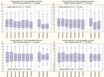
First, we focus on the consequences of the changes made to the basic pooling schemes ROIcli3 and ROIgeo3. The summary statistics of the models’ performance in terms of the average RMSE for the quantiles of the estimated distri-butions of the 1-day (5-day) maxima corresponding toT=10, 20, 50 and 100 years are given in Table 2. The box-and-whisker plots of both statistics in Figs. 2 and 3 illustrate the spread statistics for return periodsT=20 and 100 years.

As expected, the frequency behaviour of the precipita-tion extremes cannot be explained by a single climatological characteristic. This is demonstrated by the fact that the ROI models based purely on a single site attribute show clearly the poorest performance (Figs. 2 and 3). The ROIcli2 mod-els based on two site attributes perform generally better. Of the three models working with the climatological character-istics, the one with MAP and DRY is inferior, which suggests

Fig. 2. Root mean square error (RMSE) and bias of growth

fac-tors corresponding to return periodsT=20 and 100 years for

an-nual maxima of 1-day precipitation amounts in a sensitivity analy-sis when changes made to the basic ROI pooling schemes are ex-amined.

Fig. 3. Root mean square error (RMSE) and bias of growth

fac-tors corresponding to return periodsT=20 and 100 years for

an-nual maxima of 5-day precipitation amounts in a sensitivity analy-sis when changes made to the basic ROI pooling schemes are ex-amined.

Table 2. Performance of the ROI pooling schemes based on different combinations of site characteristics as measures of similarity for

annual maxima of 1-day and 5-day precipitation amounts. RMSET denotes average root mean square error of the estimated growth factors

corresponding to return periodT[years], expressed in %. The smallest values of the statistics are marked in bold, separately for climatological

and geographical characteristics.

Climatological site characteristics Geographical site chars.

T ROI ROI ROI ROI ROI ROI ROI ROI ROI ROI

[yrs] cli1a cli1b cli1c cli2a cli2b cli2c cli3 geo1 geo2 geo3

RMSET[%]: 1-day precipitation amounts

10 3.524 3.573 3.440 3.407 3.406 3.460 3.300 3.456 3.080 3.160

20 6.091 6.085 5.820 5.672 5.828 5.846 5.609 6.090 5.153 5.242

50 9.544 9.557 9.178 8.808 9.078 8.851 8.481 9.491 7.929 8.056

100 12.136 12.166 11.729 11.113 11.332 11.192 10.713 12.323 9.820 10.155

RMSET[%]: 5-day precipitation amounts

10 3.314 3.305 3.238 3.232 3.263 3.134 3.103 3.257 2.991 3.037

20 6.025 5.827 5.741 5.568 5.821 5.403 5.319 5.883 4.997 5.115

50 9.836 9.337 9.470 8.742 9.239 8.519 8.296 9.717 7.404 7.707

100 12.960 12.002 12.336 11.131 11.988 10.761 10.479 12.854 9.109 9.544

Table 3. Performance of the ROI pooling schemes ROIcli3, ROIgeo3 and ROIgeo2 based on different combinations of site statistics in the

“true” frequency model for annual maxima of 1-day and 5-day precipitation amounts. RMSET denotes average root mean square error of

the estimated growth factors corresponding to return periodT [years], expressed in %. The smallest values of the statistics are marked in

bold, separately for the “true” frequency models evaluated.

ROIsta2a ROIsta2b ROIsta2c ROIsta3

T ROI ROI ROI ROI ROI ROI ROI ROI ROI ROI ROI ROI

[yrs] cli3 geo3 geo2 cli3 geo3 geo2 cli3 geo3 geo2 cli3 geo3 geo2

RMSET[%]: 1-day precipitation amounts

10 3.233 3.145 3.054 3.350 3.219 3.126 3.503 3.566 3.476 3.300 3.160 3.080

20 5.622 5.324 5.220 5.710 5.375 5.269 5.932 5.988 5.813 5.609 5.242 5.153

50 8.628 8.212 8.117 8.714 8.372 8.238 9.165 9.262 9.055 8.481 8.056 7.929

100 10.970 10.345 10.039 11.137 10.700 10.327 11.548 11.718 11.480 10.713 10.155 9.820

RMSET[%]: 5-day precipitation amounts

10 3.026 2.974 2.908 3.168 3.114 3.069 3.318 3.321 3.267 3.103 3.037 2.991

20 5.330 5.083 4.965 5.395 5.234 5.099 5.889 5.776 5.702 5.319 5.115 4.997

50 8.491 7.822 7.473 8.397 7.879 7.523 9.443 9.116 9.236 8.296 7.707 7.404

100 10.839 9.751 9.292 10.598 9.767 9.275 12.259 11.573 11.930 10.479 9.544 9.109

While for the ROIcli models more site attributes improve performance, a similar conclusion cannot be drawn for the ROIgeo pooling schemes: the ROIgeo2 model always out-performs the basic ROIgeo3 model, both in terms of the RMSE and bias statistics (Table 2, Figs. 2 and 3). Such be-haviour is accounted for by the role of elevation in ROIgeo3. While in ROIgeo2 sites are pooled according to the geo-graphical distance from the site of interest, ROIgeo3 gives preference to sites that are located in similar altitudes as that of the target site (cf. Fig. 4 and related discussion in Ga´al and Kysel´y, 2009).

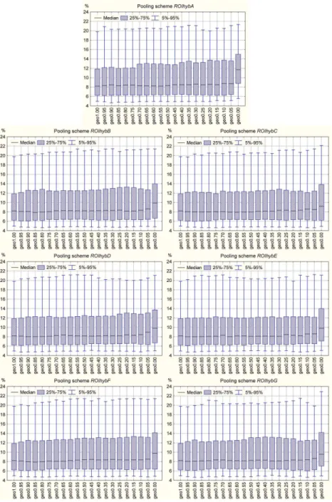
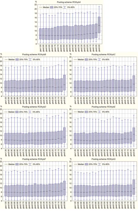
Fig. 4. Root mean square error (RMSE) of growth factors corresponding to return periodT=100 years for annual maxima of 1-day pre-cipitation amounts in a sensitivity analysis when the performance of different series of hybrid pooling schemes (ROIhybA–ROIhybG; see

also Table 4) is compared. The labels of the individual pooling schemes (geo1.00,..., geo0.00) reflect the weighting coefficient for actual

geographical distance between sites (see Sect. 4.2).

model in terms of RMSE (except for high return levels and the ROIsta2c model, which is the inferior one), and both ROIgeo2 and ROIgeo3 pooling schemes perform clearly bet-ter than ROIcli3 (Table 3).

4.2 Hybrid pooling schemes

A further extensive simulation experiment was carried out in order to identify the optimal setting of the ROI pooling

schemes when merging both climatological and geographical site characteristics in hybrid pooling schemes and assigning different weighting coefficients to the selected site attributes of the hybrid pooling schemes.

Table 4.Summary of site characteristics used in hybrid ROI

pool-ing schemes. The sign√indicates that the given site characteristic

is included in the pooling scheme.

Climatological Geographical

site characteristics site characteristics

MAP RWC DRY φ λ h

[mm] [−] [−] [◦] [◦] [m]

ROIhybA √ √ √

ROIhybB √ √ √ √ √ √

ROIhybC √ √ √ √ √

ROIhybD √ √ √ √ √

ROIhybE √ √ √ √

ROIhybF √ √ √ √ √

ROIhybG √ √ √ √

MAP = mean annual precipitation, RWC = mean ratio of the precip-itation totals for warm/cold seasons, DRY = mean annual number of

dry days,φ= latitude,λ= longitude,h= altitude.

scheme ROIhybA is not a hybrid in a strict sense since it only makes use of the geographical site characteristics. Inas-much as the same simulation strategy is applied, however, ROIhybA also is included in this series of experiments. ROI-hybB includes all the 6 site attributes appearing in this study. In the other models, we excluded some of the less important climatological and/or geographical site attributes (based on the results of the sensitivity analysis, Sect. 4.1), which are DRY and MAP on the one hand and elevation on the other.

The weighting coefficients were assigned to the series of the pooling schemes ROIhybA–ROIhybG according to the following considerations: since the geographical distance is an important indicator of sites’ similarity (Sect. 4.1), the weightWGis chosen as the basic parameter. WGtakes val-ues from 1.00 to 0.00 with a constant increment of 0.05. So that the sum of the weights is declared to equal to one, the re-maining value of (1−WG) is evenly distributed between the other site attributes involved in the given series of the pooling schemes. Mathematically:

WG,i₌1.00−i0.05, i=0,...,20 (13) and

Wm,i₌ 1₋WG,i M, i₌0,...,20_;m₌1,...,M (14) where M is the total number of the site attributes other than latitude and longitude (Table 4). The individual pool-ing schemes are therefore labelled as geo1.00, geo0.95,. . . , geo0.00. Note that in each series ROIhybA–ROIhybG, the pooling scheme geo1.00 is the same and corresponds to the ROIgeo2 pooling scheme from Sect. 4.1. Other special cases are the following:

– ROIgeo3 = geo0.50 in ROIhybA,

– ROIcli3 = geo0.00 in ROIhybC,

– ROIcli2a = geo0.00 in ROIhybE, and

– ROIcli2c = geo0.00 in ROIhybG.

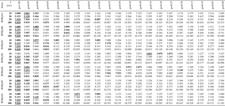
The results of the simulation experiments are summarized in Tables 5 and 6 and Figs. 4 and 5. The box plots are shown for the 100-year quantiles only since the results are similar for shorter return periods.

For 1-day precipitation amounts, the average values of RMSE in Table 5 as well as the median and inter-quartile range (75%–25% percentiles) in Fig. 4 show an increasing tendency from left to right (i.e. the error in the quantile es-timates increases with decreasing weight put onto the geo-graphical distance). For 5-day precipitation amounts (Fig. 5), this feature is superimposed by local minima (characterized by the lowest values of median and the narrowest boxes) around pooling schemes geo0.80–geo0.70, depending on the site attributes involved in a given hybrid scheme. A pattern similar to that of the box plots (Figs. 4 and 5) is also found in terms of the average RMSE values (Tables 5 and 6). In the case of 1-day precipitation maxima, the pooling schemes with the lowest RMSE statistics, for all return periods, are located at the very left side of the table while for 5-day max-ima the best pooling schemes are more scattered. The most remarkable result is that for the ROIhybC series: the model geo1.00 loses its superiority, and the best performance is re-lated to pooling schemes utilizing in addition climatological characteristics (geo0.85–geo0.80).

We conclude that (i) for 1-day precipitation maxima, there is no hybrid pooling scheme that outperforms the pooling scheme ROIgeo2 (i.e. geo1.00 in each series ROIhybA– ROIhybG) based on the actual geographical distance be-tween sites, while (ii) for 5-day precipitation maxima, a few hybrid pooling schemes with performance superior to the ROIgeo2 model in terms of the RMSE statistic can be constructed (ROIhybC: geo0.80 and geo0.95, ROIhybG: geo0.85 and geo0.95). The best of these hybrid pooling schemes (i.e. the one with the lowest RMSE values) is ROIhybC-geo0.80, which utilizes all three climatological site characteristics with equal weights 1/15, and the geo-graphical distance between sites with a weighting factor of 12/15.

4.3 Inter-comparison of the frequency models

Table 5.Performance of the hybrid ROI pooling schemes based on different combinations of climatological and geographical site

charac-teristics for annual maxima of 1-day precipitation amounts. RMSET denotes average root mean square error of the estimated growth factors

corresponding to return periodT [years], expressed in %. The three smallest values of the statistics are marked in bold, and the smallest

value is underlined. The heading shows the weighting coefficient for actual geographical distance between sites. The settings of the series of individual pooling schemes are summarized in Table 4.

Series

T

geo1.00 geo0.95 geo0.90 geo0.85 geo0.80 geo0.75 geo0.70 geo0.65 geo0.60 geo0.55 geo0.50 geo0.45 geo0.40 geo0.35 geo0.30 geo0.25 geo0.20 geo0.15 geo0.10 geo0.05 geo0.00

[yrs]

R

OIh

ybA

10 3.080 3.065 3.103 3.126 3.154 3.169 3.158 3.163 3.162 3.140 3.160 3.159 3.155 3.167 3.165 3.187 3.174 3.175 3.191 3.214 3.456

20 5.153 5.128 5.166 5.241 5.284 5.282 5.275 5.256 5.239 5.241 5.242 5.266 5.261 5.295 5.307 5.298 5.319 5.362 5.415 5.504 6.090

50 7.929 7.956 8.030 8.025 8.070 8.085 8.078 8.046 8.007 8.013 8.056 8.121 8.138 8.165 8.160 8.134 8.198 8.214 8.331 8.467 9.491

100 9.820 9.919 9.979 9.875 9.959 9.990 10.008 10.047 10.055 10.067 10.155 10.263 10.293 10.336 10.323 10.234 10.258 10.350 10.416 10.544 12.323

R

OIh

ybB

10 3.080 3.095 3.080 3.098 3.108 3.090 3.119 3.102 3.107 3.102 3.121 3.123 3.123 3.110 3.107 3.101 3.095 3.130 3.149 3.211 3.319

20 5.153 5.172 5.163 5.180 5.197 5.166 5.234 5.238 5.237 5.227 5.209 5.208 5.217 5.204 5.236 5.272 5.303 5.388 5.448 5.470 5.714

50 7.929 7.997 8.073 8.051 8.051 8.042 8.046 8.098 8.104 8.148 8.183 8.136 8.106 8.090 8.164 8.169 8.307 8.465 8.450 8.404 8.751

100 9.820 9.852 9.941 9.957 9.998 10.107 10.066 10.097 10.128 10.157 10.155 10.159 10.179 10.205 10.220 10.205 10.314 10.289 10.273 10.396 10.940

R

OIh

ybC

10 3.080 3.088 3.075 3.088 3.083 3.086 3.092 3.095 3.083 3.088 3.104 3.113 3.113 3.112 3.106 3.096 3.140 3.145 3.175 3.176 3.300

20 5.153 5.189 5.199 5.176 5.207 5.230 5.258 5.298 5.237 5.178 5.224 5.251 5.242 5.260 5.275 5.247 5.268 5.329 5.301 5.395 5.609

50 7.929 8.036 8.040 8.016 8.112 8.138 8.194 8.123 8.141 8.102 8.123 8.131 8.147 8.166 8.178 8.239 8.281 8.233 8.247 8.277 8.481

100 9.820 9.840 9.864 9.853 9.983 9.955 10.025 10.026 10.017 9.959 10.011 10.080 10.066 10.012 10.136 10.140 10.130 10.149 10.174 10.129 10.713

R

OIh

ybD

10 3.080 3.076 3.080 3.090 3.131 3.130 3.135 3.143 3.108 3.092 3.106 3.094 3.073 3.063 3.070 3.072 3.094 3.112 3.127 3.176 3.347

20 5.153 5.203 5.247 5.248 5.299 5.265 5.275 5.324 5.285 5.271 5.298 5.291 5.316 5.269 5.263 5.269 5.268 5.281 5.340 5.380 5.658

50 7.929 7.986 8.009 8.025 8.066 8.041 7.991 8.039 8.076 8.084 8.072 8.064 8.082 8.072 8.073 8.191 8.217 8.254 8.249 8.361 8.624

100 9.820 9.847 9.933 9.977 10.015 9.992 9.987 10.094 10.119 10.102 10.086 10.091 10.133 10.073 10.097 10.115 10.163 10.231 10.177 10.248 10.996

R

OIh

ybE

10 3.080 3.056 3.099 3.094 3.100 3.104 3.123 3.122 3.118 3.093 3.076 3.073 3.075 3.084 3.080 3.091 3.087 3.109 3.154 3.190 3.407

20 5.153 5.212 5.236 5.284 5.263 5.306 5.292 5.274 5.302 5.266 5.234 5.252 5.275 5.247 5.237 5.239 5.220 5.235 5.281 5.406 5.672

50 7.929 8.049 7.974 8.014 8.022 8.060 8.059 7.981 7.983 7.956 7.953 7.990 8.039 8.028 7.989 8.089 8.095 8.162 8.221 8.219 8.808

100 9.820 9.831 9.890 9.997 10.007 10.118 10.088 9.948 9.966 9.967 9.939 10.014 10.029 10.048 9.923 10.021 10.045 10.046 10.159 10.100 11.113

R

OIh

ybF

10 3.080 3.083 3.091 3.107 3.107 3.150 3.155 3.110 3.132 3.143 3.139 3.148 3.138 3.126 3.144 3.167 3.166 3.207 3.233 3.247 3.384

20 5.153 5.158 5.204 5.177 5.197 5.292 5.278 5.231 5.236 5.255 5.293 5.337 5.298 5.274 5.322 5.352 5.363 5.384 5.435 5.455 5.726

50 7.929 8.053 8.058 8.031 8.047 8.115 8.145 8.120 8.153 8.277 8.223 8.224 8.227 8.219 8.333 8.371 8.360 8.485 8.455 8.366 8.868

100 9.820 9.869 9.968 10.037 10.030 10.145 10.157 10.095 10.163 10.274 10.267 10.216 10.247 10.206 10.297 10.361 10.388 10.370 10.382 10.356 11.032

R

OIh

ybG

10 3.080 3.106 3.096 3.100 3.087 3.097 3.073 3.092 3.082 3.118 3.133 3.141 3.152 3.147 3.155 3.147 3.172 3.204 3.165 3.186 3.460

20 5.153 5.169 5.145 5.196 5.306 5.315 5.308 5.283 5.295 5.263 5.276 5.292 5.278 5.281 5.270 5.237 5.335 5.363 5.370 5.322 5.846

50 7.929 8.059 8.107 8.070 8.167 8.180 8.109 8.110 8.102 8.138 8.174 8.172 8.109 8.115 8.209 8.233 8.256 8.202 8.179 8.135 8.851

100 9.820 9.910 9.941 9.953 9.989 10.108 10.091 10.047 10.135 10.193 10.235 10.279 10.295 10.265 10.282 10.321 10.247 10.218 10.171 10.172 11.192

Table 6.Performance of the hybrid ROI pooling schemes based on different combinations of climatological and geographical site

charac-teristics for annual maxima of 5-day precipitation amounts. RMSET denotes average root mean square error of the estimated growth factors

corresponding to return periodT [years], expressed in %. The three smallest values of the statistics are marked in bold, and the smallest

value is underlined. The heading shows the weighting coefficient for actual geographical distance between sites. The settings of the series of individual pooling schemes are summarized in Table 4.

Series

T

geo1.00 geo0.95 geo0.90 geo0.85 geo0.80 geo0.75 geo0.70 geo0.65 geo0.60 geo0.55 geo0.50 geo0.45 geo0.40 geo0.35 geo0.30 geo0.25 geo0.20 geo0.15 geo0.10 geo0.05 geo0.00

[yrs]

R

OIh

ybA

10 2.991 2.992 3.000 3.002 3.012 3.022 3.021 3.026 3.030 3.028 3.037 3.038 3.039 3.040 3.059 3.080 3.070 3.078 3.082 3.116 3.257

20 4.997 4.992 5.009 5.037 5.075 5.089 5.088 5.097 5.087 5.121 5.115 5.092 5.088 5.109 5.129 5.141 5.154 5.153 5.208 5.249 5.883

50 7.404 7.529 7.460 7.481 7.537 7.610 7.660 7.711 7.696 7.677 7.707 7.697 7.700 7.693 7.771 7.747 7.809 7.879 7.937 8.117 9.717

100 9.109 9.172 9.191 9.174 9.234 9.369 9.475 9.534 9.519 9.542 9.544 9.559 9.618 9.508 9.614 9.624 9.706 9.815 9.992 10.231 12.854

R

OIh

ybB

10 2.991 3.003 2.977 2.982 2.966 2.955 2.959 2.972 2.966 2.975 2.990 2.989 2.997 2.996 2.971 2.974 2.978 2.992 3.013 3.039 3.117

20 4.997 4.993 4.956 4.953 4.964 4.951 4.988 5.019 5.006 5.006 5.014 5.037 5.062 5.055 5.082 5.056 5.083 5.119 5.154 5.162 5.472

50 7.404 7.425 7.478 7.486 7.479 7.462 7.524 7.552 7.507 7.527 7.546 7.550 7.577 7.641 7.659 7.685 7.669 7.747 7.737 7.834 8.371

100 9.109 9.130 9.184 9.217 9.196 9.176 9.196 9.259 9.298 9.317 9.319 9.373 9.437 9.358 9.396 9.452 9.513 9.475 9.488 9.663 10.611

R

OIh

ybC

10 2.991 2.959 2.954 2.916 2.935 2.934 2.931 2.925 2.926 2.924 2.929 2.928 2.935 2.950 2.958 2.952 2.979 2.965 2.979 2.949 3.103

20 4.997 4.931 4.921 4.889 4.884 4.920 4.925 4.941 4.955 4.951 4.958 4.994 4.981 5.002 4.978 4.990 5.027 5.043 5.033 5.023 5.319

50 7.404 7.396 7.396 7.420 7.402 7.514 7.511 7.536 7.553 7.536 7.547 7.520 7.515 7.548 7.530 7.549 7.537 7.525 7.544 7.576 8.296

100 9.109 9.094 9.139 9.124 9.084 9.137 9.211 9.176 9.145 9.174 9.189 9.233 9.184 9.314 9.286 9.269 9.365 9.332 9.372 9.439 10.479

R

OIh

ybD

10 2.991 3.007 3.009 3.003 3.013 3.009 3.012 3.010 3.016 3.005 3.022 3.020 3.002 3.008 3.008 2.998 3.016 3.027 3.059 3.034 3.195

20 4.997 4.995 5.021 5.048 5.064 5.056 5.060 5.069 5.049 5.061 5.065 5.056 5.071 5.075 5.087 5.111 5.113 5.120 5.174 5.173 5.489

50 7.404 7.413 7.419 7.451 7.482 7.462 7.505 7.517 7.559 7.578 7.636 7.640 7.652 7.670 7.689 7.750 7.720 7.754 7.889 7.922 8.465

100 9.109 9.128 9.137 9.127 9.162 9.121 9.121 9.190 9.272 9.340 9.273 9.265 9.272 9.303 9.347 9.337 9.427 9.510 9.667 9.722 10.735

R

OIh

ybE

10 2.991 2.964 2.974 2.992 2.992 2.995 2.993 2.992 2.974 2.941 2.947 2.937 2.935 2.950 2.945 2.940 2.947 2.966 2.981 2.990 3.232

20 4.997 4.963 4.982 5.002 5.003 5.032 5.015 5.020 5.034 5.042 5.038 5.017 5.000 5.006 5.013 5.037 5.037 5.043 5.052 5.095 5.568

50 7.404 7.383 7.425 7.468 7.475 7.531 7.516 7.533 7.544 7.570 7.581 7.622 7.673 7.654 7.629 7.719 7.690 7.760 7.743 7.710 8.742

100 9.109 9.117 9.113 9.125 9.066 9.142 9.109 9.134 9.123 9.154 9.137 9.139 9.237 9.304 9.303 9.367 9.325 9.367 9.390 9.460 11.131

R

OIh

ybF

10 2.991 2.993 2.970 2.981 2.981 2.985 2.984 2.978 2.991 2.981 3.001 2.995 2.994 3.004 3.012 3.037 3.038 3.043 3.038 3.048 3.122

20 4.997 4.945 4.927 4.957 4.973 4.986 4.973 4.998 4.994 4.997 5.063 5.102 5.075 5.089 5.084 5.074 5.084 5.130 5.116 5.126 5.467

50 7.404 7.440 7.434 7.465 7.469 7.497 7.488 7.497 7.525 7.554 7.593 7.620 7.659 7.631 7.581 7.605 7.601 7.643 7.720 7.746 8.460

100 9.109 9.094 9.111 9.193 9.214 9.142 9.190 9.201 9.271 9.262 9.322 9.334 9.340 9.372 9.373 9.458 9.419 9.415 9.470 9.649 10.614

R

OIh

ybG

10 2.991 2.983 2.957 2.956 2.969 2.980 2.964 2.958 2.938 2.951 2.962 2.977 2.981 2.980 2.985 2.991 2.990 2.988 2.990 2.977 3.134

20 4.997 4.934 4.874 4.937 4.984 4.940 4.974 4.988 4.970 4.988 5.023 5.022 5.013 5.020 5.009 5.011 4.982 4.988 4.963 4.955 5.403

50 7.404 7.359 7.406 7.388 7.449 7.445 7.436 7.442 7.476 7.479 7.516 7.481 7.447 7.452 7.446 7.431 7.450 7.516 7.576 7.656 8.519

Fig. 5. Root mean square error (RMSE) of growth factors corresponding to return periodT=100 years for annual maxima of 5-day pre-cipitation amounts in a sensitivity analysis when the performance of different series of hybrid pooling schemes (ROIhybA–ROIhybG; see

also Table 4) is compared. The labels of the individual pooling schemes (geo1.00,..., geo0.00) reflect the weighting coefficient for actual

geographical distance between sites (see Sect. 4.2).

DRY with equal weightsWm=1/15 and the geographical dis-tance with weightWG=12/15. Note that while the selected hybrid pooling scheme is seen as the best one for multi-day maxima, we include it for 1-day maxima in the comparison of models for the sake of completeness. These ROI pooling schemes are further compared with the at-site (local) esti-mates.

estimation drops more and more behind the pooling schemes in terms of RMSE (Table 7). The poor performance of the at-site approach is explained by the enhanced effects of sam-pling fluctuations, which are reduced by the multi-site ap-proach in the pooling schemes (cf. Hosking and Wallis, 1997; Ga´al et al., 2008a).

Among the ROI models, ROIcli3 clearly shows the worst performance for both durations (Fig. 6, Table 7), obviously owing to there being no specific weights assigned to the three site characteristics and no information on geographical dis-tance involved (cf. Sect. 4.2). On the other hand, there is no universal “best” ROI pooling scheme: in the case of 1-day maxima, the ROIgeo2 model is superior, while for the multi-day maxima, the ROIgeo2 model is outperformed by the hybrid pooling scheme.

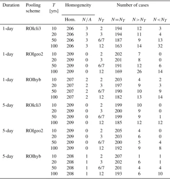
Table 8 summarizes the size of pooling groups when the three selected pooling schemes are applied to estimate the T-year growth factors of 1-day and 5-day precipitation max-ima. It is obvious that the majority of the pooling groups are homogeneous according to the Lu and Stedinger test of regional homogeneity in the initial stage of their forming, corresponding to the target size NT given by the 5T rule (column “N=NT” in Table 8). Provided that the pooling group is heterogeneous forNT, the procedure of successively adding similar sites to the pooling group (or removing dis-similar sites if necessary) mostly results in a homogeneous stage. Note that at the end of a pooling procedure, no het-erogeneous pooling groups appear. This fact stems from the way the pooling groups are constructed (Sect. 3.1). In the worst case, the pooling procedure ends up with a single-site pooling group; this is observed altogether in 6 cases related to 5 different stations. The reason the pooling procedure fails in these specific cases can be generalised as follows: For any of these 5 stations, the sites that show a considerable degree of similarity with the target site in terms of site attributes (in the attribute space) appear highly dissimilar in the site statistics. In other words, once a small heterogeneous pooling group is constructed, its degree of heterogeneity cannot be consider-ably reduced either by assigning the next closest sites to this pooling group or by gradually removing sites from it, since the core of the pooling group (the target site and the next few closest sites) still remains heterogeneous.

A further remarkable feature of Table 8 is that precipita-tion maxima of longer duraprecipita-tions show higher degree of ho-mogeneity compared to those of 1-day duration. This is un-derpinned by the fact that for the 5-day precipitation amounts the regional homogeneity is reached more often for the target size of the pooling groupsNT.

Generally, inter-comparison of the ROI pooling meth-ods suggests that the hybrid pooling schemes including also climatological characteristics may surpass the ROI method based on geographical distance for multi-day precipita-tion extremes, the spatial variability of which is less af-fected by random (sampling) variations and more closely linked to some regional patterns in central Europe related

Table 7. Average root mean square error (RMSE) of growth fac-tors of annual maxima of 1-day and 5-day precipitation amounts

for return periodT [years], expressed in %. The smallest values of

RMSE are marked in bold, separately for both durations. ROIhyb denotes the hybrid ROI pooling scheme ROIhybC-geo0.80.

1-day precipitation amounts 5-day precipitation amounts

T ROI ROI ROI

At-site ROI ROI ROI At-site

[yrs] cli3 geo2 hyb cli3 geo2 hyb

10 3.300 3.080 3.083 3.597 3.103 2.991 2.935 3.529

20 5.609 5.153 5.207 6.598 5.319 4.997 4.884 6.537

50 8.481 7.929 8.112 11.690 8.296 7.404 7.402 11.690

100 10.713 9.820 9.983 16.248 10.479 9.109 9.084 16.329

Fig. 6. Root mean square error (RMSE) of growth factors

corre-sponding to return periodsT=10, 20, 50 and 100 years for annual

maxima of 1-day and 5-day precipitation amounts in a compari-son of the performance of three selected pooling schemes (ROIcli3, ROIgeo2 and ROIhyb = ROIhybC-geo0.80, see Sect. 4.2) with the at-site frequency model.

to atmospheric circulation and orographic features. The re-gional differences in distributions of the multi-day extremes reflect, for example, the varied influences of cyclones of Mediterranean origin (which often produce heavy multi-day precipitation) between the eastern and western parts of the Czech Republic (e.g. Kysel´y and Picek, 2007b). For 1-day precipitation extremes, which are mostly related to convective phenomena in the warm season (88% of annual maxima of 1-day amounts occur in April–September), the ROI method based on geographical characteristics is clearly superior to all other pooling schemes.

5 Discussion and conclusions

Table 8.Summary statistics of pooling groups constructed accord-ing to three selected poolaccord-ing schemes (ROIcli3, ROIgeo2 and ROI-hyb = ROIROI-hybC-geo0.80, see Sect. 4.2) and for two durations of precipitation (1-day and 5-day). “Hom.” denotes number of ho-mogeneous pooling groups; “N/A” labels number of cases when re-gional heterogeneity/homogeneity cannot be defined, i.e. in the case

of single-site pooling groups.N (NT)yields the actual (target) size

of pooling groups.

Duration Pooling T Homogeneity Number of cases scheme [yrs]

Hom. N/A NT N=NT N >NT N <NT

1-day ROIcli3 10 206 3 2 194 12 3

20 206 3 3 194 11 4

50 206 3 6/7 187 9 13

100 206 3 12 163 14 32

1-day ROIgeo2 10 209 0 2 202 7 0

20 209 0 3 201 8 0

50 209 0 6/7 191 12 6

100 209 0 12 169 26 14

1-day ROIhyb 10 207 2 2 203 4 2

20 207 2 3 197 9 3

50 207 2 6/7 190 10 9

100 207 2 12 182 13 14

5-day ROIcli3 10 209 0 2 199 10 0

20 209 0 3 200 9 0

50 209 0 6/7 199 9 1

100 209 0 12 185 12 12

5-day ROIgeo2 10 209 0 2 205 4 0

20 209 0 3 203 6 0

50 209 0 6/7 200 5 4

100 209 0 12 192 9 8

5-day ROIhyb 10 208 1 2 207 1 1

20 208 1 3 202 6 1

50 208 1 6/7 201 4 4

100 208 1 12 193 6 10

methodology for estimatingT-year growth factors (i.e. the T-year values of the cumulative distribution function of di-mensionless data) of annual maxima of 1-day and 5-day pre-cipitation amounts by means of simulation experiments. The regional homogeneity test of Lu and Stedinger (1992) is in-corporated in order to avoid subjective decisions concern-ing the parameters involved in the ROI methodology and to avoid forming heterogeneous pooling groups for the estima-tion. The target number of sites in a pooling group is cho-sen according to the 5T rule (Jakob et al., 1999), i.e. a rule of thumb for the minimum number of sites within a pooling group needed for reliable estimation of aT-year quantile (or growth factor). Consequently, the size of the pooling groups varies with the return period of the growth factor to be esti-mated.

The first part of the sensitivity analysis, which examined the consequences of the changes made to the site attribute sets of the pooling schemes (while neglecting the relative weights), confirmed a simple principle “the more attributes included – the better performance” in the case of clima-tological site characteristics (used in the ROIcli models). On the other hand, in the case of geographical site char-acteristics (ROIgeo models), the pooling scheme ROIgeo2

based on geographical distance was found superior com-pared to ROIgeo3 that makes use of all three geographi-cal co-ordinates (i.e. latitude, longitude and altitude). In general, both alternatives to the ROIgeo models have their pros and cons. The main drawback of the ROIgeo3 pooling scheme is the tendency to pool sites from considerable dis-tances away from the target site, while the disadvantage of the ROIgeo2 pooling scheme is that it pools sites regardless of their altitudinal zonality. In the light of the dense pre-cipitation dataset available, however, the drawbacks of the ROIgeo2 model are less pronounced. Therefore, ROIgeo2 always outperforms the ROIgeo3 pooling scheme in terms of RMSE of the estimated growth factors in the present appli-cation.

The simulation experiments investigated also the effect of changes made to the “true” frequency model, which was used as a common platform for comparison of the examined pooling schemes in the Monte Carlo simulation. The results show that the relative performance of the selected pooling schemes (ROIgeo2, ROIgeo3 and ROIcli3) does not depend on changes made to the reference frequency model: the most (least) acceptable spread statistics appear in the case of the ROIgeo2 (ROIcli3) pooling scheme.

The second part of the sensitivity analysis focused on rea-sonable combinations of the geographical and climatologi-cal site attributes into hybrid pooling schemes by assigning different weights to the selected site attributes. The exten-sive simulation procedure showed that the actual proximity of sites is the most important factor in determining their sim-ilarity for the frequency analysis of precipitation extremes. However, there is a difference between the hybrid models for the two durations: while in the case of 1-day precipita-tion amounts there is no pooling scheme making use of a combination of climatological and geographical site charac-teristics that would outperform the pooling scheme based on the distance between sites (ROIgeo2), further climatological site characteristics do enhance the performance of the hybrid pooling schemes for multi-day amounts. This reflects the fact that multi-day extremes are more strongly linked to basic cli-matological characteristics of precipitation regimes than are 1-day extremes.

The comparison of the ROI pooling schemes with the at-site approach shows that the local estimates are not satis-factory when one is interested in estimating quantiles with longer return periods (T_≥10 years). The benefits of the pooling approaches over single-site analysis become obvious with increasingT.

Although the ROI approach, in general, allows for estimat-ing quantiles of extreme precipitation at ungauged sites, this paper was not aimed at addressing this issue. Even if we sup-pose that the climatological site characteristics at locations with no direct meteorological observations can be obtained using mapping techniques, the estimation of quantiles of ex-treme precipitation at ungauged sites raises questions as to estimating the index storm. That requires a more elaborate approach (e.g. Caporali et al., 2008; Brath et al., 2003) and is therefore beyond the scope of the current study.

Since the spatial resolution of the examined precipitation datasets (the density of sites corresponds to 1 station per an area of 19.4×19.4 km) is comparable to the resolution of most current regional climate model simulations over Eu-rope (about 25 km, see e.g. http://ensembles-eu.metoffice. com/results.html), the present findings may have implica-tions for pooling schemes applicable to estimating high quan-tiles of daily precipitation (and constructing their possible scenarios) in climate change simulations. It is often neces-sary to “smooth” the estimated distributions and/or quantiles of precipitation amounts (e.g. Semmler and Jacob, 2004) in order to reduce large spatial variability that is related to ran-dom fluctuations, and the ROI approach (with the geographi-cal distance in the dissimilarity matrix) appears to be a useful methodology that may easily and naturally be transferred to the context of climate model outputs. With increasing reso-lution of climate model simulations (and more data available for the estimation), the issue of how to efficiently reduce ran-dom sampling variability becomes more appealing.

Appendix A

Test of regional homogeneity by Lu and Stedinger

The test of regional homogeneity by Lu and Ste-dinger (1992), known as theX10 test, is based on the sam-pling variance of the 10-year growth factor of precipitation xT(T₌10)≡x10in a homogeneous region or pooling group. It is assumed that the precipitation extremes follow the gen-eralized extreme value (GEV) distribution (e.g. Coles, 2001). According to Fill and Stedinger (1995), the 10-year growth factor of precipitation at the i-th site x_(i)10 is estimated by means of L-moments as follows:

x_(i)10₌

 



1+₁₋t(i)₂−k

1−(−Ŵ(ln01₊.9k))k

if k₆₌0 1+2.4139t(i) if k₌0

(A1)

wheret(i)is the sample L-Cv (Eq. 5 in Sect. 3.2) at the i-th site, and i-the shape parameterkis estimated using the ap-proximation of Hosking et al. (1985):

k_≈7.8590c₊2.9554c2 (A2)

where c₌ 2

3+t3−

log2

log3 (A3)

andt3 is the sample L-skewness (Eq. 6 in Sect. 3.2). The

heterogeneity measure of theX10 test is then

χ_R2₌ N

X

i=1

x_(i)10₋x_R102

varx_(i)10 (A4)

whereN is the total number of sites in the region or pooling group,

x_R10₌ N

X

i₌1

nix10(i)

, _N

X

i₌1

ni (A5)

is the weighted regional average of x10_(i) (with the weights proportional to the record length ni), and varx_(i)10 is the asymptotic variance ofx_(i)10. The asymptotic variance is usu-ally determined by means of simulations, but Lu and Ste-dinger (1992) provide tables and correction factors (in case of short records) forvarx_(i)10.

The test statisticχ_R2 has an approximate chi-square distri-bution withN-1 degrees of freedom. Ifχ_R2<χ₀2_.95,N−1, the null hypothesis is not rejected at the 0.05 level and the pool-ing group may be considered homogeneous. In the opposite case, one rejects the null hypothesis and the pooling group is considered heterogeneous (Lu and Stedinger, 1992).

Acknowledgements. The study was supported by the young scientists’ research project B300420801 of the Grant Agency of the Academy of Sciences of the Czech Republic. Thanks are due to two anonymous reviewers and P. Allamano for comments on

the original manuscript; P.Stˇ ˇep´anek, Czech Hydrometeorological

Institute, for preparing the precipitation datasets; and O. Hal´asov´a, Czech Hydrometeorological Institute, for drawing Fig. 1.

Edited by: P. Molnar

References

Adamowski, K.: Regional analysis of annual maximum and partial duration flood data by nonparametric and L-moment methods, J. Hydrol., 229(3–4), 219–231, 2000.

Alila, Y.: A hierarchical approach for the regionalization of precip-itation annual maxima in Canada, J. Geophys. Res., 104(D24), 31645–31656, 1999.

Boni, G., Parodi, A., and Rudari, R.: Extreme rainfall events: Learning from raingauge time series, J. Hydrol., 327(3–4), 304– 314, 2006.

Brath, A., Castellarin, A., and Montanari, A.: Assessing the reliability of regional depth-duration-frequency equations for gaged and ungaged sites, Water Resour. Res., 39(12), 1367, doi:10.1029/2003WR002399, 2003.

Burn, D. H.: An appraisal of the “region of influence” approach to flood frequency analysis, Hydrolog. Sci. J., 35(2), 149–165, 1990a.

Burn, D. H.: Catchment similarity for regional flood frequency analysis using seasonality measures, J. Hydrol., 202(1–4), 212– 230, 1997.

Caporali, E., Cavigli, E., and Petrucci, A.: The index rainfall in the regional frequency analysis of extreme events in Tuscany (Italy), Environmetrics, 19, 7, 714–727, 2008.

Castellarin, A., Burn, D. H., and Brath, A.: Assessing the effec-tiveness of hydrological similarity measures for flood frequency analysis, J. Hydrol., 241(3–4), 270–287, 2001.

Chen, Y. D., Huang, G., Shao, Q., and Xu, C.-Y.: Regional analysis of low-flow using L-moments for Dongjiang basin, South China, Water Resour. Res., 51(6), 1051–1064, 2006.

Chowdhury, J. U., Stedinger, J. R., and Lu, L.-H.: Goodness-of-fit tests for regional generalized extreme value flood distribution, Water Resour. Res., 27(7), 1765–1776, 1991.

Clausen, B. and Pearson, C. P.: Regional frequency analysis of an-nual maximum streamflow drought, J. Hydrol., 173(1–4), 111– 130, 1995.

Coles, S.: An introduction to statistical modeling of extreme values, Springer-Verlag, London, 2001.

Cunderlik, J. M. and Burn, D. H.: Analysis of the linkage between rain and flood regime and its application to regional flood fre-quency estimation, J. Hydrol., 261(1–4), 115–131, 2002. Cunnane, C.: Methods and merits of regional flood frequency

anal-ysis, J. Hydrol., 100(1–3), 269–290, 1988.

Dalrymple, T.: Flood frequency analyses, Water Supply Paper 1543-A, US Geological Survey, Reston, USA, 1960.

Di Baldassarre, G., Castellarin, A., and Brath, A.: Relationships between statistics of rainfall extremes and mean annual precip-itation: an application for design-storm estimation in northern central Italy, Hydrol. Earth Syst. Sci., 10, 589–601, 2006, http://www.hydrol-earth-syst-sci.net/10/589/2006/.

Fill, H. D. and Stedinger, J. R.: Homogeneity tests based upon Gumbel distribution and a critical appraisal of Dalrymple test, J. Hydrol., 166(1–2), 81–105, 1995.

Fowler, H. J. and Ekstr¨om, M.: Multi-model ensemble estimates of climate change impacts on UK seasonal rainfall extremes, Int. J. Climatol., 29, 385–416, 2009.

Fowler, H. J. and Kilsby, C. G.: A regional frequency analysis of United Kingdom extreme rainfall from 1961 to 2000, Int. J. Cli-matol., 23, 1313–1334, 2003.

Ga´al, L. and Kysel´y, J.: Regional frequency analysis of heavy pre-cipitation in the Czech Republic by improved region-of-influence method, Hydrol. Earth Syst. Sci. Discuss., 6, 273–317, 2009, http://www.hydrol-earth-syst-sci-discuss.net/6/273/2009/. Ga´al, L., Kysel´y, J., and Szolgay, J.: Region-of-influence approach

to a frequency analysis of heavy precipitation in Slovakia, Hy-drol. Earth Syst. Sci., 12, 825–839, 2008a,

http://www.hydrol-earth-syst-sci.net/12/825/2008/.

Ga´al, L., Szolgay, J., and Lapin, M.: Regional frequency analysis of heavy precipitation totals in the High Tatras region in Slo-vakia, Contributions to Geophysics and Geodesy, 38(3), 327– 355, 2008b

Gabriele, S. and Arnell, N.: A hierarchical approach to regional flood frequency analysis, Water Resour. Res., 27(6), 1281–1289, 1991.

Gellens, D.: Combining regional approach and data extension pro-cedure for assessing of extreme precipitation in Belgium, J. Hy-drol., 268(1–4), 113–126, 2002.

GREHYS (Groupe de recherche en hydrologie statistique): Presen-tation and review of some methods for regional flood frequency analysis, J. Hydrol., 186(1–4), 63–84, 1996a.

GREHYS (Groupe de recherche en hydrologie statistique): Inter-comparison of regional flood frequency procedures for Canadian rivers, J. Hydrol., 186(1–4), 85–103, 1996b.

Holmes, M. G. R., Young, A. R., Gustard, A., and Grew, R.: A region of influence approach to predicting flow duration curves within ungauged catchments, Hydrol. Earth Syst. Sci., 6, 721– 731, 2002,

http://www.hydrol-earth-syst-sci.net/6/721/2002/.

Hosking, J. R. M.: L-moments: analysis and estimation of distri-butions using linear combinations of order statistics, J. Roy. Stat. Soc. B Met., 52(1), 105–124, 1990.

Hosking, J. R. M. and Wallis, J. R.: Some statistics useful in re-gional frequency analysis, Water Resour. Res., 29, 271–281, 1993.

Hosking, J. R. M. and Wallis, J. R.: Regional frequency analysis: an approach based on L-moments, Cambridge University Press, Cambridge, 1997.

Hosking, J. R. M., Wallis, J. R., and Wood, E. F.: Estimation of the generalized extreme-value distribution by the method of probability-weighted moments, Technometrics, 27, 251–261, 1985.

Jakob, D., Reed, D. W., and Robson, A. J.: Selecting a pooling-group, in: Flood Estimation Handbook, Vol. 3, Institute of Hy-drology, Wallingford, UK, 1999.

Jingyi, Z. and Hall, M. J.: Regional flood frequency analysis for the Gan-Ming River basin in China, J. Hydrol., 296(1–4), 98–117, 2004.

Kharin, V. V. and Zwiers, F. W.: Estimating extremes in transient climate change simulations, J. Climate, 18, 1156–1173, 2005. Kjeldsen, T. R., Smithers, J. D., and Schulze, R. E.: Regional flood

frequency analysis in the KwaZulu-Natal province, South Africa, using the index-flood method, J. Hydrol., 255(1–4), 194–211, 2002.

Kohnov´a, S., Szolgay, J., Sol´ın, L., and Hlavcov´a, K.: Regional_ˇ

methods for prediction in ungauged basins, Key Publishing, Os-trava, 2006.

Kysel´y, J.: Trends in heavy precipitation in the Czech

Re-public over 1961–2005, Int. J. Climatol., 2912, 1745–1758, doi:10.1002/joc.1784, 2009.

Kysel´y, J. and Picek, J.: Regional growth curves and improved de-sign value estimates of extreme precipitation events in the Czech Republic, Climate Res., 33, 243–255, 2007a.

Kysel´y, J. and Picek, J.: Probability estimates of heavy precipitation events in a flood-prone central-European region with enhanced influence of Mediterranean cyclones, Adv. Geosci., 12, 43–50, 2007b,

http://www.adv-geosci.net/12/43/2007/.

Lettenmaier, D. P., Wallis, J. R., and Wood, E. F.: Effect of regional heterogeneity on flood frequency estimation, Water Resour. Res., 23(2), 313–323, 1987.

Lu, L.-H. and Stedinger, J. R.: Sampling variance of normalized GEV/PWM quantile estimators and a regional homogeneity test, J. Hydrol., 138(1–2), 223–245, 1992.