Regional frequency analysis of heavy precipitation in the Czech Republic by improved region-of-influence method

(1)

HESSD

6, 273–317, 2009

ROI precipitation frequency analysis in

the Czech Republic

L. Ga ´al and J. Kysel´y

Title Page

Abstract Introduction

Conclusions References

Tables Figures

◭ ◮

Back Close

Full Screen / Esc

Printer-friendly Version

Interactive Discussion Hydrol. Earth Syst. Sci. Discuss., 6, 273–317, 2009

www.hydrol-earth-syst-sci-discuss.net/6/273/2009/ © Author(s) 2009. This work is distributed under the Creative Commons Attribution 3.0 License.

Hydrology and Earth System Sciences Discussions

Papers published inHydrology and Earth System Sciences Discussionsare under open-access review for the journalHydrology and Earth System Sciences

Regional frequency analysis of heavy

precipitation in the Czech Republic by

improved region-of-influence method

L. Ga ´al1,2and J. Kysel ´y1

1

Institute of Atmospheric Physics, Academy of Sciences of the Czech Republic, Boˇcn´ıII 1401, 141 31 Prague 4, Czech Republic

2

Department of Land and Water Resources Management, Faculty of Civil Engineering, Slovak University of Technology, Radlinsk ´eho 11, 813 68 Bratislava, Slovakia

Received: 16 December 2008 – Accepted: 18 December 2008 – Published: 14 January 2009 Correspondence to: L. Ga ´al ([email protected])

Published by Copernicus Publications on behalf of the European Geosciences Union.

(2)

HESSD

6, 273–317, 2009

Title Page

Tables Figures

◭ ◮

Back Close

Full Screen / Esc

Interactive Discussion Abstract

The region-of-influence (ROI) approach is implemented for modelling the probabilities of heavy 1-day and 5-day precipitation amounts in the Czech Republic. Compared to the previous study for Slovakia (Ga ´al et al., 2008), an improved ROI methodology that makes use of a regional homogeneity test for assigning sites to pooling groups,

5

is applied. Two basically different approaches to forming the pooling groups in which groups of sites are gradually built up and cut down, respectively, are combined. A sen-sitivity analysis, which examines the performance of the ROI models after changing the set of input site attributes that serve for determining the sites’ similarity, is carried out. Finally, several frequency models that include the ROI pooling schemes, a

conven-10

tional model based on fixed regions, and an at-site analysis are compared by means of Monte Carlo simulations. We conclude that, regardless of the duration of precipitation, the ROI pooling scheme based on the actual proximity of sites (latitude and longitude) outperforms the other frequency models in terms of the root mean square error of the growth curves.

15

1 Introduction

Frequency analysis, which aims at estimating recurrence intervals of heavy hydro-climatological phenomena, is a specific field of applied statistics, which has been in-tensively developed over recent decades. Frequency analysis usually benefits from a regional approach, which is applicable if the regional homogeneity criterion is met; that

20

is, the sites that form a given region share the same distribution function of the exam-ined variable apart from a site-specific scaling factor called the index value (Dalrymple, 1960). Di_fferent aspects of the regional approach to frequency analysis have been examined in connection with heavy precipitation (e.g. Gellens, 2002; Sveinsson et al., 2002; Fowler and Kilsby, 2003; Boni et al., 2006; Wallis et al., 2007), floods (e.g. Burn,

25

(3)

HESSD

6, 273–317, 2009

Title Page

Tables Figures

◭ ◮

Back Close

Full Screen / Esc

Interactive Discussion and Hall, 2004; Sol´_ın, 2008), droughts (e.g. Clausen and Pearson, 1999; Chen et al.,

2006), extreme sea levels (e.g. van Gelder et al., 2000) and wind speeds (e.g. Sotillo et al., 2006; Modarres, 2008).

The superiority of regional frequency models over the conventional at-site approach (which only utilizes data from the site of interest itself) stems not only from the reduced

5

uncertainty of the estimated high quantiles at the right tails of the distributions (e.g. Lettenmaier et al., 1987; Cunnane, 1988; Stedinger et al., 1993), but also from the fact that the regional methods allow for the estimation of design values at ungauged sites (e.g. GREHYS 1996a, b; Kohnov ´a et al., 2006b).

In the traditional approach to regional frequency analysis, the regions are kept fixed;

10

that is, when changing the focus from one site to another within a given region, the information source for the regional transfer remains unchanged (e.g. Hosking and Wal-lis, 1997). An alternative to regional frequency estimation, the region-of-influence ap-proach (ROI; Burn, 1990a, b), introduced a basically different concept: the idea of focused pooling. Its main feature is the uniqueness of the “regions” (more precisely,

15

the pooling groups – Reed et al., 1999b): each site under study has its own group of adequately similar sites that form the basis for the transfer of information on extremes to the site of interest. The idea of focused pooling has been adopted in studies of flood flows (e.g. Zrinji and Burn, 1994, 1996; Castellarin et al., 2001; Cunderlik and Burn, 2002; Holmes et al., 2002; Shu and Burn, 2004) and precipitation extremes

(Schae-20

fer, 1990; Alila, 1999; Di Baldassare et al., 2006), as well as in complex nationwide projects devoted to the frequency analysis of hydro-climatological extremes (Reed et al., 1999a; Thompson, 2002).

In an analysis of extreme precipitation amounts in Slovakia, Ga ´al et al. (2008) adopted an original concept of the ROI approach (Burn, 1990b), which, however, had

25

been subjected to criticism due to the need to choose a relatively large number of parameters according to subjective considerations (e.g. Hosking and Wallis, 1997). Zrinji and Burn (1994) revisited the ROI methodology: instead of subjectively selected threshold values, a built-in regional homogeneity test was used for assigning sites to a

(4)

HESSD

6, 273–317, 2009

Title Page

Tables Figures

◭ ◮

Back Close

Full Screen / Esc

Interactive Discussion given pooling group. They employedχ_R2 statistics (Chowdhury et al., 1991) for testing

the regional homogeneity of the proposed pooling groups. Later, Zrinji and Burn (1996) extended the ROI methodology by a hierarchical feature (Gabriele and Arnell, 1991), which implemented different alternatives to the homogeneity test of Hosking and Wallis (1993). Castellarin et al. (2001) applied the hierarchical pooling methodology of Zrinji

5

and Burn (1996) for a flood frequency analysis in northern central Italy.

In this study we modify the pooling methodology of Castellarin et al. (2001), carry out a sensitivity analysis by examining the performance of the ROI models after chang-ing the set of input site attributes that serve for determinchang-ing the sites’ similarity, and compare the improved ROI model with other frequency models by means of simulation

10

experiments. The methods are applied to modelling probabilities of extreme one-day and multi-day precipitation amounts in the Czech Republic (central Europe).

2 Data

2.1 Precipitation data

Daily precipitation totals measured at 209 stations mostly operated by the Czech

Hy-15

drometeorological Institute (CHMI) were used as the input dataset (Fig. 1). The alti-tudes of the stations range from 150 to 1490 m a.s.l., and the observations at most sites span the period from 1961 to 2005. Three main criteria were applied when selecting the stations and forming the dataset:

– the stations approximately evenly cover the area of the Czech Republic;

20

– there were no significant station moves during 1961–2005 (all sites where any location changes exceeded 50 m in altitude were excluded from the analysis), and no other sources of inhomogeneities were reported;

– the daily series of precipitation records are uninterrupted (except for the sites discussed below).

(5)

HESSD

6, 273–317, 2009

Title Page

Tables Figures

◭ ◮

Back Close

Full Screen / Esc

Interactive Discussion The data underwent standard quality checking for gross errors (cf. Coufal et al., 1992).

A large majority of the station records cover the whole period of 1961–2005; 36 out of the 209 stations have daily data over shorter subperiods of at least 31 consecutive years (mostly between 38 and 43 years; the stations started to operate after 1961 or closed before 2005) and/or minor parts of the records had to be omitted owing to the

5

stations’ relocations.

The dataset is superior to the one employed in Kysel´y and Picek (2007a), especially since it involves a much larger number of sites with complete daily records, more evenly covers the area of the Czech Republic, extends to the very recent past (December 2005), and a few errors in the original dataset were corrected (a missing month was

10

identified in the records of 3 stations, and the data were supplemented).

At 45 stations, minor gaps in the daily records occurred (a total of up to 1 month over 45 years at 32 sites and not exceeding 3 months at any of the 45 sites). We decided to preserve these stations in the analysis because of their locations in areas that are insufficiently covered by rain-gauges with complete records. The missing daily

15

data were estimated using measurements at 2 to 5 nearest locations available in the climatological database of the CHMI; the methodology is described in Kysel´y (2008). (Note that the mean distance to the nearest measuring site was only 15.4 km for the locations where the missing data were estimated, and the percentage of the missing daily records in the entire dataset was only 0.05%.) All other station records with more

20

than 3 months of missing values were excluded from the analysis.

The basic features of the precipitation climate of the Czech Republic, with a focus on extremes, may be found in Kysel´y and Picek (2007a) and Kysel´y (2008).

Samples of the annual maxima of 1-day and 5-day precipitation amounts were drawn from each station record and are further examined.

25

2.2 Alternatives of site attributes

The ROI approach as one of the methods of focused pooling techniques is aimed at finding groups of sites that share similar statistical properties of the observed

(6)

HESSD

6, 273–317, 2009

Title Page

Tables Figures

◭ ◮

Back Close

Full Screen / Esc

Interactive Discussion climatological extremes. It is assumed that the frequency distribution of the extremes at

a given site is closely related to its climatological, hydrological, geographical, geomor-phological, etc., attributes. Therefore, one of the basic issues of the pooling procedures is the selection of site attributes that are useful for explaining the observed behaviour of the extremes.

5

The similarity of sites in the pooling process is evaluated using two different sets of site attributes in this study.

The first group of site attributes consists of general climatological characteristics (abbr. ROIcli) that describe a long-term precipitation regime. The following variables are considered to be the basic characteristics of the precipitation climate:

10

1. mean annual precipitation [mm],

2. mean ratio of the precipitation totals for the warm/cold seasons [–], and

3. mean annual number of dry days [–] (defined as days with a precipitation amount ≥0.1 mm).

The warm (cold) season is defined as April–September (October–March). The basic

15

idea of the choice of the characteristics of the precipitation climate is that the atmo-spheric mechanisms generating heavy precipitation are similar under similar climato-logical conditions, particularly when the small extent of the study area is taken into account.

Geographical site characteristics (abbr. ROIgeo) represent the second group of

at-20

tributes that are employed to define the sites’ proximity:

1. latitude [degrees],

2. longitude [degrees] and

3. elevation above sea level [m].

The geographical co-ordinates are chosen since the actual proximity of the sites may

25

(7)

HESSD

6, 273–317, 2009

Title Page

Tables Figures

◭ ◮

Back Close

Full Screen / Esc

Interactive Discussion

3 Methods

3.1 Description of the pooling scheme

Since the pooling scheme adopted herein originates from that described in the details in Ga ´al et al. (2008), we confine the description to the cornerstones of the procedure and accentuate the changes and improvements in the methodology.

5

The similarity of sites in the attribute space is evaluated by means of a weighted Euclidean distance metric:

Di j =

" _M X

m=1

Wm

X_mi −X_mj2

#12

, (1)

whereDi j is the weighted Euclidean distance between sitesi andj;Wm is the weight associated with them-th site attribute; X_mi is the value of the m-th attribute at site i;

10

andM is the number of attributes. Before determining the elementsDi j of the distance metric or dissimilarity matrixD, the attributes undergo normalization in order to remove any possible bias from the estimation due to different magnitudes. The weight W_m in Eq. (1) is used to express the relative importance of the site attributes. In the current analysis, we use unit weighting coefficients for all the attributes (W_m=1, m=1, ..., M),

15

because we did not find any reasons to prefer one site attribute over another.

It is important to point out the di_fference between two types of the site attributes, which are usually termed as characteristics and statistics. Site characteristics are quantities independent of whether or not daily measurements of precipitation are car-ried out at a given site. These include geographical co-ordinates, geomorphological

20

attributes and/or descriptors of the long-term (precipitation) climate. On the other hand, site statistics are the results of the statistical processing of the data observed at a given site. It is generally recommended (Hosking and Wallis, 1997; Castellarin et al., 2001) to use site characteristics in the process of the formation of the regions or pooling

(8)

HESSD

6, 273–317, 2009

Title Page

Tables Figures

◭ ◮

Back Close

Full Screen / Esc

Interactive Discussion groups, while one should take advantage of site statistics in the process of testing the

homogeneity of a proposed group of sites.

Pooling groups in the ROI approach are generally constructed using elements D_{i j}

arranged in ascending or descending order; however, there are basically two different ways as to how to accomplish this. The core idea of the first method lies in the gradual

5

building up of the pooling groups (termed as the “forward” approach herein). Starting with the target sitei, which represents a single-site pooling group at the very beginning of the process, the next closest site (i.e. the sitej with the next lowest value of Di j,

j=1, ..., N) is appended to the existing ROI in each turn, until a given condition for forming the ROI is met. The process of building up the ROI is terminated (i) at a given

10

point, which is defined as a function of the selected quantiles of the dissimilarity matrix D(Burn, 1990b) or (ii) when the measure of the regional homogeneity of the proposed group of sites reaches or exceeds an unacceptable level (Castellarin et al., 2001). A reversed “backward” procedure is adopted in the second method of pooling: in its initial stage, all the sites in the analysis are supposed to form a superregion, so step by step,

15

the most dissimilar sites are removed from the bulk of the sites until the remaining group of sites is homogeneous (Zrinji and Burn, 1994).

We implemented the regional homogeneity test proposed by Lu and Stedinger (1992) when forming the regions, for two reasons: (i) its application is computation-ally straightforward, and (ii) according to the comparative study of Fill and Stedinger

20

(1995), it is one of the most powerful homogeneity tests. A brief description of Lu and Stedinger’s homogeneity test, also called the X10 test, is given in the Appendix B.

We tested both the “forward” and “backward” approaches to forming homogeneous ROIs and decided to form the ROIs primarily by gradual building up (“forward”) and using a homogeneity test for finding the cutoffpoint for the inclusion of the sites. The

25

(9)

HESSD

6, 273–317, 2009

Title Page

Tables Figures

◭ ◮

Back Close

Full Screen / Esc

Interactive Discussion As mentioned above, the basic idea of the “forward” pooling procedure is an iterative

building up of the ROI for the site of interest. In each step of the iteration, the next similar site is added to the existing ROI, and the homogeneity of the proposed pooling group is tested. In the event the proposed ROI is homogeneous, the procedure goes on with the next loop; otherwise, the procedure is stopped, and the formation of the

5

given ROI is finished.

After a detailed scrutiny of the preliminary outcomes of the analysis, we found it useful to slightly modify this pooling procedure. In a number of cases, the heterogeneity had been reached relatively early, i.e. after a few (<4–6) iterations. Neither was the adoption of the idea suggested by Castellarin et al. (2001) helpful, to stop the iteration

10

procedure when the heterogeneity of the ROI is detected for the second time (instead of the first time). In both cases, the difficulty is that a relatively high number of pooling groups consists of a small number of sites and do not meet the “5T rule” (Jakob et al., 1999), which suggests that for a reliable estimation of a design value corresponding to the return period T, one needs 5 times T station-years of data. Considering the

15

fact that the average length of observations at the selected stations is∼44 years (see Sect. 2.1), it is desirable to have at least 10–11 sites included in a pooling group for a reliable estimation of the 100-year precipitation quantiles.

We modified the pooling procedure of Castellarin et al. (2001) as follows:

– At the very beginning, the ROI of the target site consists of 11 stations (i.e. it

20

comprises the site itself and the 10 closest sites), regardless of whether this initial pooling group is homogeneous or not.

– The iteration procedure of testing the homogeneity and adding the next closest site to the pooling group goes on until the first heterogeneous pooling group is found preceded by at least one homogeneous pooling group. In this case, the

25

last homogeneous stage defines the final composition of the pooling group for the site.

(10)

HESSD

6, 273–317, 2009

Title Page

Tables Figures

◭ ◮

Back Close

Full Screen / Esc

Interactive Discussion to the initial ROI, the program code returns to the initial stage with 11 sites and

starts looking for a homogeneous composition by removing the least similar sites from the pooling group. The first homogeneous stage then defines the final com-position of the pooling group for the site. In the worst case, when the building nor the removing procedure leads to a homogeneous stage, the ROI consists of

5

nothing but the target site (i.e. a “single-site pooling group”).

3.2 Frequency model of Hosking and Wallis

The classical regional analysis of Hosking and Wallis (1993, 1997) consists in delin-eating fixed regions that are homogeneous according to the statistical characteristics of the probability distributions of the extremes, i.e. the at-site distributions are identical

10

except for a site-specific scaling factor.

The delineation of homogeneous regions for 1-day and 5-day precipitation extremes in the Czech Republic has been updated and modified with respect to the original one presented in Kysel´y and Picek (2007a). The reason for revisiting the original results of the homogeneity tests was a new dataset of daily precipitation amounts, which consists

15

of 209 stations (compared to 78 in Kysel´y and Picek, 2007a), extends to a more recent past (2005), and altogether covers 9197 station-years (compared to the original 3120). The two largest regions of the original regionalization became heterogeneous when the new data were considered; they have been split into 3 and 2 smaller (homogeneous) areas. The new regionalization recognizes 9 regions (Fig. 1) that are homogeneous

20

according to the X10 test of Lu and Stedinger (1992) as well as the H1 test of Hosking and Wallis (1993) with respect to the statistical distributions of the annual maxima of the 1-day to 7-day precipitation amounts.

3.3 Estimation of growth curves and quantiles

For the construction of regional (pooled) growth curves and the estimation of the

pre-25

(11)

HESSD

6, 273–317, 2009

Title Page

Tables Figures

◭ ◮

Back Close

Full Screen / Esc

Interactive Discussion Appendix A). The GEV distribution is widely used for modelling hydro-climatological

extremes worldwide (e.g. Alila, 1999; Smithers and Schulze, 2001; Castellarin et al., 2001; Kharin and Zwiers, 2000), and frequency analyses of precipitation extremes have also confirmed its applicability in central Europe (the Czech Republic – Kysel´y and Picek, 2007a; Slovakia – Kohnov ´a et al., 2006a).

5

The growth curves and precipitation quantiles are estimated using the L-moment-based index storm procedure (Hosking and Wallis, 1997). In the initial step, dimen-sionless data are calculated by rescaling by the sample meanµj (index storm):

xj,k =

Xj,k

µj

, j =1, ..., N, k =1, ..., nj, (2) whereX_j,k (x_j,k) denotes the original (dimensionless, rescaled) data;N is the number

10

of sites; andn_j denotes the sample size of thej-th site.

The dimensionless values of xj,k at site j are then used to compute the sample L-momentsl₁(j),l₂(j), . . . and L-moment ratios:

t(j)

=l₂(j).l₁(j) (3)

and

15

t(_rj)=l_r(j).l₂(j), r =3, 4, ..., (4) wheret(j) is the sample L-coefficient of variation (L-CV) andt_r(j), r=3, 4, ... are the sample L-moments ratios at sitej (Hosking, 1990).

The pooled (regional) L-moment ratiost(i)R and t_r(i)R,r=3, 4, ...for the target sitei

are derived from the at-site sample L-moment ratios as their weighted averages:

20

t(i)R = N

P

j=1

Wi jt(j)

N

P

j=1

Wi j

, (5)

(12)

HESSD

6, 273–317, 2009

Title Page

Tables Figures

◭ ◮

Back Close

Full Screen / Esc

Interactive Discussion whereW_{i j} are the weights associated with the j-th site in the analysis. The

relation-ships analogous to Eq. (5) also hold true fort(_ri)R,r=3, 4, ....

From a mathematical point of view, the most important difference between the tradi-tional regionalization and the focused pooling consists in the way the weighting coe_ffi -cientsW_{i j}in Eq. (5) are defined. In the traditional regional analysis,W_{i j}are proportional

5

only to the record lengthn_j for all the sitesjwithin a given region:

Wi j =

n_j _∀j _∈R_i

0 ∀j /∈R_i , (6)

whereRi denotes the region to which the target sitei belongs. Equation (6) is in accor-dance with the concept of Hosking and Wallis (1997): sites with longer observations provide more information in the regionally averaged statistics. Note that the regional

10

weighting coefficients in Eq. (6) do not change when changing the focus from one site to another within a given region.

In the focused pooling, the length of observationsn_j is retained in the relationship for

W_{i j}; however, compared to Eq. (6), the reciprocal value of the distance metric element

Di j is introduced as an additional factor (Castellarin et al., 2001):

15

Wi j =

(

nj

.

D∗_{i j} ∀j ∈ROI_i

0 ∀j /∈ROI_i , (7)

where ROI_i stands for the region of influence of the sitei, and

D∗ i j =

D_{i j} ifD_{i j}6=0

Di j,min ifDi j=0

, (8)

whereD_{i j,}minis the lowest non-zero value of the distance metric between the target site

i and all the other sitesj (Castellarin et al., 2001). (The expression forD∗_{i j} in Eq. (8) is

20

(13)

HESSD

6, 273–317, 2009

Title Page

Tables Figures

◭ ◮

Back Close

Full Screen / Esc

D_{i j} as the pooled weighting factor is equivalent to assigning higher weights to sites that lie in the proximity of the target site in the attribute space: the smallerDi j for a given sitejis, the greater the amount of information it brings to the procedure for the growth curve estimation at sitei.

The regionally weighted (pooled) L-moment ratiost(i)R andt_r(i)R,r=3, 4, ...are then

5

used to estimate the parameters of the GEV distribution and the dimensionless cumu-lative distribution function (the growth curve). A quantile corresponding to the return periodT is calculated as a product of the dimensionlessT-year growth curve valuex_iT

and the index stormµ_i:

X_iT =µ_ixT_i . (9)

10

3.4 Framework for an inter-comparison of the frequency models

In this paper, ROI pooling schemes based on climatological and geographical site at-tributes (Sect. 2.2) are compared with other frequency models, which include (i) the conventional regionalization approach of Hosking and Wallis (1997; abbr. HWreg), and (ii) the at-site frequency analysis. The performance of the di_fferent frequency models

15

is assessed by means of Monte Carlo simulation procedures.

The essential issue of the Monte Carlo simulation is the way the unknown parent dis-tribution (the “true” disdis-tribution) of the extremes is estimated. We decided to estimate the “true” at-site distribution by adopting the region-of-influence approach in which the similarity of sites is determined according to the statistical properties of the at-site data

20

samples (abbr. ROIsta), as in Castellarin et al. (2001) and Ga ´al et al. (2008). Three site statistics were selected (cf. Burn, 1990b; Ga ´al et al., 2008):

1. the coefficient of variation: c_v=σ

µ, where µ(σ) is the sample mean (standard deviation);

2. Pearson’s 2nd skewness coefficient: P S=3 (µ−m)σ, wheremis the sample

me-25

dian (Weisstein, 2002);

(14)

HESSD

6, 273–317, 2009

Title Page Abstract Introduction Conclusions References Tables Figures ◭ ◮ ◭ ◮ Back Close

Full Screen / Esc

Interactive Discussion 3. the normalized 10-year precipitation quantile, estimated using the GEV

distribu-tion (x10y).

The selected statistics characterize the scale (c_v), shape (PS) and location (x10y) of the empirical distribution of the samples. A pooling scheme based on the site statistics is supposed to result in groups of sites that have a frequency distribution of extremes

5

similar to the target site.

In each loop of the Monte Carlo procedure, samples of the annual maxima that re-semble the real world (the actual number of sites, the length of the observations, and the spatial correlations between the sites) are simulated. At each site, the parent distri-bution is the GEV; its parameters correspond to the pooled L-moments according to the

10

ROIsta pooling scheme. Having simulated the at-site samples, the pooling schemes and frequency models described above are applied to estimate theT-year quantiles of the precipitation extremes, which are then compared with the “true” quantiles obtained by the ROIsta pooling scheme. The loops of the Monte Carlo simulations are repeated 5000 times.

15

The different frequency models are compared by means of the bias and the root mean square error (RMSE) statistics. For a given return periodT,

RMSET ₌ 1

N

X

i=1   1 M M X m=1 ˆ

x_{i ,m}T −xT_i x_iT

!2



1 2

(10)

and

BIAST=1

N

X

i=1

1

M

X

m=1

ˆ

x_{i ,m}T ₋x_iT x_iT

!

, (11)

20

(15)

HESSD

6, 273–317, 2009

Title Page

Tables Figures

◭ ◮

Back Close

Full Screen / Esc

Interactive Discussion The Monte Carlo simulation procedure and some related considerations are

de-scribed in more detail in Ga ´al et al. (2008, Sect. 4).

4 Results

4.1 Sensitivity analysis

A sensitivity analysis was performed in order to explore the role of different site

char-5

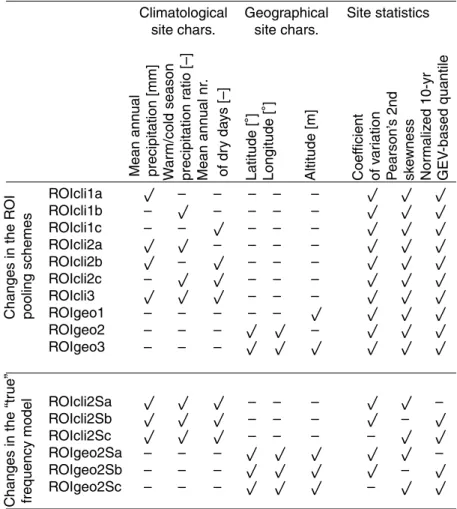
acteristics and site statistics entering the dissimilarity matrixD(Eq. 1) and to identify the optimum setting of the ROI pooling schemes. The basic ROI schemes were anal-ogous to those used in Ga ´al et al. (2008); the models were based on 3 climatological (geographical) site characteristics (Sect. 2.2), and labelled as ROIcli3 (ROIgeo3); both were connected with the model ROIsta based on 3 site statistics (ROIsta3) used for

10

the estimation of the “true” quantiles during the simulation procedures (Sect. 3.4). The sensitivity analysis examined the performance of the ROI models after removing one or two site attributes from the basic ROI pooling schemes (ROIcli3, ROIgeo3) or from the “true” frequency model (ROIsta3). The analysis was divided into two parts: (i) to ex-amine the effects of changes made to the basic ROI schemes, while keeping the “true”

15

model unchanged, and (ii) to examine the effects of changes in the “true” frequency model, while using the basic ROI schemes with 3 parameters. The different alterna-tives of the newly constructed ROI pooling schemes and the modified “true” frequency models are summarized in Table 1. Note that the number of alternatives to the ROIgeo models is reduced: While the ROIcli alternatives make use of all 6 possible

combi-20

nations of the 3 available climatological attributes into singles (labelled as ROIcli1a, b and c) or pairs (labelled as ROIcli2a, b and c), there are no reasons for using other simplified ROIgeo models than those based purely on elevation (ROIgeo1) or the pair of geographical co-ordinates (ROIgeo2). Furthermore, the modified “true” frequency models are based only on pairs of possible combinations of the site statistics defined

25

in Sect. 3.4 (labelled with the suffixes “2Sa”, “2Sb” and “2Sc”) since it is unreasonable

(16)

HESSD

6, 273–317, 2009

Title Page

Tables Figures

◭ ◮

Back Close

Full Screen / Esc

Interactive Discussion to construct “true” models based purely on one statistic. The sensitivity analysis was

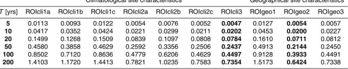
performed for both data sets of the 1-day and 5-day annual maxima.

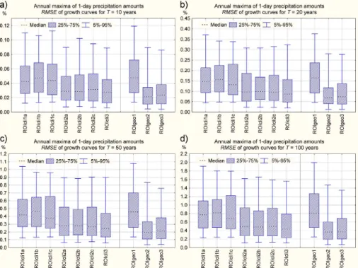
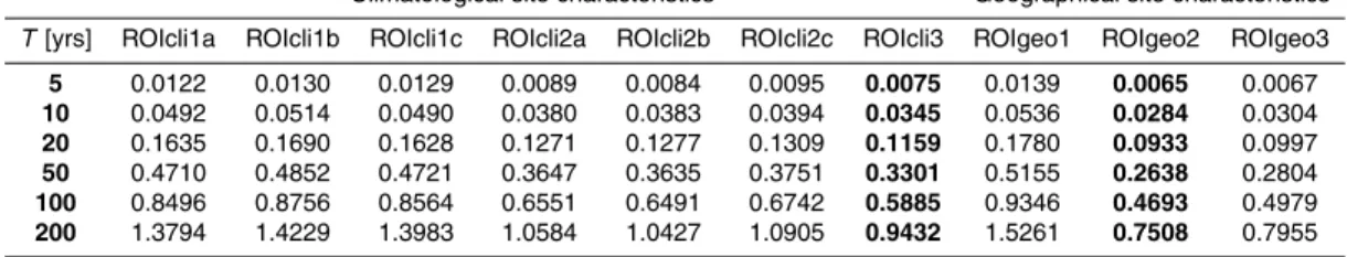
First, we focus on the consequences of the changes made to the basic pooling schemes ROIcli3 and ROIgeo3. The summary statistics of the models’ performance in terms of the average RMSE and the average bias for the quantiles of the estimated

5

distributions of the 1-day (5-day) maxima corresponding toT=5, 10, 20, 50, 100 and 200 years are given in Table 2 (Table 3); the box-and-whisker plots of the RMSE in Fig. 2 (Fig. 3) illustrate the spread statistics. In general, growth curves of the various models do not differ much in terms of the bias: that is why the box plots of the bias are not shown herein.

10

It is obvious that the ROI models based purely on a single site attribute show a very poor degree of performance: the average RMSE is approximately 50% higher (in some cases, especially for the 5-day duration, by ∼100% – Table 3) than for the best ROI models based on more than one site attribute. These results are in accordance with one’s expectation: the frequency behaviour of the precipitation extremes cannot be

ex-15

plained by a single climatological characteristic. The ROIcli2 models based on two site attributes clearly perform better; however, the best average and spread characteristics of the RMSE are obtained for the basic ROIcli3 model for both data sets (for 5-day du-rations, there are three models based on≥2 attributes with a comparable performance; the odd one is the ROIcli2b model, which suggests that the missing site characteristic

20

of the warm/cold season precipitation ratio (Sect. 2.2) plays an important role in the other ROIcli models).

While for the ROIcli models, more site attributes improve performance, a similar conclusion cannot be drawn for the ROIgeo pooling schemes: the ROIgeo2 model always outperforms the basic ROIgeo3 model (Tables 2–3, Figs. 2–3). Such behaviour

25

is accounted for by the role of the elevation in ROIgeo3: while in ROIgeo2, sites are pooled according to the geographical distance from the site of interest, ROIgeo3 gives preference to sites that are located in similar altitudes as the target one.

(17)

Olo-HESSD

6, 273–317, 2009

Title Page

Tables Figures

◭ ◮

Back Close

Full Screen / Esc

Interactive Discussion mouc, which are located not far from each other (40 km) but in different altitudes (750

and 225 m a.s.l., respectively). Pooling groups for the 1-day annual maxima at these stations according to both models are shown in Fig. 4, and some basic statistical char-acteristics of the composition of the pooling groups are summarized in Table 4.

Figure 4a (Fig. 4b) illustrates the pooling group for the ˇCerven ´a station according to

5

ROIgeo2 (ROIgeo3). There is a relatively clear pattern of the distribution of the sites belonging to the ROI around the target site in ROIgeo2 (Fig. 4a): the further apart they are located, the less weight is assigned to them, and the weights are obviously independent on the elevation. A larger spread of sites in a broader neighbourhood of the target station appears in ROIgeo3 (Fig. 4b): sites located at similar altitudes are

10

preferred over those in the very proximity of the target site, which is also underpinned by the fact that even sites from over 200 km are included in the ROI. Similar spatial patterns are observed for the Olomouc station (Figs. 4c–d) when comparing ROIgeo2 and ROIgeo3, although the di_fferences between the two pooling groups are not that large, mainly because many neighbouring stations are also located at similar altitudes.

15

Generally, when comparing the pooling groups in both models, the pooling groups of the ROIgeo3 model exhibit a greater average distance between the target site and the other sites within the ROI and a narrower elevation range (Table 4). Analogous findings hold true for the other pairs of stations, which are located not far from each other and at different altitudes.

20

The effects of the changes made to the “true” frequency model are summarized in Tables 5–6 and Figs. 5–6. Both the average values and spread statistics of the RMSE indicate that the best “true” model is the one based on all three statistical character-istics, regardless of the data set (1-day/5-day precipitation maxima) and the pooling scheme (ROIcli3/ROIgeo3). Such a conclusion is also underpinned by the spread

25

characteristics of the bias: the narrowest box-and-whisker plots are always related to the models based on the basic version of the “true” ROISsta3 model.

The performance of the modified “true” models with the suffixes “2Sa”, “2Sb” and “2Sc” allows for the ranking of the individual site statistics according to their

(18)

HESSD

6, 273–317, 2009

Title Page

Tables Figures

◭ ◮

Back Close

Full Screen / Esc

Interactive Discussion tance. The ROIcli2Sc/ROIgeo2Sc models show the worst statistical properties, which

suggests that the missing coefficient of variation plays the most important role among the selected site statistics in the “true” frequency models. On the other hand, the Pearson’s 2nd coefficient is the least important statistic, since when it is ignored, the ROIcli2Sb/ROIgeo2Sb models perform nearly as well as the best “true” model.

5

Similar Monte Carlo simulations (examining changes made to the “true” frequency model) were also carried out for the ROIgeo2 pooling scheme (not shown); the general features of its performance in the light of “true” frequency models based on diff er-ent input statistics are analogous to those for the basic ROIcli3 and ROIgeo3 pooling schemes.

10

4.2 Inter-comparison of the frequency models

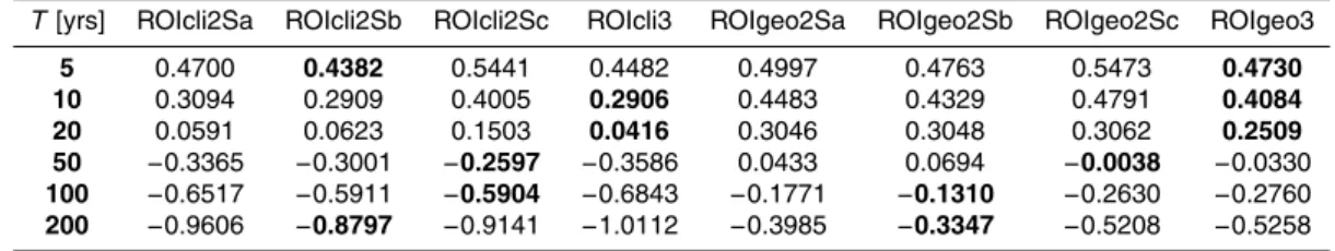
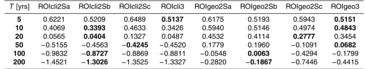
Tables 7–8 and Figs. 7–8 summarize the performance of the frequency models for 1-day and 5-1-day precipitation amounts, which correspond to different concepts: the two superior ROI models (based on three climatological and two geographical character-istics, ROIcli3 and ROIgeo2, respectively – Sect. 4.1), the Hosking-Wallis approach

15

based on fixed regions (HWreg – Sect. 3.2), and the at-site (local) estimates. The average values of the root mean square error in Tables 7–8 reveal that the at-site ap-proach, regardless of the duration, is clearly inferior, since the RMSE statistics of the local model are worse nearly by a magnitude compared to the other models. The poor performance of the at-site approach is explained by the enhanced effects of the

20

sampling fluctuations, which are reduced by the multi-site approach in the regional models/pooling schemes (cf. Hosking and Wallis, 1997; Ga ´al et al., 2008). That is why we focus on a comparison of the regional/pooling approaches hereafter.

The ROIgeo2 pooling scheme outperforms the other models in terms of the average RMSE for both durations (Tables 7–8). The spread statistics of the RMSE in Fig. 8

25

(19)

HESSD

6, 273–317, 2009

Title Page

Tables Figures

◭ ◮

Back Close

Full Screen / Esc

Interactive Discussion the return levels suggest that ROIgeo2 is superior for the 5-day maxima, too (the

per-centage of sites at which the RMSE is large is reduced more efficiently compared to the other models). Another disadvantage of the HWreg model is a slight tendency towards a negative bias for both 1-day and 5-day durations (Fig. 7).

The results suggest that the Hosking-Wallis regional analysis may compete with the

5

ROI method based on geographical characteristics only for multi-day precipitation ex-tremes, the spatial variability of which is less affected by random (sampling) variations and more closely linked to some regional patterns in central Europe, which are re-lated to atmospheric circulation and orographic features. The regional differences in the distributions of the multi-day extremes reflect, for example, the varied influences of

10

Mediterranean cyclones (which often produce heavy multi-day precipitation) between the eastern and western parts of the country (e.g. Kysel´y and Picek, 2007b). For one-day precipitation extremes, which are mostly related to convective phenomena in the warm season (88% of one-day maxima occurs in April-September), the ROI method based on geographical characteristics is clearly superior to all other frequency models,

15

including the Hosking-Wallis regional analysis.

On the other hand, it is worth noting that the Hosking-Wallis regional analysis out-performs the ROI model based on climatological characteristics for both durations of precipitation extremes, which contrasts with the results for Slovakia (Ga ´al et al., 2008). It is likely related to the choice of the climatological characteristics in Slovakia,

particu-20

larly the availability of the Lapin’s index of Mediterrenean influence (Ga ´al, 2005), which is closely linked to the occurrence of heavy precipitation (see also Sect. 5 below); no analogous index is available for the area of the Czech Republic. Another reason may be a different approach to the delineation of the homogeneous regions for the Hosking-Wallis analysis in the two countries, with 3 contiguous regions in Slovakia compared to

25

9 regions in the Czech Republic, which also take into account the altitudinal zonality, and therefore not all of them are contiguous.

(20)

HESSD

6, 273–317, 2009

Title Page

Tables Figures

◭ ◮

Back Close

Full Screen / Esc

5 Discussion and conclusions

The paper deals with the estimation of growth curves of the annual maxima of 1-day and 5-day precipitation amounts in the Czech Republic by improved region-of-influence (ROI) methodology. The improvements consist in the way the pooling groups are con-structed. The regional homogeneity test of Lu and Stedinger (1992) is incorporated

5

in order to avoid subjective decisions concerning the parameters involved in the ROI methodology, and to avoid forming heterogeneous pooling groups for the estimation. The remaining parameter in the improved ROI method, the “baseline” number of sites in a pooling group, is chosen according to the “5T rule” (Jakob et al, 1999), i.e. a rule of thumb for the minimum number of sites within a pooling group needed for a reliable

10

estimation of aT-year quantile (set to 100 years herein). The proposed ROI method-ology combines two different concepts of constructing the pooling groups described previously in hydrological studies (the “backward” approach of Zrinji and Burn, 1994, and the “forward” approach of Castellarin et al., 2001), and preserves some of their beneficial features:

15

1. Reasonably large numbers of sites in the pooling groups typical for a pooling scheme based on the strategy of gradual building up (Castellarin et al., 2001); too large pooling groups tend to be formed by the “backward” approach, which may smooth spatial details. For example, applying the ROIgeo3 scheme for the 1-day maxima in the present study, the average number of stations in the pooling

20

groups is 49.0, 49.3, and 70.5 according to the “forward” approach of Castellarin et al. (2001), our modified method, and the “backward” approach of Zrinji and Burn (1994), respectively.

2. Small numbers of the pooling groups with insufficient number of sites typical for a pooling scheme based on the strategy of cutting down (Zrinji and Burn, 1994).

25

(21)

HESSD

6, 273–317, 2009

Title Page

Tables Figures

◭ ◮

Back Close

Full Screen / Esc

Interactive Discussion the “forward” approach of Castellarin et al. (2001), our modified method, and the

“backward” approach of Zrinji and Burn (1994), respectively.

A sensitivity analysis, which examined the consequences of the changes made to the input attribute sets of the pooling schemes, confirmed a simple principle “the more in-put variables – the better performance” in the case of climatological site characteristics

5

(used in the ROIcli models) and site statistics (used in the ROIsta pooling scheme as the “true” frequency model in the simulation procedure). On the other hand, in the case of geographical site characteristics (used in the ROIgeo models), the pooling scheme based on two co-ordinates (latitude and longitude) was found superior compared to the one that makes use of all three co-ordinates (including altitude). In general, however,

10

both alternatives to the ROIgeo models have their own pros and cons. The main draw-back of the ROIgeo3 pooling scheme is the tendency to pool sites from considerable distances away from the target site, while the disadvantage of the ROIgeo2 pooling scheme is that it pools sites regardless of their altitudinal zonality. However, the draw-backs of the ROIgeo2 model are less pronounced; therefore, it always outperforms

15

the ROIgeo3 pooling scheme in terms of the RMSE of the estimated quantiles in the present application. An open question is whether some combination of the geographi-cal and climatologigeographi-cal characteristics would result in a model that outperforms the ROI schemes based on either geographical or climatological attributes, and whether there are other useful site attributes in addition to those examined; these issues go outside

20

the scope of the study and deserve further investigation.

The main finding concerning the inter-comparison of various regional frequency models is that the ROI pooling scheme based on the actual proximity of sites (latitude and longitude) outperforms the other models (including the Hosking-Wallis regional analysis), regardless of the duration of the precipitation extremes. Such a conclusion,

25

in general, is in good agreement with the findings of Ga ´al et al. (2008) who also showed the superiority of the pooling approach over the other frequency models, when analyz-ing the precipitation data in Slovakia. Nevertheless, they pointed out that different dura-tions need different ROI approaches: while the pooling scheme based on geographical

(22)

HESSD

6, 273–317, 2009

Title Page

Tables Figures

◭ ◮

Back Close

Full Screen / Esc

Interactive Discussion attributes is preferable for 1-day maxima, the ROI model based on climatological

at-tributes shows better statistical properties for 5-day durations. The difference between the main findings of the two studies may be related to the following causes:

– The more rugged terrain of Slovakia (the mountain range of the West Carpathians belt, including the High and Low Tatras, prolonged from west to east), which may

5

enhance the role of climatological characteristics in the identification of similar patterns of the precipitation extremes;

– A different suite of climatological characteristics used in the analysis for Slovakia, with Lapin’s index of Mediterranean influence (Ga ´al, 2005); no similar index of precipitation climate related to extremes is available for the Czech Republic;

10

– The poorer performance of the pooling schemes based on three geographical characteristics in Slovakia, which is likely due to the higher altitudinal variability of the selected sites in the country (a much larger percentage of higher-elevated sites at altitudes>1000 m a.s.l.);

– The denser network of the sites available in the Czech Republic (about one site

15

per 400 km2) compared to Slovakia (about one site per 900 km2), which tends to give preference to the similarity of sites based on geographical proximity rather than climatological characteristics.

One may argue that in the present study, pooling schemes based on climatological characteristics show a poorer performance due to failing to choose the right attributes

20

for the analysis. We used the same set of site characteristics (Sect. 2.2) that had constituted the basis for the identification of homogeneous regions in the traditional regionalization (Sect. 3.2; Kysel´y and Picek, 2007a), in order to preserve consistency. Furthermore, the selected climatological attributes are among the most appropriate descriptors of the precipitation climate. Therefore, it may be more reasonable to

ex-25

(23)

HESSD

6, 273–317, 2009

Title Page

Tables Figures

◭ ◮

Back Close

Full Screen / Esc

Interactive Discussion climatological characteristics. An objective method for identifying the proper weights

Wm for the site attributes in the dissimilarity matrix (Eq. 1) would have to be imple-mented for this purpose.

Appendix A

5

The generalized extreme value distribution

The cumulative distribution function of the generalized extreme value (GEV) distribution is

F(x;ξ, α, k)=



 

 

exp

−h1₋kx−_αξi−1/k

if k6=0 expn₋exph₋x−_αξio if k=0

, (A1)

whereξ, α and k is the location, scale and shape parameter, respectively (Hosking

10

and Wallis, 1997). The parameters satisfy _−∞<ξ<∞, α>0 and _−∞<k<∞. For an estimation of the parameters, we use the approximation of Hosking et al. (1985):

k≈7.8590c+2.9554c2, c= 2 3+t3

−log 2

log 3, (A2)

α= l2k 1−2−k

Γ(1+k), (A3)

and

15

ξ=l1−

α

k [1−Γ(1+k)], (A4)

wheret3is the sample L-skewness, l1 and l2 are the first two sample L-moments (cf.

Hosking and Wallis, 1997) andΓ(·) denotes the gamma function

Γ(x)=

Z_∞ 0

(24)

HESSD

6, 273–317, 2009

Title Page Abstract Introduction Conclusions References Tables Figures ◭ ◮ ◭ ◮ Back Close

Full Screen / Esc

Interactive Discussion Appendix B

Regional homogeneity test by Lu and Stedinger

The regional homogeneity test by Lu and Stedinger (1992), which is known as the X10 test, is based on the sampling variance of the dimensionless 10-year precipitationx10 5

in a homogeneous region. It is assumed that the precipitation extremes follow the GEV distribution (Eq. A1). According to Fill and Stedinger (1995), the 10-year quantile of the growth curve of precipitation at thei-th sitex(₁₀i) is estimated by means of L-moments as follows:

x₁₀(i) =







1+₁₋t(i)₂−k

1−(−ln 0.9) k Γ(1+k)

if k6=0 1+2.4139t(i) if k=0

. (B1)

10

wheret(i)is the sample L-Cv (Eq. 3 in Sect. 3.3) at thei-th site, and the shape param-eterk is estimated by Eq. (A2).

The heterogeneity measure of the X10 test is then

χ_R2 = N

X

i=1

x₁₀(i)−xR₁₀2

varx₁₀(i)

, (B2)

whereN is the total number of sites in the region,

15

x₁₀R = N

X

i=1

nix

(i) 10

, _N X

i=1

ni (B3)

is the weighted regional average of x₁₀(i) (with the weights proportional to the record lengthni), and varx

(i)

10 is the asymptotic variance of x (i)

(25)

HESSD

6, 273–317, 2009

Title Page

Tables Figures

◭ ◮

Back Close

Full Screen / Esc

Interactive Discussion usually determined by means of simulations; however, Lu and Stedinger (1992) provide

tables and small-sample correction factors for varx(₁₀i).

The test statisticχ_R2has an approximate chi-square distribution withN−1 degrees of freedom. Ifχ_R2<χ₀2_.₉₅_{, N}₋₁, the null hypothesis is not rejected at the 0.05 level and the region may be considered homogeneous. In the opposite case, one rejects the null

5

hypothesis and the region is considered heterogeneous (Lu and Stedinger, 1992).

Acknowledgements. The study was supported by the young-scientists’ research project B300420801 of the Grant Agency of the Academy of Sciences of the Czech Republic. Thanks are due to P. ˇSt ˇep ´anek, Czech Hydrometeorological Institute, for preparing the precipitation datasets; J. Picek, Technical University of Liberec, for providing the results of regional

homo-10

geneity tests for the Hosking-Wallis analysis; and O. Hal ´asov ´a, Czech Hydrometeorological Institute, for drawing Figs. 1 and 4.

References

Adamowski, K.: Regional analysis of annual maximum and partial duration flood data by non-parametric and L-moment methods, J. Hydrol., 229(3–4), 219–231, 2000.

15

Alila, Y.: A hierarchical approach for the regionalization of precipitation annual maxima in Canada, J. Geophys. Res., 104(D24), 31645–31656, 1999.

Boni, G., Parodi, A., and Rudari, R.: Extreme rainfall events: Learning from raingauge time series, J. Hydrol., 327(3–4), 304–314, 2006.

Burn, D. H.: An appraisal of the ‘region of influence’ approach to flood frequency analysis,

20

Hydrol. Sci. J., 35(2), 149–165, 1990a.

Burn, D. H.: Evaluation of regional flood frequency analysis with a region of influence approach, Water Resour. Res., 26(10), 2257–2265, 1990b.

Burn, D. H.: Catchment similarity for regional flood frequency analysis using seasonality mea-sures, J. Hydrol., 202(1–4), 212–230, 1997.

25

Castellarin, A., Burn, D. H., and Brath, A.: Assessing the effectiveness of hydrological similarity measures for flood frequency analysis, J. Hydrol., 241(3–4), 270–287, 2001.

Chen, Y. D., Huang, G., Shao, Q., and Xu, C.-Y.: Regional analysis of low-flow using L-moments for Dongjiang basin, South China, Water Resour. Res., 51(6), 1051–1064, 2006.

(26)

HESSD

6, 273–317, 2009

Title Page

Tables Figures

◭ ◮

Back Close

Full Screen / Esc

Chowdhury, J. U., Stedinger, J. R., and Lu, L.-H.: Goodness-of-fit tests for regional generalized extreme value flood distribution, Water Resour. Res., 27(7), 1765–1776, 1991.

Clausen, B. and Pearson, C. P.: Regional frequency analysis of annual maximum streamflow drought, J. Hydrol., 173(1–4), 111–130, 1995.

Coufal, L., Langov ´a, P., and M´ıkov ´a, T.: Meteorological data in the Czech Republic in the period

5

1961-1990. National Climatic Programme, Czech Hydrometeorological Institute, Prague, 160 pp., 1992 (in Czech).

Cunderlik, J. M. and Burn, D. H.: Analysis of the linkage between rain and flood regime and its application to regional flood frequency estimation, J. Hydrol., 261(1–4), 115–131, 2002. Cunnane, C.: Methods and merits of regional flood frequency analysis, J. Hydrol., 100(1–3),

10

269–290, 1988.

Dalrymple, T.: Flood frequency analyses, Water Supply Paper 1543-A., US Geological Survey, Reston, USA, 1960.

Di Baldassarre, G., Castellarin, A., and Brath, A.: Relationships between statistics of rainfall extremes and mean annual precipitation: an application for design-storm estimation in

north-15

ern central Italy, Hydrol. Earth Syst. Sci., 10, 589–601, 2006, http://www.hydrol-earth-syst-sci.net/10/589/2006/.

Fill, H. D. and Stedinger, J. R.: Homogeneity tests based upon Gumbel distribution and a critical appraisal of Dalrymple test, J. Hydrol., 166(1–2), 81–105, 1995.

Fowler, H. J. and Kilsby, C. G.: A regional frequency analysis of United Kingdom extreme rainfall

20

from 1961 to 2000, Int. J. Climatol., 23, 1313–1334, 2003.

Ga ´al, L., Kysel´y, J., and Szolgay, J.: Region-of-influence approach to a frequency analysis of heavy precipitation in Slovakia, Hydrol. Earth Syst. Sci., 12, 825–839, 2008,

http://www.hydrol-earth-syst-sci.net/12/825/2008/.

Ga ´al, L.: Introduction of Lapin’s indices into the cluster analysis of maximum k-day precipitation

25

totals in Slovakia, Meteorol. J., 8(2), 85–94, 2005.

Gabriele, S. and Arnell, N.: A hierarchical approach to regional flood frequency analysis, Water Resour. Res., 27(6), 1281–1289, 1991.

Gellens, D.: Combining regional approach and data extension procedure for assessing of ex-treme precipitation in Belgium, J. Hydrol., 268(1–4), 113–126, 2002.

30

GREHYS (Groupe de recherche en hydrologie statistique): Presentation and review of some methods for regional flood frequency analysis, J. Hydrol., 186(1–4), 63–84, 1996a.

(27)

HESSD

6, 273–317, 2009

Title Page

Tables Figures

◭ ◮

Back Close

Full Screen / Esc

frequency procedures for Canadian rivers, J. Hydrol., 186(1–4), 85–103, 1996b.

Holmes, M. G. R., Young, A. R., Gustard, A., and Grew, R.: A region of influence approach to predicting flow duration curves within ungauged catchments, Hydrol. Earth Syst. Sci., 6, 721–731, 2002,

5

Hosking, J. R. M. and Wallis, J. R.: Regional frequency analysis: an approach based on L-moments. Cambridge University Press, Cambridge, 224 pp., 1997.

Hosking, J. R. M. and Wallis, J. R.: Some statistics useful in regional frequency analysis, Water Resour. Res., 29, 271–281, 1993.

Hosking, J. R. M., Wallis, J. R., and Wood, E. F.: Estimation of the generalized extreme-value

10

distribution by the method of probability-weighted moments, Technometrics, 27, 251–261, 1985.

Hosking, J. R. M.: L-moments: analysis and estimation of distributions using linear combina-tions of order statistics, J. Roy. Stat. Soc. B, 52(1), 105–124, 1990.

Jakob, D., Reed, D. W., and Robson, A. J.: Selecting a pooling-group, in: Flood Estimation

15

Handbook, vol. 3, Institute of Hydrology, Wallingford, UK, 1999.

Jingyi, Z. and Hall, M. J.: Regional flood frequency analysis for the Gan-Ming River basin in China, J. Hydrol., 296(1–4), 98–117, 2004.

Kharin, V. V. and Zwiers, F. W.: Changes in the extremes in an ensemble of transient climate simulations with a coupled atmosphere-ocean GCM, J. Climate, 13, 3760–3788, 2000.

20

Kjeldsen, T. R., Smithers, J. D., and Schulze, R. E.: Regional flood frequency analysis in the KwaZulu-Natal province, South Africa, using the index-flood method, J. Hydrol., 255(1–4), 194–211, 2002.

Kohnov ´a, S., Hlavˇcov ´a, K., Szolgay, J., and Parajka, J.: On the choice of spatial interpola-tion method for the estimainterpola-tion of 1- to 5- day basin average design precipitainterpola-tion, in: Flood

25

risk management: Hazards, vulnerability and mitigation measures, edited by: Schanze, J., Zeman, E. and Marsalek, J., NATO Science Series, 67, 77–89, 2006a.

Kohnov ´a, S., Szolgay, J., Sol´_ın, L., and Hlavˇcov ´a, K.: Regional methods for prediction in un-gauged basins, Key Publishing, Ostrava, 113 pp., 2006b.

Kysel´y, J. and Picek, J.: Regional growth curves and improved design value estimates of

ex-30

treme precipitation events in the Czech Republic, Climate Res., 33, 243–255, 2007a. Kysel´y, J. and Picek, J.: Probability estimates of heavy precipitation events in a flood-prone

central-European region with enhanced influence of Mediterranean cyclones, Adv. Geosci.,

(28)

HESSD

6, 273–317, 2009

Title Page

Tables Figures

◭ ◮

Back Close

Full Screen / Esc

12, 43–50, 2007b,

http://www.adv-geosci.net/12/43/2007/.

Kysel´y J.: Trends in heavy precipitation in the Czech Republic over 1961–2005, Int. J. Clima-tol., early view, available at: http://www3.interscience.wiley.com/journal/121566539/abstract, doi:10.1002/joc.1784, 2008.

5

Lettenmaier, D. P., Wallis, J. R., and Wood, E. F.: Effect of regional heterogeneity on flood frequency estimation, Water Resour. Res., 23(2), 313–323, 1987.

Lu, L.-H. and Stedinger, J. R.: Sampling variance of normalized GEV/PWM quantile estimators and a regional homogeneity test, J. Hydrol., 138(1–2), 223–245, 1992.

Madsen, H. and Rosbjerg, D.: The partial duration series method in regional index-flood

mod-10

eling, Water Resour. Res., 33(4), 737–746, 1997.

Modarres, R.: Regional maximum wind speed frequency analysis for the arid and semi-arid regions of Iran, J. Arid Environ., 72(7), 1329–1342, 2008.

Reed, D. W., Faulkner, D. S., and Stewart, E. J.: The FORGEX method of rainfall growth estimation II: Description, Hydrol. Earth Syst. Sci., 3, 197–203, 1999a,

15

Reed, D. W., Jakob, D., Robinson, A. J., Faulkner, D. S., and Stewart, E. J.: Regional frequency analysis: a new vocabulary, Hydrological Extremes: Understanding, Predicting, Mitigating, Proc. IUGG 99 Symposium, Birmingham, UK, IAHS Publ. no. 255, 237–243, 1999b.

Schaefer, M. G.: Regional analyses of precipitation annual maxima in Washington State, Water

20

Resour. Res., 26(1), 119–131, 1990.

Shu, C. and Burn, D. H.: Homogeneous pooling group delineation for flood frequency analy-sis using a fuzzy expert system with genetic enhancement, J. Hydrol., 291(1–2), 132–149, 2004.

Smithers, J. C. and Schulze, R. E.: A methodology for the estimation of short duration design

25

storms in South Africa using a regional approach based on L-moments, J. Hydrol., 241, 42–52, 2001.

Sol´ın, L.: Analysis of floods occurrence in Slovakia in the period 1996–2006, J. Hydrol. Hy-dromech., 56(2), 95–115, 2008.

Sotillo, M. G., Aznar, R., and Valero, F.: Mediterranean offshore extreme wind analysis from the

30

44-year HIPOCAS database: different approaches towards the estimation of return periods and levels of extreme values, Adv. Geosci., 7, 275–278, 2006,

(29)

HESSD

6, 273–317, 2009

Title Page

Tables Figures

◭ ◮

Back Close

Full Screen / Esc

Stedinger, J. R., Vogel, R. M., and Foufoula-Georgiou, E.: Frequency analysis of extreme events, in: Handbook of Hydrology, edited by: Maidment, D. R., McGraw-Hill, New York, USA, 1993.

Sveinsson, O. G. B., Salas, J. D., and Boes, D. C.: Regional frequency analysis of extreme precipitation in Northeastern Colorado and Fort Collins Flood of 1997, J. Hydrol. Eng., 7(1),

5

49–63, 2002.

Thompson, C. S.: The high intensity rainfall design system: HIRDS [Abstract], in: Int. Conf. on Flood Estimation, Bern, Switzerland, 6–8 March 2002.

van Gelder, P. H. A. J. M., de Ronde, J. G., Neykov, N. M., and Neytchev, P.: Regional frequency analysis of extreme wave heights: trading space for time. Proc. 27th ICCE, 1099–1112, vol.

10

2, Coastal Engineering, Sydney, Australia, 2000.

Wallis, J. R., Schaefer, M. G., Barker, B. L., and Taylor, G. H.: Regional precipitation-frequency analysis and spatial mapping for 24-hour and 2-hour durations for Washington State, Hydrol. Earth Syst. Sci., 11, 415–442, 2007,

15

Weisstein, E. W.: Pearson’s skewness coefficients. From MathWorld – A Wolfram Web Resource. Available at: http://mathworld.wolfram.com/PearsonsSkewnessCoefficients.html, last modified: 26 November 2002, access: 10 December 2008.

Zrinji, Z. and Burn, D. H.: Flood frequency analysis for ungauged sites using a region of influ-ence approach, J. Hydrol., 153(1–4), 1–21, 1994.

20

Zrinji, Z. and Burn, D. H.: Regional flood frequency with hierarchical region of influence, J. Water Res. Pl.-ASCE, 122(4), 245–252, 1996.