88 AN INTEGRATED SIMULATION AND MAVT APPROACH WITH TRADEOFF ELICITATION

(1)

doi: 10.1590/0101-7438.2018.038.01.0087

DETERMINING PRODUCTION AND INVENTORY PARAMETERS: AN INTEGRATED SIMULATION AND MAVT APPROACH

WITH TRADEOFF ELICITATION

Isaac Pergher

*

_{and Adiel Teixeira de Almeida}

Received May 24, 2017 / Accepted December 16, 2017

ABSTRACT.This study puts forward a multi-attribute decision model that determines good production and inventory parameter settings in make-to-stock (MTS) environments controlled by the Conwip (con-stant work-in-process) method. This model uses a discrete event simulation to evaluate the performance of a system in relation to work-in-process and a finished goods inventory. Based on Multi-Attribute Value Theory (MAVT), a compromise solution is found by taking into account the decision-maker’s preferences and tradeoff judgments as to the attributes of cycle time, throughput rate, holding cost and stockout cost. A numerical application is given to illustrate the use of the proposed multi-attribute model which includes a sensitivity analysis.

Keywords: Multi-Attribute Value Theory (MAVT), tradeoff elicitation, simulation, Conwip.

1 INTRODUCTION

This paper focuses on MTS production systems controlled by the CONWIP (Constant Work-in-Process) order release rule (Spearman et al., 1990; Hopp & Spearman, 2013; Gong et al., 2014). As demonstrated by Little’s Law (Little, 1961); Hopp & Spearman (2013), the performance of such systems can be highly influenced by different factors, including the WIP and finished goods inventory (FGI). This raises difficulties when the planning and control of production seeks to maximize performance in more than one attribute. Since cycle time (CT), throughput rate (TH), holding cost (HC) and stock-out cost (SC) are the most common performance metrics used in MTS/CONWIP systems, the decision problem addressed in this paper consists of selecting the most appropriate level of WIP and FGI which best satisfies the preferences of the decision-maker (DM) in relation to these attributes.

*Corresponding author.

Universidade Federal de Pernambuco, CDSID – Centro de Desenvolvimento em Sistemas de Informação e Decisão, Av. Acadêmico Hélio Ramos, s/n – Cidade Universitária, 50740-530 Recife, PE, Brazil.

(2)

Although there is a multiple objective nature in this problem, little research has been under-taken that uses simulation together with multi-criteria decision aiding (MCDM/A). Pergher & de Almeida (2017) present a multi-attribute, expected utility model to define planning parame-ters in MTS/CONWIP production environments. For this kind of production system, Pergher & Vaccaro (2013) proposed a non-compensatory approach based on a simulation and the Electre tri method to determine the level of WIP. Another study using the Electre tri method to deal with stock management policies can be found in Fontana & Cavalcante (2013). Lu et al. (2011) proposed a lean pull system implementation procedure based on simulation, the Taguchi method and the TOPSIS multicriteria method. Xu et al. (2011) applied simulation and the Analytic Hi-erarchy Process (AHP) to the design of a transmission case line in a Korean automotive factory. Another study using AHP to model the service and manufacturing activities in a supply chain can be found in Rabelo et al. (2007).

The brief literature review given above indicates that there is a lack of studies on considering how the DM’s tradeoff assessments amongst criteria within the axiomatic structure of MAVT can be regarded. Consequently, the solution recommended may be inadequate when the DM wishes to compensate the low average performance of one of the decision attributes as a result of the high performance of another attribute. For this kind of decision context, a compensatory approach based on MAVT (Keeney & Raiffa, 1976; Belton & Stewart, 2002; de Almeida et al., 2015a) is proposed. The solution for this MTS/CONWIP is found by taking into account the DM’s assessments among the multiple consequences of underestimating, and the potential consequences of overestimating, the level of WIP and FGI. The MAVT model is implemented with a Decision Support System (DSS) described in the application section.

The paper is structured as follows. In Section 2, the multi-attribute decision model is proposed. Using realistic data, a numerical application is reported and discussed in Section 3. Finally, some conclusions are drawn and further lines of research are given in Section 4.

2 BUILDING THE DECISION MODEL

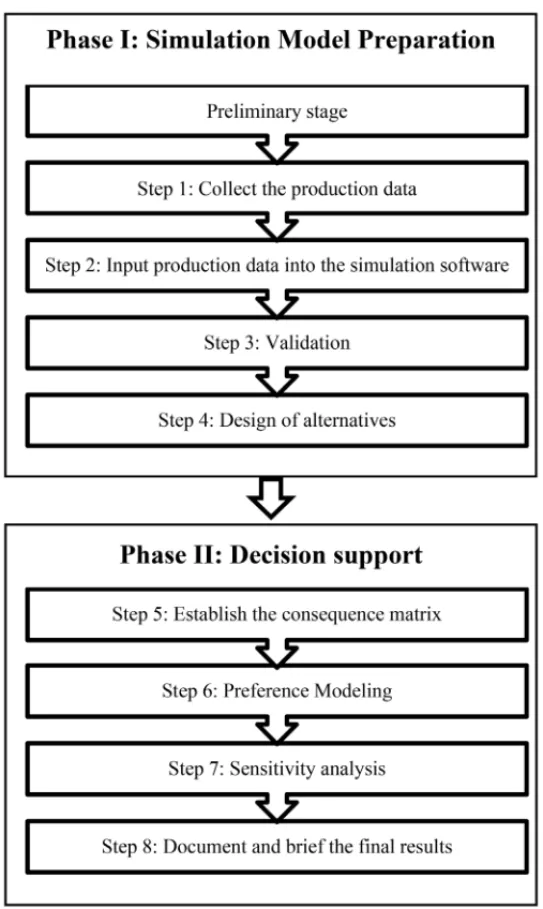
This section describes a framework (de Almeida, 2013a; de Almeida et al., 2015a) that is used to build multicriteria decision models on the basis of constructs obtained from the context of the decision problem itself. This framework allows the main characteristics of the method for developing simulation experiments proposed by Law & Kelton (2000) and the MAVT compen-satory approach (Keeney & Raiffa, 1976; de Almeida et al., 2015a) to be incorporated into a multi-attribute decision approach. An adaptation of that framework, with details of the current application, is presented in Figure 1. The proposed model assumes that there is a single DM with a mutual preference independence condition amongst the criteria (Keeney & Raiffa, 1976).

(3)

Figure 1– Proposed multi-attribute model.

MTS/CONWIP production system required by the proposed model, whereas the decision analyst gives methodological support so that the proposed model can be applied. Furthermore, the actors must reach a consensus on the set of decision attributes that will be applied to evaluate the alternatives. Due to the characteristics of the problem, we consider TH, CT, HC and SC as the most relevant decision attributes for our investigation.

(4)

should be validated in accordance with a structured technique (see Law & Kelton, 2000; Murray-Smith, 2015).

At Step 4, the set of alternatives A is developed based on WIP and FGI. This step also includes the simulation runs with set Aconsidering the experimental parameters: number of replications R and warm-up conditions. Thereafter, the consequence matrix is established to represent the performance of each alternativeai ∈ A= {a1,a2, . . . ,ai. . . ,an}over the attributes TH, CT, HC and SC. The procedure consists of calculating the average outcomexi j for each combination of one alternativeai and one attribute j, taking into account that the set of simulation outputsx is produced inRreplications.

Step 6 consists of obtaining the subjective information from the DM within the axiomatic struc-ture of MAVT. This preference modeling is assisted by a web-based DSS (de Almeida et al., 2015b) that performs the classical trade-off elicitation protocol proposed by Keeney & Raiffa (1976). This DSS was developed by CDSID (Center for Decision Systems and Information De-velopment), which CDSID can made available on request (www.cdsid.org.br).

After inputting the required data set into the DSS, a sequence of questions is put to the DM, in order to obtain the indifference values between pairs of consequences associated to ordered attributes. The first group of questions is designed to rank the attribute weights. Then, other questions allow the DM to understand the consequence space. Finally, the DM should express the indifference value between pairs of consequences related to the ranking of attributes. As a result, the scaling constantskj are obtained and used to aggregate the DM’s tradeoff judgments into a multi-attribute value function (1).

v(ai)=kC TVC T(ai)+kT HVT H(ai)+kH CVH C(ai)+kSCVSC(ai) (1)

wherev(ai)is the overall value of alternativeaiandVj(ai)represents the normalized value of a simulated consequence for attributej. The following property holds (2):

kC T +kT H+kH C+kSC=1. (2)

The use of the additive form in (1) relies on the assumption that DM’s preferences over some attribute are not influenced by the level of another attribute (the mutual preference independence condition).

At step 7, the sensitivity analysis verifies to what extent the ranking of alternatives obtained by applying (1) is sensitive to variations in the scaling constants from the multi-attribute function in (1). For this purpose, a Monte Carlo simulation and a Kendaltrank correlation (Kendall, 1970) are applied to test the null hypothesis(h0)that there is no correlation between each new ranking and the original one,h0:τ =0.

(5)

3 DECISION MODEL APPLICATION

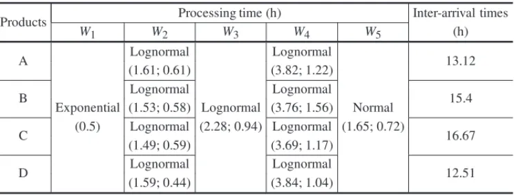
The case under investigation is an MTS/CONWIP multi-product manufacturing line of a met-alwork company. This system consists of five workstationsWh(h = 1, . . . ,5)with a stable bottleneck and a storage area. In the storage area, finished products await orders from customers. If there are finished goods that match orders, the goods are dispatched to customers and this information is sent toW1so as to update the planned order release. When the WIP falls below the target level, a product type is released to the system in accordance with the FIFO (first-in, first-out) dispatching rule. All product types (A, B, C and D) are manufactured in batch quanti-ties. The statistical parameters of processing times and the inter-arrival time of customer orders are summarized in Table 1.

Table 1– Summary of processing times and inter-arrival times.

Products Processing time (h) Inter-arrival times

W1 W2 W3 W4 W5 (h)

A

Exponential

Lognormal

Normal

13.12

(0.5)

(1.61; 0.61)

(2.28; 0.94)

(3.82; 1.22)

(1.65; 0.72)

B Lognormal Lognormal 15.4

(1.53; 0.58) (3.76; 1.56)

C Lognormal Lognormal 16.67

(1.49; 0.59) (3.69; 1.17)

D Lognormal Lognormal 12.51

(1.59; 0.44) (3.84; 1.04)

The plant works three 7-h shifts a day, five days per week and is idle during the weekend unless on-request. In relation to the simulation experiment, the following assumptions were made:

• There is an infinite supply of raw materials.

• WorkstationW4is the only bottleneck in the entire line.

• Transfer time between workstations is negligible.

• The scheduling of orders in the system is based on the FIFO rule.

• The holding cost per product-type is determined by multiplying the average of inventory-on-hand by an associated unit holding cost. Then, HC is determined as the sum of these partial values.

• The stockout cost is determined by multiplying the number of canceled orders by the invariant gross profit yielded by each customer order.

(6)

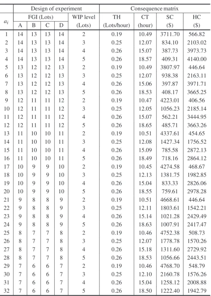
To validate the model, the comparison between the CT in the simulated period was considered. Adhesion between the real and the simulated system represented 86.1%. Considering the inter-arrival time of orders and the capacity of the storage unit, the simulation model was used to run different combinations of FGI and WIP. Trial runs reveal that 32 alternatives are necessary to explore the tradeoffs amongst criteria. Each treatment consists of 30 runs and the results were collected over 1680 hours (70 days of operations). The data from an initial warm-up period of 24 hours were discarded. After making pilot runs, the consequence matrix was established to represent the average performance value of each combination of alternativeai and attribute j. Table 2 shows the alternatives, their evaluation, and the consequence matrix.

As can be observed in the consequence matrix (Table 2), increasing the WIP level from 2 to 4 lots results in a better performance at TH. However, the CT performance is reduced. Likewise, increasing WIP from 4 to 5 lots does not yield a better consequence for TH and the performance of CT is the worst.

This performance behavior of MTS/CONWIP systems can be explained by Little’s Law (Little, 1961). In addition, alternatives that propose a WIP level of 2 lots yield the highest SC value, due to the low level of the use of capacity. However, these alternatives provide the lowest HC value. Alternativesa3,a4,a7,a8anda12 provide the most satisfactory performance for the SC attribute, while producing an extra holding cost in comparison to the alternatives associated with lower levels of FGI.

Assuming a DM with the mutual independence condition amongst criteria, the MAVT approach is applied in order to deal simultaneously with the conflicting nature of the decision attributes. After MAVT concepts have been explained to the DM, an assessment is made of his preferences by using the web-based DSS. This process starts by including the basic inputs to web-DSS, namely: problem description, the set of attributes, preference direction to each attribute j (maxi-mization or mini(maxi-mization) and consequence matrix. Subsequently, the rank-order of the weights of the attributes is elicited, using questions like: “consider a hypothetical alternative, with the worst performance in all criteria, and suppose you have to choose it. Now suppose that you can improve the performance of this alternative in only one of the criteria to the maximum value, which criterion would you choose?” As a result, the order obtained was: SC, HC, TH and CT.

After the ranking of criteria weights, the DSS provides a graphical visualization of the range of the consequences space[x0_j;x∗_j], wherex0_j andx∗_j are the worst and the best outcomes respec-tively. At this point, other questions are put to the DM in order to provide a better understanding of the consequence space. Thereafter, the elicitation ofkj begins by asking the DM for indiffer-ences between two consequindiffer-ences

x1=x∗SC,x0H C,xT H0 ,xC T0

and x2=x0SC,x∗H C,xT H0 ,x0C T

(7)

Table 2– Configuration of alternatives and consequence matrix.

Design of experiment Consequence matrix

ai FGI (Lots) WIP level TH CT SC HC A B C D (Lots) (Lots/hour) (hour) ($) ($) 1 14 13 13 14 2 0.19 10.49 3711.70 566.82 2 14 13 13 14 3 0.25 12.07 834.10 2103.02 3 14 13 13 14 4 0.26 15.07 387.73 3973.73 4 14 13 13 14 5 0.26 18.57 409.31 4140.00 5 13 12 12 13 2 0.19 10.49 3807.97 446.64 6 13 12 12 13 3 0.25 12.07 938.38 2163.11 7 13 12 12 13 4 0.26 15.06 397.87 3971.71 8 13 12 12 13 5 0.26 18.53 408.17 3665.25 9 12 11 11 12 2 0.19 10.47 4223.01 406.56 10 12 11 11 12 3 0.25 12.05 1056.23 2185.14 11 12 11 11 12 4 0.26 15.07 562.21 3444.95 12 12 11 11 12 5 0.26 18.65 485.71 3663.26 13 11 10 10 11 2 0.19 10.51 4337.61 454.65 14 11 10 10 11 3 0.25 12.08 1427.34 1756.52 15 11 10 10 11 4 0.26 15.09 785.58 2872.13 16 11 10 10 11 5 0.26 18.49 718.16 2864.12 17 10 9 9 10 2 0.19 10.45 4274.58 468.67 18 10 9 9 10 3 0.25 12.13 1381.75 1982.85 19 10 9 9 10 4 0.26 15.04 833.33 2826.06 20 10 9 9 10 5 0.26 18.55 759.61 2978.28 21 9 8 8 9 2 0.19 10.51 4668.61 446.64 22 9 8 8 9 3 0.25 12.11 1803.61 1542.21 23 9 8 8 9 4 0.26 15.14 1021.28 2429.49 24 9 8 8 9 5 0.26 18.63 1007.91 2417.47 25 8 7 7 8 2 0.19 10.46 4752.38 508.73 26 8 7 7 8 3 0.25 12.07 1778.78 1570.26 27 8 7 7 8 4 0.26 15.18 1311.60 2729.92 28 8 7 7 8 5 0.26 18.53 1056.66 2443.51 29 7 6 6 7 2 0.19 10.46 4768.70 548.79 30 7 6 6 7 3 0.25 12.10 2160.78 1576.26 31 7 6 6 7 4 0.26 15.04 1258.12 2008.88 32 7 6 6 7 5 0.26 18.50 1222.40 1942.79

to the classical tradeoff method (see Keeney & Raiffa, 1976; de Almeida et al., 2015a). Following this elicitation procedure, the values ofkj obtained were:

kSC =0.396,kH C =0.297, kT H =0.223 and kC T =0.084.

(8)

Table 3– Ranking of alternatives.

Rank ai v(ai)

1 2 0.776

2 6 0.762

3 14 0.750 4 10 0.750 5 31 0.747 6 18 0.736 7 23 0.734 8 26 0.733 9 22 0.733 10 15 0.720 11 19 0.720 12 32 0.720 13 24 0.700 14 30 0.698 15 11 0.695 16 28 0.695 17 16 0.693 18 27 0.683 19 20 0.679

20 3 0.669

21 7 0.668

22 8 0.656

23 12 0.648

24 4 0.618

25 5 0.464

26 1 0.463

27 9 0.430

28 17 0.421 29 13 0.415 30 21 0.386 31 25 0.374 32 29 0.369

v(ai)is the overall value of alternativeai.

(9)

the cost associated with lost sales in $3,388.91 in relation toa2. Since there is no alternative providing the best results in all attributes modeled, the use of MAVT allows a compensating disadvantage in one of the performance attributes because of an advantage in other attributes, taking into account the goals that the DM wants to achieve.

A sensitivity analysis was conducted in order to examine the robustness of the compromise solu-tion as to variasolu-tions in the scaling constants. For this purpose, 10,000 independent ranks of alter-natives were randomly generated from a uniform distribution with parameters(1−20%)kj and

(1+20%)kj, wherekj is the scaling value elicited previously. Simulation results are summarized as follows:τ (max)=1,τ (min)=0.95,τ (mean)=0.98,τ (median)=0.99,τ (mode)=0.99,

τ (standard deviation) = 0.013. The p-value of 0.078 was not statistically significant at a 5% level of significance. Thus, we can infer that the compromise solutiona2remains in first position in the ranking, since the simulated and the original ranks are independent. Although the com-promise solution remains invariant within the(±20%)range, this does not mean thatkj can be elicited without careful evaluation of the mutual preference independence condition. In addition, the proposed MAVT model should be applied to MTS/CONWIP decision problems when the DM wishes to make compensations among multiple conflicting attributes. These can be obtained by the model given in (1). For situations in which the DM seeks to maximize the performance of the MTS/CONWIP system for a single objective, classical optimization approaches can be considered.

Due to the compensatory nature of MAVT, the values of the scale constants cannot be simply interpreted as a relative degree of importance of the attributes. The determination ofkj is based on subjective information provided by the DM, considering the range of the consequences space. That is, when the range[x0_j;x∗_j]changes, it is necessary to adjust the value ofkj. For instance, by varying the values of the consequence matrix shown in Table 2 within the range(1−25%)xi j and(1+25%)xi jwithout adjustingkj, the Kendall tau test rejectsh0:t =0 (p-value of 0.034), which indicates significant differences between ranks evaluated at a 5% level of significance. This feature is a distinctive feature of this multi-attribute model in relation to the models proposed hitherto. However, the proposed model assumes that the DM is willing to answer all questions required by the tradeoff method (Keeney & Raiffa, 1976).

To address the uncertainties of the performance of the MTS/CONWIP system, Pergher and de Almeida (2017) integrated discrete event simulation with Multi-attribute Utility Theory – MAUT (Keeney & Raiffa, 1976). Nonetheless, this paper assumes that the average value of consequences provides a satisfactory representation of the performance of the system and hence the use of MAVT is suitable in this context.

4 CONCLUDING REMARKS AND FUTURE RESEARCH

(10)

We use a web-based DSS developed by the CDSID to implement the MAVT compensatory approach. The solution recommended for this multi-attribute problem isa4, which reflects the DM’s tradeoff judgment among multiple conflicting attributes.

The use of a discrete event simulation and MAVT allows not only the economic results to be evaluated but also those intangible consequences yielded by the level of WIP and FGI, without stopping the real system.

The proposed model can be further improved, for example by considering the additive-veto model (de Almeida, 2013b). For decision problems where the DM does not wish to select one alternative with a very low performance in one attribute, even though it is compensated by the high level of one or more of the other attributes, additive-veto models can be employed.

ACKNOWLEDGMENTS

This work had partial support from CNPq (Conselho Nacional de Desenvolvimento Cient´ıfico e Tecnol´ogico), the Brazilian Research Council. The CNPq was not involved in the study or in writing this paper.

The authors would like to thank the Editor and the anonymous reviewers for their insightful critique of an earlier version of this paper and for their valuable suggestions for improving it.

REFERENCES

[1] DEALMEIDAAT, CAVALCANTECAV, ALENCARMH, FERREIRARJP,DEALMEIDA-FILHOAT & GARCEZTV. 2015a. Multicriteria and Multi-objective Models for Risk, Reliability and Mainte-nance Decision Analysis. International Series in Operations Research & Management Science. New York: Springer.

[2] DEALMEIDAAT, LUGOSDR, DOWSLEYBS, SANTOSVAPA & CLEMENTETRN. 2015b. Elicita-tion for Tradeoff Additive Model with Linear or Non-Linear Value FuncElicita-tion and Sensitivity Analysis – Web-based – C´odigo TU-T2OMO-WT1. Computational program developed by CDSID (Center for Decision Systems and Information Development). Registro INPI: BR5120160013214.

[3] DEALMEIDAAT. 2013a. Processo de Decisão nas Organizações. São Paulo: Atlas.

[4] DEALMEIDAAT. 2013b. Additive-veto models for choice and ranking multicriteria decision prob-lems.Asia-Pacific Journal of Operational Research,30(6): 1–20.

[5] BELTONV & STEWARTTJ. 2002. Multiple criteria decision analysis. Kluwer Academic Publishers. 372 pages.

[6] FONTANAME & CAVALCANTECAV. 2013. Electre tri method used to storage location assignment into categories.Pesquisa Operacional,33(2): 283–303.

[7] GONGQ, YANGY & WANGS. 2014. Information and decision-making delays in MRP, KANBAN, and CONWIP.Production Economics,156: 208–213.

(11)

[9] KEENEYRL & RAIFFAH. 1976. Decision Making with Multiple Objectives, Preferences, and Value Tradeoffs. New York: John Wiley & Sons. 592 pages.

[10] KENDALLMG. 1970. Rank Correlation Methods. 4 ed. London: Griffin.

[11] LAWAM & KELTONWD. 2000. Simulation modeling and analysis. 3rd ed. Boston: McGraw-Hill. 760 pages.

[12] LITTLEJDC. 1961. A Proof for the Queuing Formula: L=λW.Operations Research,9: 83–387.

[13] LUJ, YANGT & WANGC. 2011. A lean pull system design analyzed by value stream mapping and multiple criteria decision-making method under demand uncertainty.Computer Integrated,24(3): 211–228.

[14] MURRAY-SMITHDJ. 2015. Testing and Validation of Computer Simulation Models, Principles, Methods and Applications. Series: Simulation foundations, methods and applications. Springer: Cham. 252 pages.

[15] PERGHERI & DE ALMEIDA AT. 2017. A multi-attribute decision model for setting production planning parameters.Manufacturing Systems,42: 224–232.

[16] PERGHERI & VACCAROGLR. 2013. Work in process level definition: a method based on com-puter simulation and Electre tri.Produc¸˜ao,24(3): 536–547.

[17] RABELOL, ESKANDARIH, SHAALANT & HELALM. 2007. Value chain analysis using hybrid simulation and AHP.Production Economics,105(2): 536–547.

[18] SPEARMAN ML, WOODRUFF DL & HOPP WJ. 1990. Conwip: a pull alternative to Kanban.

Production Research,28(5): 879–94.