Optimizing base stock levels and profits of a two-echelon inventory problem with stochastic demand

Optimizing Base Stock Levels and Profits of a

Two-Echelon Inventory Problem with

Stochastic Demand

Kizito Paul Mubiru

Department of Mechanical and Production Engineering Kyambogo University,Uganda

Abstract - Planning and managing adequate base stock levels of items plays an important role in supply chain management to optimize profits. In this paper, a new mathematical model is developed to optimize base stock levels (BSL) of a two-echelon inventory system under demand uncertainty. The system consists of one factory warehouse at the upper echelon and four supermarkets at the lower echelon. Sales price and scheduled inventory replenishment periods are uniformly fixed over all echelons and demand at the supermarkets is stochastic and stationary. Adopting a Markov decision process approach, the states of a Markov chain represent possible states of demand for milk powder product. The replenishment cost, holding cost, shortage cost and sales price are combined with demand and inventory positions in order to generate the profit matrix of a given echelon. The matrix represents the long run measure of performance for the decision problem. The objective is to determine in each echelon of the planning horizon an optimal base stock level so that the long run profits are maximized for a given state of demand. Using weekly equal intervals, the decisions of how much to replenish are made using dynamic programming over a finite period planning horizon. A numerical example demonstrates the existence of an optimal state-dependent base stock level and profits over the echelons.

Keywords: Base stock level, Echelon, Inventory, Stochastic demand

I. INTRODUCTION

In practice, inventory may be stored at the point of manufacture (one echelon of inventory system), then at national or regional warehouse (a second echelon), then at field distribution centers (a third echelon) etc. Some coordination is needed to effectively manage base stock levels of the product at different echelons. Since the base stock level at each echelon (except the top one ) is replenished from the next higher echelon, the base stock level needed at the higher echelon is affected by how soon replenishment will be needed at the various locations for the lower echelon. To cope with current turbulent market demands, there is still need to adopt coordinated inventory control across supply chain facilities by establishing optimal base stock levels in a stochastic demand environment. In echelon-based inventory systems, industries continually strive to optimize base stock levels of products. Two major decisions ar usually encountered: (i) determining the optimal base stock level of the item in question that maximize profits (ii) Determining the optimal profits associated with a chosen base stock level under demand uncertainty.

According to Rodney and Roman [1], the optimal policies study in the context of a capacitated two-echelon inventory system. This model includes installations with production capacity limits, and demonstrates that a modified base stock policy is optimal in a two-stage system when there is a smaller capacity at the downstream facility. This is shown by decomposing the dynamic programming value function into value functions dependent upon individual echelon stock variables. The optimal structure holds for both stationary and non stationary customer demand. Derek and Iyogun [2] examined the problem of managing inventories where there is a joint fixed cost for replenishing plus an item-by-item fixed cost for each item included in the replenishment order. Due to the complexity of the optimal solution, attention is focused on fixed heuristics, and in particular ‘can-order’ or (s,c,S) policies. Fangruo C[3] illustrated effective policies in a two-stage serial inventory system with stochastic demand. An inventory system is considered where Poisson demand occurs at stage 1.

A new lower bound in the cost of the optimal policy is produced and a simple periodic policy is proposed.

Stage 1 replenishes its inventory from stage 2; which in turn orders from an outside supplier with unlimited stock. A fixed cost is incurred at stages 1 and 2 under the assumption that the supply lead time at stage 2 is zero. A simple heuristic policy is characterized where long-run average cost is guaranteed to be within 6% of optimality.

face stochastic demand and the system is controlled by continuous review installation stock policies with given batch quantities. A back order cost is provided to the warehouse and the warehouse chooses the reorder point so that the sum of the expected holding and backorder costs are minimized. Given the resulting warehouse policy, the retailers similarly optimize their costs with respect to the reorder points. The study provides a simple technique for determining the backorder cost to be used by the warehouse.

In related work by Haji R [5], a two-echelon inventory system is considered consisting of one central warehouse and a number of non-identical retailers.The warehouse uses a one-for-one policy to replenish its inventory, but the retailers apply a new policy that is each retailer orders one unit to central warehouse in a predetermined time interval; thus retailer orders are deterministic not random. In a similar context, Abhijeet S and Saroj K [6] considered vendor managed Two-Echelon inventory system for an integrated production procurement case. Joint economic lot size models are presented for the two supply situations, namely staggered supply and uniform supply. Cases are employed that describe the inventory situation of a single vendor supplying an item to a manufacturer that is further processed before it is supplied to the end user. Using illustrative examples, the comparative advantages of a uniform sub batch supply over a staggered alternative are investigated and uniform supply models are found to be comparatively more beneficial and robust than the staggered sub batch supply.

The literature cited provide profound insights by authors that are crucial in analyzing two-echelon inventory systems in a stochastic demand setting. However, a new dynamic approach is sought in order to relate state-transitions with customers, demand and price of item at the respective echelons so as to optimize replenishment policies and base stock levels in a multistage decision setting.

In this paper, a two-echelon production- inventory system is considered whose goal is to optimize replenishment policies and base stock levels associated with the inventory item. At the beginning of each period, a major decision has to be made, namely whether to replenish additional units of the item or not to replenish and keep the item at prevailing inventory position in order to sustain demand at a given echelon. The paper is organized as follows. After describing the mathematical model in §2, consideration is given to the process of estimating the model parameters. The model is solved in §3 and applied to a special case study in §4.Some final remarks lastly follow in §5.

II. MODEL FORMULATION

2.1 Notation and assumptions

i,j = States of demand F = Favorable state U = Unfavorable state h = Inventory echelon n,N = Stages

Z = Replenishment policy

NZ = Customer matrix

NZij = Number of customers

DZ = Demand matrix

DZij = Quantity demanded

QZ = Demand transition matrix

PZ = Profit matrix PZij = Profits

eZ

i = Expected profits

aZ

i = Accumulated profits

Bi = Base Stock Level

p = Unit sales price

n=1,2,……….N

classified as either favorable (denoted by state F) or unfavorable (denoted by state U) and the demand of any such period is assumed to depend on the demand of the preceding period. The transition probabilities over the planning horizon from one demand state to another may be described by means of a Markov chain. Suppose one is interested in determining an optimal course of action, namely to replenish additional units of the item (a decision denoted by Z=1) or not to replenish additional units of the item (a decision denoted by Z=0) during each time period over the planning horizon, where Z is a binary decision variable. Optimality is defined such that the maximum expected sales revenue is accumulated at the end of N consecutive time periods spanning the planning horizon under consideration. In this paper, a two-echelon (h =2) and two-period (N=2) planning horizon is considered.

2.2 Finite - period dynamic programming problem formulation

Recalling that the demand can either be in state F or in state U, the problem of finding an optimal base stock level and profits may be expressed as a finite period dynamic programming model.

Let Pn(i,h) denote the optimal expected profits accumulated during the periods n,n+1,…...,N given that the state of

the system at the beginning of period n is i F,U }.The recursive equation relating Pn and Pn+1 is

(1)

{F , U } , h={1,2} , n= 1,2,……….N together with the final conditions

PN+1(F , h ) = PN+1(U , h ) = 0

This recursive relationship may be justified by noting that the cumulative profits PZij(h)+ PN+1(j)

F, U F, U } at the start of period n occurs

with probability QZij(h).

Clearly, eZ(h) = [QZij(h)] [ PZ(h) ]T (2)

where ‘T’ denotes matrix transposition, and hence the dynamic programming recursive equations

(3)

PN(i, h) = maxZ {e Z

i(h)} (4)

result where (4) represents the Markov chain stable state.

2.2.1 Computing QZ(h) and PZ(h)

F, U F, U},given replenishment policy Z

may be taken as the number of customers observed over echelon h with demand initially in state i and later with demand changing to state j, divided by the sum of customers over all states. That is,

{F , U } = {1, 2} (5)

When demand outweighs on-hand inventory, the profit matrix PZ(h) may be computed by means of the relation

where p denotes the sales price,cr denotes the unit replenishment cost,ch is the unit holding cost and cs is the unit

shortage cost of item.

(6)

{ F, U }, and Z

The base stock level when demand is initially in state F, U

{ F, U },

III. OPTIMIZATION

The optimal base stock level and profits are found in this section for each period over echelon hseparately.

3.1 Optimization during period 1

When demand is favorable (ie. in state F), the optimal replenishment policy and base stock level during period 1 are

and

The associated profits are then

Similarly, when demand is unfavorable (ie. in state U ), the optimal replenishment policy and base stock level during period 1 are

and

In this case, the associated profits are

3.2 Optimization during period 2

Using (2),(3) and recalling that aZi(h)denotes the already accumulated profits at the end of period 1 as a result of

decisions made during that period, it follows that

and while the associated profits are

Similarly, when the demand is unfavorable (ie. in state U), the optimal replenishment policy and base stock level during period 2 are

and

In this case the associated profits are

IV. CASE STUDY

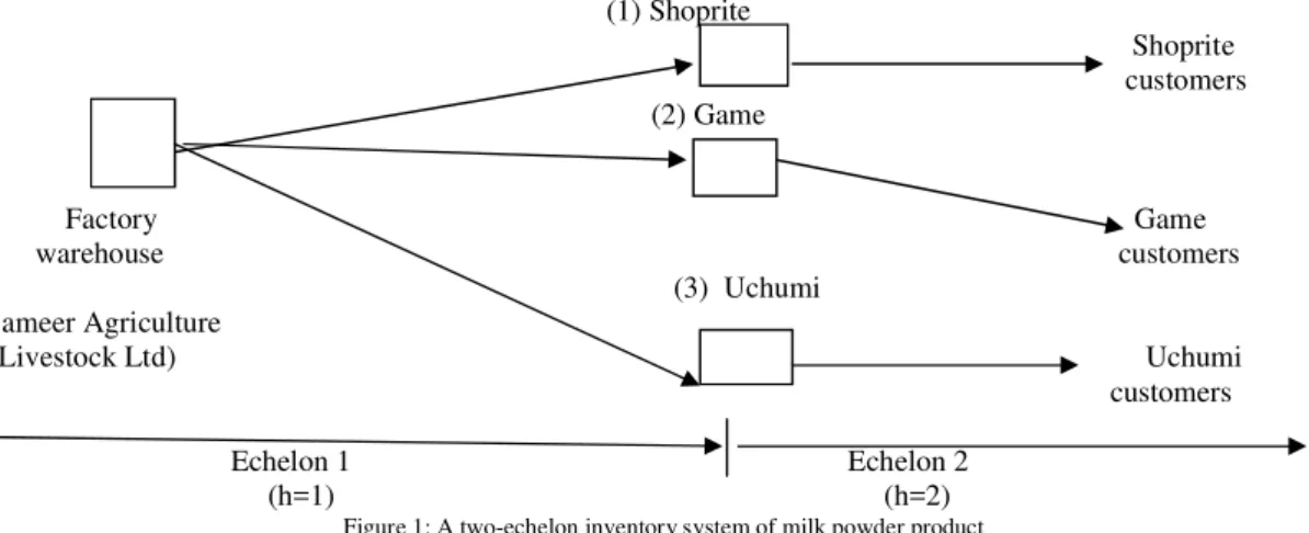
In order to demonstrate use of the model in §2-3, real case applications from Sameer Agriculture and LivestockLtd, a

production plant for milk powder and three supermarkets: Shoprite supermarket, Game supermarket and Uchumi

supermarket in Uganda are presented in this section. The production plant supplies milk powder at supermarkets (echelon 1), while end customers come to supermarkets for milk powder product (echelon 2).The demand for milk powder fluctuates every week at both echelons. The production plant and supermarkets want to avoid excess inventory when demand is Unfavorable (state U) or running out of stock when demand is Favorable (state F) and hence seek decision support in terms of an optimal base stock level and the associated profits of milk powder product in a two-week planning period. The network topology of a two-echelon inventory system for milk powder product is illustrated in Figure 1 below:

(1) Shoprite

Shoprite customers (2) Game

Factory Game warehouse customers

(3) Uchumi (Sameer Agriculture & Livestock Ltd) Uchumi

customers

Echelon 1 Echelon 2 (h=1) (h=2)

Figure 1: A two-echelon inventory system of milk powder product

4.1 Data collection

Table 1: Customers, Demand and replenishment policies and sales price (in UGX) given state- transitions, and echelons over twelve weeks

State transition (i,j) Echelon (h) Replenishment Policy (Z) Customers

NZij(h)

Demand

DZij(h)

Inventory

IZij(h)

Sales Price (p) FF FU UF UU 1 1 1 1 1 1 1 1 91 71 64 13 156 15 107 11 95 93 93 94 6000 6000 6000 6000 FF FU UF UU 1 1 1 1 0 0 0 0 82 30 55 25 123 78 78 15 43.5 45 46.5 45.5 6000 6000 6000 6000 FF FU UF UU 2 2 2 2 1 1 1 1 45 59 59 13 93 60 59 11 145 40 35.5 79.5 6000 6000 6000 6000 FF FU UF UU 2 2 2 2 0 0 0 0 54 40 45 11 72 77 75 11 81 78.5 79.5 78.5 6000 6000 6000 6000

At echelon 1, when additional units were replenished (Z=1),

When additional units were not replenished (Z=0),

At echelon 2, when additional units were replenished (Z=1),

When additional units were not replenished (Z=0),

4.2 Solution procedure for the two-echelon Base Stock Level(BSL)problem

respectively, for the case when additional units were replenished (Z=1) during week 1, while these matrices are given by

respectively, When additional units were not replenished (Z=0) during week 1.

When additional units were replenished (Z = 1), the matrices Q1 (1), P1(1) , Q1 (2) and P1(2) yield the profits (in million UGX)

However, When additional units were not replenished (Z=0), the matrices Q0 (1), P0(1) , Q0 (2) and P0(2) yield the profits (in million UGX)

When additional units were replenished (Z = 1), the accumulated profits (in million UGX) for each respective echelon follow:

Echelon 1:

Echelon 2:

When additional units were not replenished (Z = 0), the accumulated profits (in million UGX) follow:

Echelon 1:

Echelon 2:

Week1: Echelon 1

Since 184.38 > 110.70, it follows that Z=0 is an optimal replenishment policy for week 1 with associated profits of

184.38 million UGX and Base Stock Level [BF (1) = 95+93 = 188 packets ]for the case of favorable demand. Since

183.09 > 95.105, it follows that Z=1 is an optimal replenishment policy for week 1 with associated profits of

183.09million UGX and Base Stock Level [BU (1) = 107+11 = 118 packets] for the case when demand is

unfavorable.

Week1: Echelon 2

Since 199.84 > 107.46, it follows that Z=0 is an optimal replenishment policy for week 1 with associated profits of

199.84 million UGX and Base Stock Level [BF (2)= 145+40=185 packets] when demand is favorable. Since 198.26

> 30.09, it follows that Z=0 is an optimal replenishment policy for week 1 with associated profits of 198.260 million

UGX and Base Stock Level [BU (2) = 35.5+79.5=115 packets] if demand is unfavorable.

Week 2: Echelon 1

Since 368.4 > 294.51, it follows that Z=0 is an optimal replenishment policy for week 2 with associated profits of

368.4 million UGX and Base Stock Level [BF (1)= 145+40 =185 packets ]when demand is favorable. Since 367.25

> 279.08, it follows that Z=1 is an optimal replenishment policy for week 2 with associated accumulated profits of

367.25 million UGX and Base Stock Level [BU(1)= 59+11=70 packets ]if demand is unfavorable.

Week 2: Echelon 2

Since 390.13 > 301.7, it follows that Z=0 is an optimal replenishment policy for week 2 with associated

accumulated profits of 390.13 million UGX and Base Stock Level [BF (2) = 145+40=185 packets ] when demand is

favorable. Since 385.37 > 216.98, it follows that Z=0 is an optimal replenishment policy for week 2 with associated

profits of 0.986 million UGX and Base Stock Level [BU(1)= 59+11 =70 packets ]if demand is unfavorable.

V. CONCLUSION

A two-echelon inventory model with stochastic demand was presented in this paper. The model determines an optimal base stock level and profits of a given item with stochastic demand. The decision of whether or not to replenish additional units is modeled as a multi-period decision problem using dynamic programming over a finite planning horizon. Results from the model indicate promising results pertaining to optimal base stock levels and profits over the echelons for the given problem. As a profit maximization strategy in echelon-based inventory systems, computational efforts of using Markov decision process approach provide promising results. It would however be worthwhile to extend the research and examine the behavior of base stock levels and profits under non stationary demand conditions over the echelons. In the same spirit, the model raises a number of salient issues to consider: Lead time of milk powder during replenishment and customer response to abrupt changes in price of the product. Finally, special interest is sought in further extending our model by considering base stock levels and profits in the context of Continuous Time Markov Chains (CTMC).

REFERENCES

[1] Rodney P & Roman K, 2004,”Optimal Policies for a capacitated Two-Echelon Inventory system”,Operations Research,152(5),739-747. [2] Derek R,Iyogun & Paul O,1998,”Periodic versus can-order policies for coordinated muti-item inventory systems”, Management

Science,34(6),791

[3] Fangruo C,1999,”94%-Effective policies for a two-stage serial Inventory System with Stochastic Demand”, Management Science,45(12),1679-1696.

[4] Axsater S, 2005, “A simple decision rule for decentralized two-echelon inventory control”, International Journal of Production Economics, 93-94(1), 53-59.

[5] Haji R & Tayebi H,2011,”Applying a new ordering policy in a two-echelon inventory system with poisson demand rate retailers and transportation cost”, International Journal of Business Performance and Supply chain Modeling,20-27.