A disruption production model with exponential demand

(1)

International Journal of Industrial Engineering Computations 3 (2012) 607–616 Contents lists available at GrowingScience

International Journal of Industrial Engineering Computations

homepage: www.GrowingScience.com/ijiec

A disruption production model with exponential demand

U. K. Khedlekar

Department of Mathematics and Statistics, Sagar Central University, Sagar M.P. India, 470003

A R T I C L E I N F O A B S T R A C T

Article history:

Received 25 January 2012 Accepted March, 10 2012 Available online 14 March 2012

In general, production system often gets disrupted due to uncertainty and un-planned events, which also affect demands resulting in less abet-margin of a company. With disrupted production system, management would need to study the variation of demand pattern and disruption of system; we have attempted an effort to establish an exponential demand with the disrupted production system and solved analytically the problem to determine production time before and after disruptions. Exponentially demand pattern studied, and also we simulate the results for sensitivity analysis in order to find which parameter is getting significant change for the proposed model.

Keywords:

Inventory

Disrupted Production System, Deterioration

Optimal Time

1. Introduction

Control and maintenance of the production system have attracted much attention of inventory managers. There are many reasons for disruptions of the production system like machine breakdown, unexpected events or some crises. An oil drilling company may be disrupted due to electricity supply, failure of drilling machines whereas oil refining company faces some problem of crude oil supply and availability of other raw materials or due to earthquake and strike. Lin and Kroll (2006) solved the production problem under an imperfect production system subject to random breakdowns.

(2)

608

rate for the newly launched deteriorating item. Joglekar (2003) used a linear demand function with price sensitiveness and allowed retailers to use a continuous increasing price strategy in an inventory cycle. He derived the retailer’s optimal profit by ignoring all the inventory costs. His findings are restricted to growing market only, which is neither for stable market nor for a declining market.

Joglekar (2003) used a linear demand function with price sensitiveness and allowed retailers to use a continuous increasing price strategy in an inventory cycle. He derived the retailer’s optimal profit by ignoring all the inventory costs. His findings are not restricted to growing market only, which is neither for stable market nor for a declining market. By dividing the demand rate into multiple segments, Shukla and Khedlekar (2010) introduced three-component demand rate for the newly launched deteriorating item. Qi, Bard and Yu (2004) analyzed the supply chain-coordination with demand disruption in a deterministic scenario. Expenditure sources like ordering cost, safety features, lead time and numbers of lots are the integral parts of decision making. An integrated inventory model focusing on these issues and aspects has been discussed by Lo (2007).

Giri et al. (1996) who computed the optimal policy of an EOQ model with dynamic costs. The model they proposed is very basic though, since they have considered the very special case where the holding and ordering costs are linear functions of time. The other shortcoming of that paper is that the deterioration rate is also a linear function of time, and the algorithm they proposed in order to solve the problem is only valid as long as the demand rate is a linear function of time.

Samanta and Roy (2004) studied a number of structural properties of the inventory system analytically by determination of production cycle time and backlog for deteriorating item, which follows an exponential distribution. They (2010) obtained optimal production time to facilitate the manufacturer sell the item in multiple markets by considering constant demand rate, but they do not readjust the production system. Due to above contribution time dependent demand is influenced to consider for deteriorating item and adjust the disrupted production system with shortages and when it occurs an optimal time of placing an order is obtained along with order quantity from the spot market. A central policy presented by Benjaafar EIHafsi (2006) specify a single product assemble-to-order system for my components, an end–product to serve and customer classes and problem solved as a Markov decision process and characterize the structure of an optimal policy. We refer some useful contribution to reader Balkhi and Bakry (2009), AI –Majed (2002), Khedlekar and Agarwal (2009), Mishra and Mishra (2010) and Shukla et al. (2012).

2. Assumptions and notations

Suppose that a deteriorating item manufactured by a single manufacturer and then sold to customers, the demand arising from the market is exponentially at a rate µect, the production rate is constant at a rate p > µ in each cycle; due to this inventory accumulate at a rate p -µect. If the production stopped at the time (Tp) and thus there after inventory depicted due to the demand and deterioration. During production disruption, if shortages occur, then it ordered from the spot market once in a cycle.

H Time horizon,

P Production rate,

θ Rate of deterioration,

µ Initial demand of item,

(3)

Td Production disruption time when system get disruptions,

Tpd New production time after system get disruptions,

Tr Time of placing the order when shortages occur,

Qr Order quantity (shortages) for placing the order when shortage occurs.

3. The production model without disruption

To compare the model output first, management optimizes the production system run without disruption with production rate p (per unit time) stopped at production time Tp and there after till time H, inventory depicted due to demand rate µect and deterioration rate θ of items (see fig. 1). The presentations in differential equations for two periods [0, Tp] and [Tp, H] satisfy throughout its domain.

Fig. 1. (Normal Production System without disruption)

( )

_{( )}

1

θ -μ ct

dI t

I t p e

dt + = ,

0 ≤ ≤

t

T

pboundary condition

I

1

( )

0 =

0

(1)

( )

_{( )}

2

θ -μ ct

dI t

I t e

dt + = ,

T

p

≤

t

≤

H

boundary condition I2

( )

H =0

(2)

On solving equation (1) and (2) with boundary conditions we get

( )

(

-

)

(

-

)

1 1 - -

-θt ct θt

p μ

I t e e e

θ c +θ

= (3)

( )

(

( )

)

2

c + θ H -θt ct

μ

I

t =

e

- e

c +

θ

(4)

As per fig. 1 inventory level I1(t) and I2(t) are equal at time Tp

i.e. I1(Tp) = I2(Tp) yields

1 log

cH H

p

Pc

θ

P -

θμ θμ

e

T

θ

Pc

P

θ

θ +

+

=

+

(5)

If θ <<1, then

H

Inventory

0

_T

p

(4)

610

(

1

)

cH

p cH

μe θH -μ T

Pc Pθ-μθ μe

+ =

+ +

(6)

4. The production model with disruption

In section 3 production rate unchanged but in practice production system is always disruption due to unplanned and thus we consider the production system little changed by ΔPand disruption time is Td. IfΔP<0, then production rate decreases and, if ΔP>0then production rate increases.

Lemma 1. If

(

)

-θH

(

)

(

cH -H θ

)

(

)(

θTd -Hθ

)

-e

θ

c / -e

e

μθ θ

c -P e

θ

c P

ΔP ≥ + + + + 1 then

manufacturing system still satisfies the exponential demand even production system has been disrupted,

otherwise If

(

)

-θH

(

)

(

cH -H θ

)

(

)(

θTd-Hθ

)

-e

θ

c / -e

e

μθ θ

c -P e

θ

c P

ΔP

-P ≤ ≥ + + + + 1 then

production system unable to satisfy exponential demand that is there will be shortages due to production disruption.

Proof: Suppose the production system disrupted at time Td as (see Fig. 2) and there after the production rate will be P+ΔP thus presentations of two differential equations for intervals [0, Td] and [Td, H] are

( )

_{( )}

1

θ -μ ct

dI t

I t p e

dt + = ,

0 ≤

t

≤

T

d boundary condition I1

( )

0 =0 , 0<θ <1

(7)

( )

_{( )}

2

θ -μ ct

dI t

I t P P e

dt + = + Δ ,

T

d

≤

t

≤

H

,

(8)

with boundary condition 1

( )

2

( )

(

1 - -

)

-

(

- -

)

d d d

θT cT θT

d d

p μ

I T I T e e e

θ c +θ

= =

On solving Eq. (8) with boundary condition we get

( )

(

-

)

(

)

(

)

2 1 - 1

-d

θT -θt

θt -θt ct

P P μ

I t e e + e - e

θ θ c+θ

Δ

= + (9)

If I2(H )≥0this means production system satisfy the exponential demand of items

That is

(

)

(

)

(

)

(

)

(

θTd-Hθ

)

θ

-H cH

-θH

-e

θ

c

-e e

μθ θ

c -P e

θ

c P

ΔP

1 +

+ + +

≥ then still satisfy the demand

(5)

That is ( ) ( )

(

)

( )

(

θTd-Hθ

)

H

θ

-cH

θH

--e

θ

c

-e e

μθ θ

c -P e

θ

c P

ΔP -P

1 +

+ + +

<

≤ then there will be shortages in the system.

This proved the lemma*

Again, if I2( )H ≥0then we find optimal production time (with disruption)

d p

T such that at time H entire

stock will be sold-out and inventory level will be zero.

If I₂( )H <0 there will be shortages in the system and in this situation we will find the optimum time Tr of placing the order and respective order quantity Qr.

Lemma 2. If I2( )H ≥0then production time with disruption

d p

T is obtained by

(

)

(

)(

)

d

θT cθ Hθ Pc+Pθ-μθ ΔP c+θ e +μθe

P+ΔP c+θ

d p θT

e

+

= (10)

Proof: If I2( )H ≥0

or

(

)

(

)

(

)

(

)

(

θTd -H θ

)

H

θ

-cH

-θH

-e

θ

c

-e e

μθ θ

c -P e

θ

c P

ΔP

1 +

+ + +

≥ that is on hand inventory is I2( )H

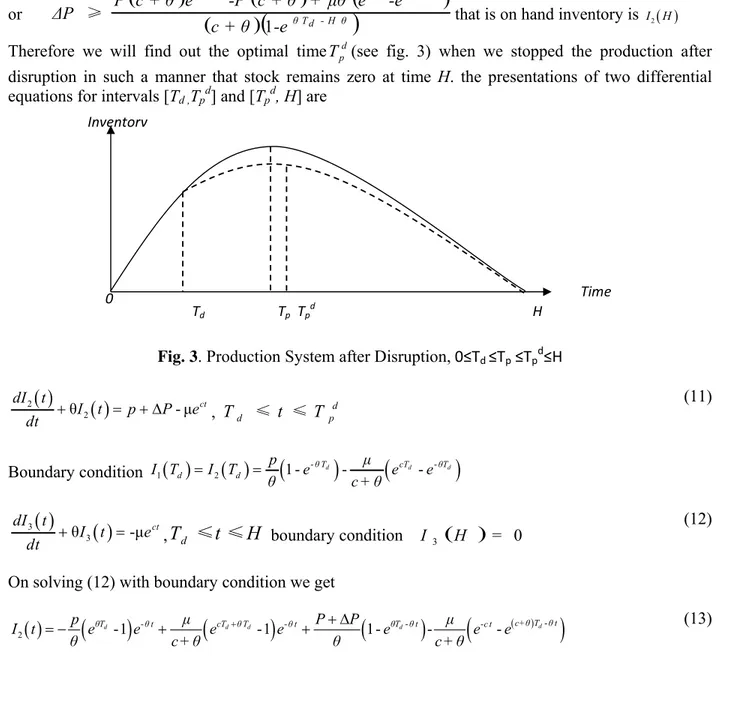
Therefore we will find out the optimal timeT_pd(see fig. 3) when we stopped the production after disruption in such a manner that stock remains zero at time H. the presentations of two differential equations for intervals [Td ,Tpd] and [Tpd, H] are

Fig. 3. Production System after Disruption, 0≤Td ≤Tp ≤Tpd≤H

( )

_{( )}

2

θ -μ ct

dI t

I t p P e

dt + = + Δ ,

d p

d t T

T ≤ ≤ (11)

Boundary condition 1

( )

2

( )

(

1 - -

)

-

(

- -

)

d d d

θT cT θT

d d

p μ

I T I T e e e

θ c +θ

= =

( )

_{( )}

3

θ -μ ct

dI t

I t e

dt + = ,

T

d

≤

t

≤

H

(

H

)

= 0

(12)

On solving (12) with boundary condition we get

( )

(

)

-

(

)

-

(

-

)

(

- ( ) -

)

2 -1 -1 1 - -

-d

d d d d c+θT θt

θT θt cT θT θt θT θt c t

p μ P P μ

I t e e e e e e e

θ c +θ θ c +θ

+ + Δ

= − + + (13)

Td Tp Tp

d

H

Time

Inventory

0

(6)

612

( )

(

-

)

3

-cH θH θt c t

μ

I t e e

c +θ

+

=

Using condition 2( ) 3( )

d d

p p

I T =I T

₍

(

₎₍

)

₎

d

θT cθ Hθ

Pc+Pθ-μθ ΔP c+θ e +μθe

P+ΔP c+θ

d p θT

e

+

= _■

Therefore increases in Td leads the production time with disruption Tpdincreases that is reduced incurred cost.

Lemma 3. If I2( )H <0then replenishment time Tr and order quantity Qrare

_e-θTr

(

_Pc+_Pθ μθ- + Δ_{P c}

(

+θ

)

_eθTd

)

+μθ_ecTr +

(

_P+Δ_{P c}

)(

+θ

)

=0

( )

(

- Tr

)

(

cH H- Tr

)

3 1-e - - e

r

θHθ c T θ θ

r r

P P μ

Q I T e

θ c +θ

+ + Δ

= = (14)

Proof: If I2( )H <0 then production system does not fulfill the exponential demand

Or

(

)

₍

₎

(

₍

)

₎

(

)

1 d

-θH cH -θH

θT - Hθ

P c θ e - P c θ μθ e - e -P ΔP

c θ - e

+ + +

≤ <

+

C

that is there will be shortages in the system.

Suppose Tr and Qr (see Fig. 4) are time of placing an order and order quantity respectively.

Fig. 4. (Production System after Disruption, Tpd = H)

Then I2(Tr)=0 (by Eq. (14)

r

cT

ΔP-P μ

+ e -

-θ c+θ

θT d

r r θT

θT μ P ΔP

e e

c +θ θ θ

+

⎛ ⎞

=

⎜ ⎟

⎝ ⎠

(15)

or -

(

)

(

)(

)

- d 0

r θT r

θT cT

e Pc+Pθ μθ+ ΔP c+θ e +μθe + P+ΔP c+θ =

Then presentation of differential equation in this situation is

( )

_{( )}

3

θ -μ ct

dI t

I t P P e

dt + = + Δ ,

T

r

≤

t

≤

H

( )

H =0

(16)

Above equation gives

Td Tp Tr Tp d

= H

Time

Inventory

0

(7)

Hen r Q 5. A For =8 Fol Ca Fro mo sam

nce the orde

( )

3 r I T = = Application r application on applying llowing figur

se I: When

Fig.

om Fig. 5, Tp ore manufact me followed

I3

( )

t =

er quantity is

(

1-e

P P

θ

+ Δ

and sensiti

n we assumed g then we get

res shows se

ΔP

-P ≤ <

. 5. (Tp with

7. (Tr with r

Tp is increasin turer items.

by Fig. 6.

(

1

P P

θ

+ Δ =

s Qr= I3(Tr)

)

r

- T eθH θ - μ

c +

ive Analysis

d a particula t I2(H)>0 an ensitiveness ( )

(

-θ e θ c P + repective to

repective to T

ng inθ prod So it is the

)

--eθH θt

-c

(

cH - e r c T μ e θ + s

ar case when nd thus by eq with respect ( ) H θ _θ c P - + θ)

Td)

duction time effective w

(

μ

-r

cT c H

e e θ +

)

r H- T θ θ +

n P=350, µ= quation (6) a

tive theθ an

(

cH

--e e

μθ +

is direct pro way to reduce

)

-H+θH θt

■

200, ΔP=-2 and (11) Tp= nd Td.

)

( )

H

θ _/ _c ₊_θ

Fig. 6. ( d p

T

Fig. 8. (Qr w

oportional to e the cost as

00, θ=.03, c 12.83 d 1

p

T =

)

(

θTd-Hθ

)

-e

1

with repecti

with repectiv

o deterioratio s keeping lo

c=0, H=20 a 8.3578.

ive to Td)

ve to Td)

on means it ower deterior

(17)

and Td

(8)

614

If I ma disr by Ca Fro rep Tab Com Par 0 0.0 -0.0 0.0 -0.0 0.1 -0.1 0.1 -0.1 As tha valu

I2(H) < 0 the rket at time ruption time Fig. 8.

se II: When

om Fig. 9 ti production ea ble 1 mparison wi rameter ‘c’ 2 02 5 05 0 10 5 15

per Table 1 n constant, w ue of c, I2(H

en there are s Tr (Fig. 7) W e produces fe

n ΔP>

(

P c( +θ

ime d p

T decr

arlier.

ith constant / Demand Trend Constan Increasin Decreasi Increasin Decreasi Increasin Decreasi Increasin Decreasi

, one can ob whenever c H) is negati

shortages occ Which decre

ewer shortag

) -θH ( )

eC - P c+θ

Fig. 9

reases as c

/ increasing d I2

nt I2(H

ng ing

I2(H

ng ing

I2(H

ng ing

I2(H

ng ing

I2(H

bserve that e = 0 gives I2 ive and posi

curs in syste eases as Td in ge shortages

) _μθ

(

cH -θH

e - e

+

9. ( with resp

increases, w

/ decreasing

2(H) Tp

H)<0 19. H)<0 H)>0 20. 17. H)<0 H)>0 23. 15. H)<0 H)>0 27. 12. H)<0 H)>0 31. 9.6 exponential i

2(H) < 0 and itive respect

em and there ncreases for

which redu

)

/( )

(

1 θT

c+θ - e

pective to pa

which lead i

g trend of dem T

.24 10. .77 .76 21. - .12 .63 7.1 - .21 .40 5.8 - .43 65 5.0 - increasing/d d order quan tively. Order

e is the need 0 < Td≤ 17 uce the incur

)

d

T - Hθ

arameter ‘c’)

in increasing

mand Tr Q

92 128 28 725 -2 259

2 104

-05 317

ecreasing de ntity Qr=128 r quantity is

to order qua and there af rred cost and

)

g demand th

Qr T

86 -

55 - - 8. 955 - 22 4115 - 24 7239 - - 27

emand rate a 86. For posi s highly sen

antity Qr from fter constant d same result

hat result to

d p

T I2(H

- 63 - 176 - 2.23 - 564 4.16 - 912 7.58 - 10

are quite diff itive and neg nsitive to de

(9)

parameter c but adverse to replenishment time, d p

T and I2(H) both are highly sensitive to negative trend of demand. This means if demand rate is in increasing management need to order more from the spot market beside this if demand rate is decreases it need to stop the production earlier.

6. Conclusion and recommendations

The effect of exponential demand is quite different in terms of disruption time, reproduction time and deteriorations with the disrupted production system. It is found that demand parameter highly affects the optimal policy when system gets disrupted. The combination of two strategies one is increasing and other decreasing is shown to be effective using the different examples. If a demand rate is in increasing trend management needs to order more from the spot market beside this if the demand rate decreases it need to stop the production before the planned time. One can further extend the model by considering the more realistic assumption like time dependent production along with time dependent demand even production system get disrupted. One can also extend the model by computing rates of change of production time before and after disruptions with respect to deterioration and other parameters.

References

Al-Majed, M. I. (2002). Continuous-time optimal control of deteriorating inventory/production system using a demand observer. Journal King Saud University, 15(1), 81-94.

Balkhi, Z., & Bakry, A.S.H. (2009). A general and dynamic production lot size inventory model. International Journal of Mathematical Models and Methods in Applied Sciences, 3(3) 187-195. Benjaafar, S., & EIHafsi, M (2006). Production and inventory control of a single product

assemble-to-order system with multiple customer classes. Management Science, 52(12), 1896-1912.

Giri, B. C. Goswami, A. and Chaudhuri, K. S. (1996). An EOQ model for deteriorating items with time varying demand and costs. Journal of the Operational Research Society, 47(11), 1398–1405. He, Y. Wang, S.Y., & Lai, K.K. (2010). An optimal production-inventory model for deteriorating items

with multiple-market demand. European Journal of Operational Research, 203(3), 593-600.

Hou, K.L., & Lin, L.C. (2006). An EOQ model for deteriorating items with price-and stock-dependent selling rates under inflation and value of money. International Journal of System Science, 37(15), 1131-1139.

Joglekar, P. (2003). Optimal price and order quantity strategies for the reseller of a product with price-sensitive demand, Proceeding Academic Information Management Sciences. 7(1) 13-19.

Khedlekar, U. K., & Agrawal, R. K. (2009). A deterministic order level inventory model for two types of deteriorating items with three storage facility. Reflection Des Era (RDE), 5(1), 201-208.

Liao, J.-J. (2007). On an EPQ model for deteriorating items under permissible delay in payments, Applied Mathematical Modeling. 31(3) 393-403.

Lin, G.C., & Kroll, D. E. (2006). Economic lot sizing for an imperfect production system subject to random breakdowns. Engineering Optimization. 38(1) 73-92.

Lo, M.C. (2007). Decision supports system for the integrated inventory model with general distribution demand. Information Technology Journal, 6(7), 1069-1074.

Mishra, S. S., & Mishra, P.P. (2010). Price determination for an EOQ model for deteriorating items under perfect competition. Computer & Mathematics with Applications, 56(4) 1082-1101.

Qi, X., Bard, J. F., & Yu, G. (2004). Supply chain coordination with demand disruptions. Omega, 32, 301-312.

Samanta, G.P., & Roy, A. (2004). A production inventory model with deteriorating items and shortages. Yugoslav Journal of Operations Research, 14(2) 219-230.

(10)

616

Shukla, D., Khedlekar, U.K., Chandel, R.P.S., & Bhagwat, S. (2012). Simulation of inventory policy for product with price and time-dependent demand for deteriorating item. International Journal of Modeling, Simulation, and Scientific Computing, 3(1), 1-30.

Teng, J. T., & Chang, C. T. (2005). Economic production quantity model for deteriorating items with price and stock dependent demand. Computer & Operations Research, 32(2) 297-308.

Yang, P. C., & Wee, H. M. (2002). A single-vendor and multiple-buyers production-inventory policy for a deteriorating items. European Journal of Operational Research, 143(3) 570-581.