The effect of training image and secondary data integration with multiple-point geostatistics in groundwater modelling

(1)

www.hydrol-earth-syst-sci.net/18/2943/2014/ doi:10.5194/hess-18-2943-2014

The effect of training image and secondary data integration with

multiple-point geostatistics in groundwater modelling

X. L. He1, T. O. Sonnenborg2, F. Jørgensen2, and K. H. Jensen1

1_{Department of Geosciences and Natural Resource Management, Copenhagen University, Copenhagen, Denmark} 2_{Geological Survey of Denmark and Greenland (GEUS), Copenhagen, Denmark}

Correspondence to: X. L. He ([email protected])

Received: 29 August 2013 – Published in Hydrol. Earth Syst. Sci. Discuss.: 26 September 2013 Revised: 16 June 2014 – Accepted: 23 June 2014 – Published: 7 August 2014

Abstract. Multiple-point geostatistical simulation (MPS) has recently become popular in stochastic hydrogeology, pri-marily because of its capability to derive multivariate distri-butions from a training image (TI). However, its application in three-dimensional (3-D) simulations has been constrained by the difficulty of constructing a 3-D TI. The object-based unconditional simulation program TiGenerator may be a use-ful tool in this regard; yet the applicability of such parametric training images has not been documented in detail. Another issue in MPS is the integration of multiple geophysical data. The proper way to retrieve and incorporate information from high-resolution geophysical data is still under discussion. In this study, MPS simulation was applied to different scenar-ios regarding the TI and soft conditioning. By comparing their output from simulations of groundwater flow and prob-abilistic capture zone, TI from both sources (directly con-verted from high-resolution geophysical data and generated by TiGenerator) yields comparable results, even for the prob-abilistic capture zones, which are highly sensitive to the ge-ological architecture. This study also suggests that soft con-ditioning in MPS is a convenient and efficient way of inte-grating secondary data such as 3-D airborne electromagnetic data (SkyTEM), but over-conditioning has to be avoided.

1 Introduction

Aquifer heterogeneity is one of the severe challenges in groundwater flow simulation and with limited number of observations it is always difficult to depict the complete subsurface geology. Hence, statistical methods are often used to estimate geological heterogeneity. Various

geosta-tistical methods have been developed, including variogram-based techniques (Delhomme, 1979; Deutsch and Journel, 1992; Wingle and Poeter, 1993; Johnson, 1995; Klise et al., 2009), the transition probability-based method (Carle and Fogg, 1996), object-based modelling (Deutsch and Wang, 1996) and the multiple-point geostatistical approach (MPS) (Journel, 1993; Guardiano and Srivastava, 1993; Strebelle, 2002). Most of these methods require observations to draw correlation, and some even have the ability to integrate mul-tiple sources of observations. With the development in geo-physical technology, high-resolution geogeo-physical mapping techniques are now available, such as magnetic resonance sounding (MRS) (Lubczynski and Roy, 2003), airborne elec-tromagnetic system SkyTEM (Sørensen and Auken, 2004), satellite remote sensing (Hoffmann, 2005), and ground pen-etrating radar (GPR) (Clement and Ward, 2008). Bourges et al. (2012) illustrated different ways of applying gravity data, refraction seismic data and borehole data with geostatistical methods. However, the proper method to incorporate these data into a geostatistical simulation is still a subject of active research.

(2)

necessary for 3-D MPS simulation, but it is not trivial to generate a 3-D TI since geological observations generally only provide 2-D information. Hence, 3-D applications are one of the most important challenges for MPS (Huysmans and Dassargures, 2009). Okabe and Blunt (2005) as well as Okabe and Blunt (2007) generated 3-D TI realizations by ap-plying information from lateral 2-D images on orthogonal directions. Coz et al. (2011) built a 3-D TI by successively replicating a single 2-D TI. These “copy and paste” methods are simple but certain assumptions need to be invoked. Other methods include complicated statistical simulations such as Comunian et al. (2011) and Comunian et al. (2012). They used probability aggregation approaches to retrieve statistical information from 2-D TIs which subsequently were applied to simulate a 3-D TI. Maharaja (2008) proposed a simple object-based algorithm, TiGenerator, to generate parametric images. However, an image purely generated by stochastic methods lacks evidence from geological observations, and its application in MPS can be questioned. Huysmans and Das-sargures (2009) concluded that the sensitivity of the model predictions to the training image is an interesting topic for further research.

Another advantage of MPS is the ability to incorporate multiple sources of data (Liu et al., 2005; Strebelle, 2006; Hu and Chugunova, 2008). With the flourishing of new measure-ment techniques, geological observations with relatively high resolution and accuracy are available, and integrating them into stochastic simulations is appealing. Liu et al. (2004) demonstrated how the integration of seismic data reduces the uncertainty in geofacies simulation. Other studies (Strebelle et al., 2002; Huysmans and Dassargues, 2012) also applied soft data conditioning in MPS, but the specific effect of soft data conditioning on the groundwater flow regime has rarely been studied.

The objective of this study is to evaluate the sensitivity of different training images and soft data in MPS and to explore the extent to which this sensitivity propagates in groundwa-ter flow simulations. Four scenarios of MPS simulations are designed with different combination of TI and soft data to provide suggestions regarding the applicability of MPS. The simulated geological models are incorporated into a steady state groundwater model and each model is calibrated against field observations. The results are analysed based on esti-mated hydraulic conductivity, simulated hydraulic head and stochastic capture zone.

2 Study area and data

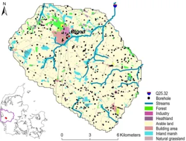
The study area covers a 14.5 km by 13.9 km region located near the town of Ølgod in western Denmark (Fig. 1). This region is dominated by arable land with inland marsh around seven streams. The land surface elevation in this area reaches to about 64 m above mean sea level (a.s.l.) in the northwest-ern part, and decreases to around 17 m a.s.l. in the

southeast-Figure 1. Location and land use of the study area. Black points

denote the 525 boreholes whose logs were used as hard data in the geostatistical simulations.

ern part. The climate is characterized by mean temperatures ranging from 1.4◦C in January to 16.5◦C in August with an annual average around 8.2◦C. Precipitation is highest in autumn and winter while spring is relatively dry, the aver-age annual precipitation is approximately 1050 mm year−1 (Stisen et al., 2011). According to the National Water Re-sources Model (DK-model; Henriksen et al., 2003), the an-nual average groundwater recharge is 611 mm year−1. Wa-ter consumption primarily relies on groundwaWa-ter abstraction. In the Danish national geological JUPITER database (http: //www.geus.dk/jupiter/index-dk.htm), there are 165 pump-ing wells in this area with a total mean abstraction of 3.2×106m3year−1in the period from 2000 to 2010.

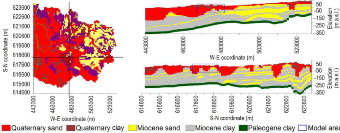
Figure 2 shows the regional geology of the study area as described by Scharling et al. (2009) based on hydrostrati-graphic modelling. This regional-scale model was primar-ily intended to establish the Miocene successions in west-ern Denmark, while less effort was devoted to the modelling of the Quaternary sediments. This model indicates that be-low elevations of−70 m a.s.l., the geology in the study area is dominated by Miocene sediments. Intensive geological mapping in the study area including borehole logs, seismic surveys and airborne transient electromagnetic (SkyTEM) investigations show that the geology at elevations above −70 m a.s.l. is dominated by highly heterogeneous Quater-nary sediments with variable thickness (Høyer et al., 2011). Below, Miocene deposits are located with a thickness of up to about 150 m followed by a Palaeogene clay at the bot-tom (Rasmussen et al., 2010). Accordingly, the geological settings have been conceptualized into five units: Quater-nary sand, QuaterQuater-nary clay, Miocene sand, Miocene clay and Palaeogene clay.

(3)

Figure 2. Regional geological structure, model area in this study is marked with a blue frame. The location is marked by the purple polygon

in Fig. 1, and the horizontal plane is taken at 10 m a.s.l. (modified after Scharling et al., 2009).

Figure 3. Bottom elevation of boreholes in the model area. In

to-tal there are 525 boreholes, but only 22 boreholes are deeper than

−70 m a.s.l.

relatively shallow and only 22 boreholes reach deeper than −70 m a.s.l. (Fig. 3). Therefore, the geological analysis and modelling were performed on Quaternary sediments from the surface down to−70 m a.s.l.

Another important source of information is SkyTEM data (Høyer et al., 2011). The subsurface electrical resistivity data were collected with line spacing from 125 to 270 m, and the soundings penetrated more than 200 m down. The resistivity data have been filtered and inverted using a 19-layer “smooth model”, resulting in a 3-D resistivity data set with cell size of 100 m×100 m×5 m (Høyer et al., 2011). With its high resolution, SkyTEM data are ideal as soft probability data or training image for MPS simulation.

3 Methodology

3.1 Multiple-point geostatistics

MPS was first presented as a direct algorithm in stochastic simulation by Guardiano and Srivastava (1993). Later, Stre-belle (2002) introduced the SNESIM algorithm which com-bines the flexibility of the pixel-based algorithm and the abil-ity to reproduce crisp shapes of the object-based algorithm.

The critical information of sequential simulation is the con-ditional probability distribution function (cpdf), and in the SNESIM algorithm the cpdf of a random variableS(U)is solved by the following equation:

P (S(U)=Sk|dn)∼= ck(dn)

c (dn)

k=1, . . ., K (1)

whereU denotes an arbitrary location, andkdenotes a cer-tain class of lithology, which can haveKcategories in total. dndenotes the data event withndata points included and is obtained by scanning the TI with a search template consisting ofn+1 nodes centred at locationU.c (dn)denotes the num-ber of replicates of a certain conditioning data eventdn, and ck(dn)denotes the number of replicates inc (dn)where the central nodeU has the random variableS(U)=Sk. There-fore, Eq. (1) implies that the probability of stateSk to occur at locationU with conditioning data eventdn equals to the proportionck(dn)/c (dn)from a training image. The solution is achieved by scanning a training image. A training image is a conceptual 2-D or 3-D map which depicts the expected structure and pattern of facies (Strebelle, 2002).

In the practice of stochastic simulation, the cpdf is inte-grated with the sequential simulation paradigm (Goovaerts, 1997, p. 376). The hard data is first assigned to the closest grid nodes, and all the unsampled nodes are visited once and only once in a random path. At each unsampled nodeU, the recorded cpdf corresponding to an actually present hard con-ditioning data event is retrieved and used to draw the simu-lated valueS₍U).

(4)

structure, which can be indicated by TI1 (Table 1). The ellip-soid search template has 240 nodes, and the geometry was set to 2000, 2000 and 60 m for maximum, mean and minimum separately, without any rotation or affinity.

3.2 Soft data conditioning

Soft data or secondary data provide indirect information on the distribution of geological facies. Typical soft data include geophysical data such as seismic data, spaceborne geodetic observations, and airborne electromagnetic data. To be inte-grated in SNESIM, soft data first have to be converted into facies probability data (Strebelle, 2006). The cpdf based on both hard and soft data,P (A|B,C), where “B” indicates the hard data set and “C” indicates the soft data set, is solved by deriving a Bayesian-based model of integratingP (A|B)and P (A|C)(Journel, 2002). In Bayesian statistical terms,P (A) is the facies global proportion or prior probability. And in this case, the notationP (S(U)=Sk|dn)in Eq. (1) can be simpli-fied asP (A|B).P (A|C)denotes the cpdf derived from soft data. The cpdf integrating both hard and soft data is updated as

P (A|B,C)= a τ

aτ₊_b_∗_cτ ∈[0,1] (2) a=1−P (A)

P (A) (3)

b=1−P (A|B)

P (A|B) (4)

c=1−P (A|C)

P (A|C) . (5)

The parameter τ is used to adjust the contribution from soft information “C”.τ =1 indicates that the two data sets “B” and “C” are independent. For τ =0 soft information is ignored, while for τ >1 the influence of soft data “C” is increased, and it is decreased for τ <1 (Journel, 2002). The sensitivity of parameterτ in SNESIM was analysed by Liu (2006), and the choice of parameter values forτ in this study is based on their results.

3.3 SkyTEM data to soft probability

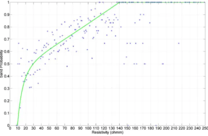
A supervised technique (Liu et al., 2005) was applied to retrieve probabilistic information from SkyTEM data. The resistivity data was converted to facies probability data by correlating the facies occurrence in the borehole lithologi-cal logs with SkyTEM data. The borehole logs were sub-divided into 5 m intervals in correspondence with the dis-cretization of the SkyTEM data. The lithological logs were categorized as sand or clay and the corresponding resistiv-ity value was recorded. Subsequently, for each resistivresistiv-ity bin (size 1·m) the sand probability based on borehole data was computed and plotted against the corresponding resistivity (Fig. 4). The data points were fitted to a truncated polyno-mial non-linear regression function of resistivity (green line).

Figure 4. Non-linear regression of sand occurrence against

SkyTEM data. Blue points are sand occurrence from borehole data compared to resistivity. The green line is the regression function (Eq. 6), coefficient of determination is 0.80 and RMSE is 0.08.

Due to data noise, this least-squares curve fitting was only performed for resistivities between 10 and 140·m. The co-efficient of determination is 0.80 and the root mean square error (RMSE) is 0.08, which indicates that the function rep-resents the correspondence between resistivity (10–140·m) and sand probability satisfactorily. Therefore the polynomial regression model was used to convert the 3-D SkyTEM data (10–140·m) into a 3-D sand probability map. For resistiv-ities lower than 10·m there are only two data points both with sand occurrences of 0, thus sand occurrence was set to 0 below this value. For resistivities higher than 140·m, 80 % of data points show sand occurrence at 1, thus the cor-responding sand occurrence was set to 1. The membership function is therefore expressed as

Ps=      

    

1 if R >140·m

0.0863 ×(lnR)3−0.958×(lnR)2+3.759 ×(lnR)−4.596

if 10·m ≪ R≪ 140·m 0 if R <10·m

(6)

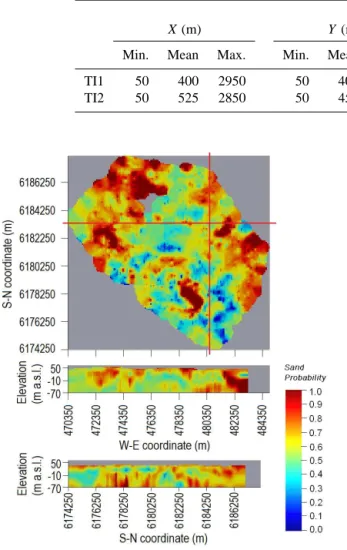
whereR is the resistivity. Figure 5 shows Quaternary sand probability distributions as derived from Eq. (6) for lateral and vertical cross sections.

3.4 Training image

Construction of 3-D TI is challenging since geological pat-terns are usually described in 1-D or 2-D. In this study two kinds of 3-D training images were generated, denoted as TI1 and TI2, respectively.

(5)

Table 1. The mean length distribution inX,Y, andZdirections and proportion of Quaternary clay in TI1 and TI2.

Clay

X(m) Y (m) Z(m)

proportion Min. Mean Max. Min. Mean Max. Min. Mean Max.

TI1 50 400 2950 50 400 3200 2.5 23 60 0.33 TI2 50 525 2850 50 454 3300 2.5 21 65 0.33

Figure 5. Cross sections of the 3-D map showing the probability

of Quaternary sand converted from SkyTEM data. The horizontal plane is taken at 10 m a.s.l.

biased due to the uneven distribution of boreholes. Figure 6 shows the cumulative distribution function (CDF) of resistiv-ity data. The Quaternary clay proportion of 0.33 corresponds to 41.6·m on the CDF curve. Thus, for resistivities be-low this value the sediment is categorized as Quaternary clay, while for resistivities above this value the sediment is cate-gorized as Quaternary sand. Figure 7 (left) illustrates cross sections of TI1.

TI2 was generated by the TiGenerator (Maharaja, 2008), which is a utility package in SGeMS. The TiGenerator (Ma-haraja, 2008) provides a method for generating 3-D train-ing images with parametric shapes ustrain-ing non-iterative, un-conditional Boolean simulation. The user-defined geometry and orientation of simulated objects can be deterministically or statistically described. With the TiGenerator in SGeMS version 2.1, geobodies with sinusoid, ellipsoid, half-ellipsoid and cuboid shapes can be defined by given geometric param-eters such as maximum, median, and minimum radius. The

Figure 6. The CDF of SkyTEM data. Resistivity of 41.6·m cor-responds to a proportion of 0.33, which is the proportion of Quater-nary clay according to borehole data.

geobody is drawn by following a random path until the fa-cies proportion is fulfilled in the simulated grid. The sinusoid shape corresponds to features such as meandering or curvi-linear channels, while the cuboid is rectangular. According to the patterns in TI1, the clay lenses are neither channel-ized nor strongly rectangular, therefore the ellipsoid shape was chosen for the simulation. In TiGenerator the Quater-nary sand was used as background facies and the QuaterQuater-nary clay bodies were simulated with ellipsoid lenses. The target proportion of clay was set to 0.33 as in TI1, and the geomet-ric parameters were determined through the inversion aiming at minimizing the difference between simulated structure and the structure in TI1. The target could also be the information retrieved from borehole data, but in this study the 3-D TI1 de-picts the structure in better detail. Therefore, the information on mean length from TI1 was used in the objective function:

R= v u u t

Pj

t=1(E− ˜E) 2

j (7)

(6)

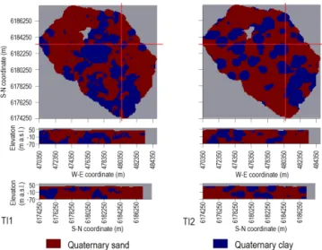
Figure 7. Cross sections of TI1 and TI2. TI1 is converted from

SkyTEM data while TI2 is generated by TiGenerator. The horizon-tal plane is taken at 10 m a.s.l.

Table 1. It shows that both TIs have the same clay proportion and minimum mean length of clay bodies in all directions. While it is difficult and time consuming to match the mean and the maximum length in all three directions, the optimized TI2 has a mean length of 525, 454 and 21 m inX,Y andZ directions, and the corresponding values from TI1 are 400, 400 and 23 m. For the maximum mean length, the difference between TI2 and TI1 is 3 % inXandYdirections, and 8 % in theZdirection, which indicates that the simulated clay body is in the same size range as that from TI1.

Figure 7 (right) shows the cross sections of TI2. Compared to TI1 (Fig. 7, left), the shapes of the clay bodies are more homogeneous and ellipsoidal than the TI1 clay lenses where the size and shape of clay bodies are more heterogeneous. However, the distribution of clay lenses given by TI2 cap-ture the general trends displayed by TI1 fairly well. Both in the horizontal and vertical direction TI2 shows a tendency of clustering, which is also found in TI1.

3.5 Groundwater model

The Groundwater Modelling System (GMS) with the groundwater modelling code MODFLOW-2000 (Harbaugh et al., 2000) was used to assess the effect of the geo-logical structures on the groundwater flow regime, explic-itly on simulated hydraulic head. The model area is char-acterized by high elevations in the central part with sev-eral streams flowing towards the model border, and thus no natural hydraulic boundaries could be identified. Instead, a fixed hydraulic head boundary interpolated from observa-tions was employed. The model bottom is Palaeogene clay which serves as no flow boundary. In order to resemble the finely discretized geological model (100 m×100 m×5 m), the Hydrogeologic-Unit Flow (HUF) package (Evan and

Figure 8. Estimated hydraulic conductivity of Quaternary sand and

Quaternary clay using PEST. The realizations are ranked according to the hydraulic conductivity of the Quaternary sand.

Mary, 2000) was used. The groundwater model was dis-cretized into 63 layers with cells of 100 m×100 m horizon-tally, resulting in a total of 792 603 active cells. A constant layer thickness of 5 m is used from layer 6 to 63, and to avoid dry cells the top layer is 13 m thick on average (in-cluding the unsaturated zone), while the thickness of layer 2 to 5 is 4 m on average. Groundwater recharge from the DK-model (Henriksen et al., 2003) was applied, resulting in an average recharge rate of 611 mm year−1 in the model area. Groundwater discharges to river, drain and abstraction wells, accordingly the RIV (River), DRT (Drain Return) and WEL (Well) packages were enabled in GMS. The nearest stream discharge station is Q25.32, located to the northeast of the model area (Fig. 1). Based on 16-year data (1990– 2005), the average discharge which is scaled to the model area is 59 900 m3d−1. A drain was specified for the entire model area with drain level set to 1 m below terrain, and the drain time constant (1.7×10−2s−1)was taken from the DK-model (Henriksen et al., 2003). There are 165 abstrac-tion wells in the model area with a total pumping rate of 8900 m3d−1 (JUPITER). The groundwater model was cal-ibrated against 219 observations of hydraulic head and the river discharge to station Q25.32 using the inversion code PEST (Doherty, 2005).

(7)

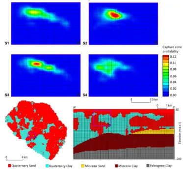
Figure 9. The probabilistic capture zone of Well 1 from each

sce-nario. The well location is illustrated in relation to the geological structure of the TI1.

3.6 Ensemble analysis

To test the effect of the training image and soft condition-ing on geostatistical realizations, multiple-point geostatisti-cal simulations were carried out by applying four different combinations of TIs and soft conditioning (Table 2). The first two scenarios (S1 and S2) were simulated with TI1. Soft conditioning was applied in S2 but not in S1. The other two scenarios (S3 and S4) were simulated with TI2. Soft condi-tioning was applied in S4 but not in S3. According to He et al. (2013) the standard deviation on simulated hydraulic head, based on multiple realizations of the geology, con-verges to a fixed value as more models are accumulated. A stable value is approached after 30 realizations and in this study 50 realizations were therefore generated in each sce-nario and subsequently anchored to the steady state ground-water model.

4 Result and discussion

4.1 Model calibration and groundwater head simulations

With 50 realizations in each scenario, the four scenarios amount to 200 groundwater models. Each model was cali-brated against hydraulic head measurements using the inver-sion code PEST (Doherty, 2005). Initially, a sensitivity

analy-Table 2. Four scenarios of geological realizations used for the

multiple-point geostatistical simulations.

Training Soft Scenario image conditioning

S1 TI1 No

S2 TI1 Yes

S3 TI2 No

S4 TI2 Yes

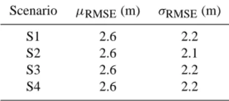
Table 3. RMSE of simulated hydraulic head against observations.

The table lists mean,µRMSE, and standard deviation,σRMSE, over 50 realizations (where each RMSE value is based on 219 observa-tion wells).

Scenario µRMSE(m) σRMSE(m)

S1 2.6 2.2

S2 2.6 2.1

S3 2.6 2.2

S4 2.6 2.2

sis was carried out to identify the parameters to include in the calibration. Based on this analysis the hydraulic conductivi-ties of Quaternary sand, Quaternary clay and Miocene sand were selected as calibration parameters.

The RMSE of simulated hydraulic heads of the calibrated models were used as indicators of model performance. In Ta-ble 3 the mean,µRMSE, and the standard deviation,σRMSE, of the RMSE of the 50 models in each scenario are listed. TheµRMSE is 2.6 m in all four scenarios while theσRMSE is 2.2 m in S1, S3 and S4 and is 2.1 in S2. This implies that models of each scenario are equally well calibrated.

(8)

Table 4. Estimated hydraulic conductivity of Quaternary sand and

Quaternary clay using PEST. The values listed are mean and stan-dard deviationsσ of estimated values over 50 realizations of each scenario (unit: m d−1).

Scenario Quaternary sand Quaternary clay

Mean σ Mean σ

S1 1.7 0.8 0.8 1.1 S2 2.7 0.7 0.4 0.3 S3 1.8 0.4 0.3 0.6 S4 2.9 0.5 0.2 0.2

In addition, the ratio of hydraulic conductivity between sand and clay material is also an indication of the quality of the estimated geological structure where a high contrast would be expected to be the most reasonable result. The mean horizontal hydraulic conductivities of Quaternary sand and clay are listed in Table 4, and it shows that the largest ratio is found for S4 (ratio of 14.5; 2.9–0.2 m d−1), and the second largest ratio is estimated for S2 (ratio of 6.8; 2.7– 0.4 m d−1), while the lowest ratio is found for S1 (ratio of 2.1; 1.7–0.8 m d−1). The difference between the hydraulic con-ductivity of the two units is also visualized in Fig. 8. These results also clearly show the effect of soft data in the simula-tion of geological architecture as the most sound results are obtained for scenarios S2 and S4.

The impact of the training images is seen by comparing the first row (S1 and S2) to the second row (S3 and S4) in

Fig. 8. Scenarios on the first row use TI1 while the scenarios on the second row use the TiGenerator-based TI2. No ap-parent statistical discrepancy can be spotted between these two rows, which means that even though TI2 is not directly derived from field data but from a statistical simulation, the TI2-based realizations yield acceptable results. Both with re-spect to the calibrated groundwater model and the estimated hydraulic parameter values, the choice of training image has a relatively small effect. However, it should be emphasized that TI2 was selected to maximize the similarity between the simulated training image and the field-based training image (TI1), see Table 1.

4.2 Capture zones

(9)

heterogeneity in all the other layers still has a significant con-tribution to the variability of simulated capture zones.

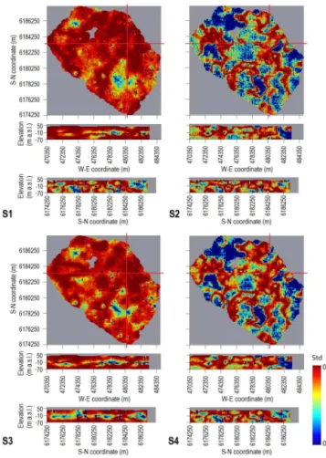
Generally, there is no distinct trend between the first and second row (Figs. 9–11), which again implies that the simu-lation is not sensitive to the differences between TI1 and TI2. For all three wells, the area of the capture zone is smaller for S2 and higher probabilities are found compared to S1. How-ever, this is not the case when comparing S4 to S3. In fact, S3 has a more concentrated probabilistic capture zone than that of S4 for Well 2 and Well 3. In the study of He et al. (2013), the simulation of particle travel time was applied on 100 groundwater models with different geological architecture, in combination with a parameter uncertainty analysis of each model. One discovery was that the geological architecture is the most critical factor regarding particle travel time, because it affects the particle travel path. Therefore, the more con-strained the probabilistic capture zone is, the less dispersed the path lines are, which is a result of less variation between the structures of the geological realizations. The results illus-trated in Figs. 9–11 suggest that there is much less variation among the realizations of S2 than those of S1. This is also in-dicated by the standard deviation of estimated hydraulic con-ductivity (Table 4), where the uncertainty of S2 is smaller than that of S1, especially for the hydraulic conductivity of sand. However, such tendency is not seen in simulations us-ing TI2 (S3 and S4). Apparently the soft conditionus-ing results in less variation between the realizations, and it decreases more in the TI1-based simulations than in TI2-based simula-tions. This is also supported by Fig. 12, where the standard deviation of the 50 realizations of each scenario is illustrated. The standard deviation is computed from the binary geolog-ical units (0 for Quaternary sand and 1 for Quaternary clay). Red colour indicates regions with higher standard deviation, corresponding to higher variability between the 50 realiza-tions. It is obvious that by conditioning on soft data (S2 and S4), the area with higher variability decreases dramatically. S2 is the scenario with the smallest area of high standard de-viations (red colours) among the four scenarios. The expla-nation for this is data redundancy. Realizations from S2 have been over conditioned and therefore the uncertainty on the probabilistic capture zone has been constrained much more than any of the other scenarios.

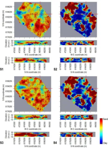
The effect of data redundancy is illustrated in Figs. 13 and 14. Figure 13 shows the E-type map (cell-wise arithmetic av-erage) of each scenario. The “E” stands for “expected value” or precisely “conditional expectation” (Remy et al., 2009, p. 37). On the E-type map the cells are more likely to be sand as the colour turns red, and more likely to become clay as the colour turns blue. The cells with dark red or dark blue colours are cells where hard data (borehole data) are located. The ef-fect of soft data can be seen by comparing Fig. 13 to the soft data (sand probability) in Fig. 5. The E-type of S1 and S3 shows almost no similarity to the soft data in Fig. 5, while the E-type of S2 and S4 show patterns that are very similar to the soft data. Figure 14 illustrates the CDF of soft data

Figure 12. Map of standard deviation over the 50 realizations of

each scenario. The computation of standard deviation is based on binary geological units (0 for Quaternary sand and 1 for Quaternary clay). The standard deviations are 0 at cells where the boreholes are located. The horizontal plane is taken at 10 m a.s.l.

(10)

Figure 13. E-type estimation maps generated from 50 realizations

of the geology of each scenario. The cells where the boreholes are located have the deepest colours. The horizontal plane is taken at 10 m a.s.l.

parameterτis used to adjust the dependence between the two data sets B andC (representing the training image and the soft data in the current case). To make S2 and S4 comparable, the parameterτ is specified to 1.0 in both cases. Liu (2006) pointed out that using a value of 1.0 generates the most ro-bust results. In Fig. 14 the plot for S2 (blue) is lower than the black line in the low probability part, while it is located above the black line in the high probability part, indicating that the S2 realizations are over conditioned. In contrast, as TI2 is remotely related to the soft data, the soft condition-ing on S4 improves the simulations, but the effect of data redundancy is weaker than that in S2. Therefore, integration of the training image constructed using the TiGenerator (TI2) with the SkyTEM-based soft data is more sound than com-bining TI1 and soft data that both are based on SkyTEM data. Journel (2002) found that whenτ <1 the influence of addi-tional data is decreased. Therefore, another scenario (S5) was added where TI1 and soft data were used, but the parameter τ is set to 0.5. S5 corresponds to the green plot in Fig. 14, and it is located right between S1 and S2, which illustrates the effect of decreasingτ.

Figure 14. Black line indicates the CDF of the sand probability

from soft data. Point plots are Q–Q plots of the average of realiza-tions from each scenario against soft data.

5 Conclusions

(11)

obtaining a realistic parameter set is much higher if soft data is used for conditioning. However, when applying soft condi-tioning, the dependence of different data sets has to be taken into account. If the training image and the soft conditioning data are based on the same source of information, the result-ing geological realizations may be over-conditioned. Over-conditioning may not decrease the accuracy of the individ-ual geological model, and this is proved by the calibration where each model from S2 yields reasonable parameter esti-mates. However, over-conditioning decreases the uncertainty among simulated geological models, which results in under-prediction of the uncertainties in transport simulations. This is demonstrated for the examined case where high-resolution SkyTEM data is used as both training image and soft con-ditioning which results in a higher reduction in capture zone uncertainty than if SkyTEM was only used for soft condi-tioning.

Therefore, it is recommended to use independent data sources for generating the training image and the soft data. Based on the present study, the best result is obtained if the TiGenerator is used for defining the training image and the geophysical data for soft conditioning. The information required by the TiGenerator may be derived from expert knowledge of the geological structure of the site or derived from analysis of mapped geology at a site with comparable geology. Alternatively, a Q–Q plot analysis could be carried out and the contribution from soft data on the realization should be decreased. It is, however, (1) problematic to estimate the optimal level of information which should be obtained from the soft data and (2) time consuming to carry out the analysis.

Edited by: A. Guadagnini

References

Bourges, M., Mari, J.-L., and Jeannée, N.: A practical review of geostatistical processing applied to geophysical data: methods and applications, Geophys. Prospect., 60, 400–412, 2012. Carle, S. F. and Fogg, G. E.: Transition probability-based indicator

geostatistics, Math. Geol., 28, 453–76, 1996.

Clement, W. P. and Ward, A.: GPR surveys across a prototype sur-face barrier to determine temporal and spatial variations in soil moisture content, Chap. 23, in: The Handbook of Agricultural Geophysics, edited by: Allred, B. J., Ehsani, M. R., and Daniels, J. J., American Society of Agricultural Engineers, CRC Press, 305–315, 2008.

Comunian, A., Renard, P., Straubhaar, J., and Bayer, P.: Three-dimensional high resolution fluvio-glacial aquifer analog – Part 2: geostatistical modeling, J. Hydrol., 405, 10–23, 2011. Comunian, A., Renard, P., and Straubhaar, J.: 3D multiple-point

statistics simulation using 2D training images, Comput. Geosci. 40, 49–65, 2012.

Coz, M. L., Genthon, P., and Adler, P. M.: Multiple-point statis-tics for modeling facies heterogeneities in a porous medium: the Komadugu-Yobe Alluvium, Lake Chad Basin, Math. Geosci., 43, 861–878, 2011.

Delhomme, J. P.: Spatial variability and uncertainty in groundwater flow parameters: a geostatistical approach, Water Resour. Res., 15, 269–280, 1979.

Deutsch, C. V. and Journel, A. G.: GSLIB Geostatistical Software Library and User’s Guide, Oxford University Press, New York, 1992.

Deutsch, C. V. and Wang, L.: Hierarchical object-based stochastic modeling of fluvial reservoirs, Math. Geol., 28, 857–880, 1996. Doherty, J.: PEST: Model Independent Parameter Estimation, 5th

Edn. of user manual, Watermark Numerical Computing, Bris-bane, Australia, 2005.

Evan, R. A. and Mary, C. H.: Documentation of the hydrogeologic-unit flow (HUF) package, US Geological Survey Open File Rep 00-342, US Geological Survey, Denver, CO, USA, 2000. Goovaerts, P.: Geostatistics for Natural Resources Evaluation,

Ox-ford University Press, New York, 483 pp., 1997.

Guardiano, F. B. and Srivastava, R. M.: Multivariate Geostatistics: Beyond Bivariate Moments, in: Geostatistics Tróia ’92, Quanti-tative Geology and Geostatistics, edited by: Soares, A., Kluwer Academic Publishers, Dordrecht, Netherlands, 133–144, 1993. Harbaugh, A. W., Banta, E. R., Hill, M. C., and McDonald, M. G.:

MODFLOW-2000, the US Geological Survey modular ground-water model – user guide to modularization concepts and the Ground-Water Flow Process: US Geological Survey Open-File Report 00-92, US Department of Interior, Reston, VA, USA, 121 pp., 2000.

Harrar, W. G., Sonnenborg, T. O., and Henriksen, H. J.: Capture zone, travel time, and solute-transport predictions using inverse modeling and different geological models, Hydrogeol. J., 11, 536–548, 2003.

He, X., Sonnenborg, T. O., Jørgensen, F., Høyer, A.-S., Møller, R. R., and Jensen, K. H.: Analyzing the effects of geological and pa-rameter uncertainty on prediction of groundwater head and travel time, Hydrol. Earth Syst. Sci., 17, 3245–3260, doi:10.5194/hess-17-3245-2013, 2013.

Henriksen, H. J., Troldborg, L., Nyegaard, P., Sonnenborg, T. O., Refsgaard, J. C., and Madsen, B.: Methodology for construction, calibration and validation of a national hydrological model for Denmark, J. Hydrol., 280, 52–71, 2003.

Hoffmann, J.: The future of satellite remote sensing in hydrogeol-ogy, Hydrogeol. J., 13, 247–250, 2005.

Hu, L. Y. and Chugunova, T.: Multiple-point geostatistics for mod-eling subsurface heterogeneity: a comprehensive review, Water Resour. Res., 44, W11413, doi:10.1029/2008WR006993, 2008. Huysmans, M. and Dassargues, A.: Application of multiple-point

geostatistics on modeling groundwater flow and transport in a cross-bedded aquifer (Belgium), Hydrogeol. J., 17, 1901–1911, 2009.

Huysmans, M. and Dassargues, A.: Modeling the effect of clay drapes on pumping test response in a cross-bedded aquifer us-ing multiple-point geostatistics, J. Hydrol., 450–451, 159–167, 2012.

(12)

Johnson, N. M.: Characterization of alluvial hydrostratigraphy with indicator semivariograms, Water Resour. Res., 31, 3217–3227, 1995.

Journel, A. G.: Geostatistics: roadblocks and challenges, in: Geo-statistics Tróia ’92, edited by: Soares, A., Springer Netherlands, Dordrecht, 213–224, 1993.

Journel, A. G.: Combining knowledge from diverse sources: an alternative to traditional data independence hypotheses, Math. Geol., 34, 573–596, 2002.

Journel, A. G.: Beyond covariance: the advent of multiple-point geostatistics, in: Geostatistics Banff 2004, Quantitative Geology and Geostatistics, edited by: Leuangthong, O. and Deutsch, C. V., Springer Netherlands, Dordrecht, Netherlands, 225–233, 2005. Klise, K. A., Weissmann, G. S., McKenna, S. A., Nichols,

E. M., Frechette, J. D., Wawrzyniec, T. F., and Tidwell, V. C.: Exploring solute transport and streamline connectivity us-ing lidar-based outcrop images and geostatistical represen-tations of heterogeneity, Water Resour. Res., 45, W05413, doi:10.1029/2008WR007500, 2009.

Liu, Y.: Using the Snesim program for multiple-point statistical sim-ulation, Comput. Geosci., 32, 1544–1563, 2006.

Liu, Y., Harding, A., Abriel, W., and Strebelle, S.: Multiple-point simulation integrating wells, three-dimensional seismic data, and geology, AAPG Bull., 88, 905–921, 2004.

Liu, Y., Harding, A., Gilbert, R., and Journel, A. G.: A work-flow for multiple-point geostatistical simulation, in: Geostatis-tics Banff 2004, Quantitative Geology and GeostatisGeostatis-tics, edited by: Leuangthong, O. and Deutsch, C. V., Springer Netherlands, Dordrecht, Netherlands, 245–254, 2005.

Lubczynski, M. and Roy, J.: Hydrogeological interpretation and po-tential of the new magnetic resonance sounding (MRS) method, J. Hydrol., 283, 19–40, 2003.

Maharaja, A.: TiGenerator: object-based training image generator, Comput. Geosci., 34, 1753–1761, 2008.

Okabe, H. and Blunt, M. J.: Pore space reconstruction using multiple-point statistics, J. Pet. Sci. Eng., 46, 121–137, 2005. Okabe, H. and Blunt, M. J.: Pore space reconstruction of vuggy

carbonates using microtomography and multiple-point statistics, Water Resour. Res., 43, W12S02, doi:10.1029/2006WR005680, 2007.

Pollock, D. W.: User’s guide for MODPATH/MODPATH-PLOT a particle tracking post-processing package for MODFLOW, the US Geological Survey finite-difference ground-water flow model (SuDoc I 19.76:94-464). The Survey Earth Science Information Center, Open-File Reports Section, distributor, 1994.

Rasmussen, E. S., Dybkjær, K., and Piasecki, S.: Lithostratigraphy of the Upper Oligocene – Miocene succession of Denmark, Ge-ological Survey of Denmark and Greenland Bulletin, GeGe-ological Survey of Denmark, Copenhagen, Denmark, 22, 92 pp., 2010. Remy, N., Boucher, A., and Wu, J.: Applied Geostatistics with

SGeMS: A User’s Guide, Cambridge University Press, 2009. Scharling, P. B., Rasmussen, E. S., Sonnenborg, T. O., Engesgaard,

P., and Hinsby, K.: Three-dimensional regional-scale hydrostrati-graphic modeling based on sequence stratihydrostrati-graphic methods: a case study of the Miocene succession in Denmark, Hydrogeol. J., 17, 1913–1933, 2009.

Stisen, S., Sonnenborg, T. O., Højberg, A. L., Troldborg, L., and Refsgaard, J. C.: Evaluation of climate input biases and water balance issues using a coupled surface–subsurface model, Va-dose Zone J., 10, 37–53, 2011.

Strebelle, S.: Conditional simulation of complex geological struc-tures using multiple-point statistics, Math. Geol., 34, 1–21, 2002. Strebelle, S. B.: Sequential simulation for modeling geological structures from training images, in: Stochastic Modeling and Geostatistics: Principles, Methods, and Case Studies, Volume II: AAPG Computer Applications in Geology 5, edited by: Coburn, T. C., Yarus, J. M., and Chambers, R. L., AAPG, Tulsa, OK, USA, 139–149, 2006.

Strebelle, S. B., Payrazyan, K., and Caers, J.: Modeling of a deep-water turbidite reservoir conditional to seismic data using mul-tiple point geostatistics. Society of Petroleum Engineers (SPE) Annual Conference and Technical Meeting, SPE 77429, San An-tonio, TX, 2002.

Sørensen, K. I. and Auken, E.: SkyTEM – a new high-resolution helicopter transient electromagnetic system, Explor. Geophys., 35, 191–199, 2004.