www.atmos-meas-tech.net/8/97/2015/ doi:10.5194/amt-8-97-2015
© Author(s) 2015. CC Attribution 3.0 License.
An evaluation of COSMIC radio occultation data in the lower
atmosphere over the Southern Ocean
L. B. Hande1, S. T. Siems1, M. J. Manton1, and D. H. Lenschow2
1School of Earth, Atmosphere and Environment, ARC Centre of Excellence for Climate System Science, Monash University,
Melbourne, Australia
2National Center for Atmospheric Research, Boulder, Colorado, USA Correspondence to:L. B. Hande (luke.hande@gmail.com)
Received: 18 August 2014 – Published in Atmos. Meas. Tech. Discuss.: 19 September 2014 Revised: 12 December 2014 – Accepted: 15 December 2014 – Published: 9 January 2015
Abstract.The global positioning system (GPS) radio occul-tation (RO) method is a relatively new technique for tak-ing atmospheric measurements for use in both weather and climate studies. As such, this technique needs to be evalu-ated for all parts of the globe. Here, we present an exten-sive evaluation of the performance of the Constellation Ob-serving System for Meteorology, Ionosphere, and Climate (COSMIC) GPS RO observations of the Southern Ocean boundary layer. The two COSMIC products used here are the “wetPrf” product, which is based on 1-D variational analy-sis with European Centre for Medium-Range Weather Fore-casts (ECMWF), and the “atmPrf” product, which contains the raw measurements from COSMIC. A direct comparison of temporally and spatially co-located COSMIC profiles and high resolution radiosonde profiles from Macquarie Island (54.62◦S, 158.85◦E) highlights weaknesses in the ability of both COSMIC products to identify the boundary layer struc-ture, as identified by break points in the refractivity profile. In terms of reproducing the temperature and moisture profile in the lowest 2.5 km, the “wetPrf” COSMIC product does not perform as well as an analysis product from the ECMWF. A further statistical analysis is performed on a large number of COSMIC profiles in a region surrounding Macquarie Island. This indicates that, statistically, COSMIC performs well at capturing the heights of main and secondary break points. However, the frequency of break points detected is lower than the radiosonde profiles suggest, but this could be simply due to the long horizontal averaging in the COSMIC mea-surements. There is also a weak seasonal cycle in the bound-ary layer height similar to that observed in the radiosonde data, providing some confidence in the ability of COSMIC to detect an important boundary layer variable.
1 Introduction
The structure and dynamics of the atmospheric boundary layer (ABL) not only directly impact the weather, through the transport of scalars such as water vapour, but also the climate, most obviously through their role in the formation and dis-sipation of clouds. The ABL height is an important variable, which is controlled by a balance of large-scale subsidence tending to decrease the ABL height and turbulent processes tending to increase the ABL height (Stull, 1988). The exact definition of the ABL height is ambiguous, making it difficult to quantify and study, particularly as routine observations of the depth of the boundary layer are generally not available over much of the globe. This problem is exacerbated over remote locations, such as the Southern Ocean, where in situ observations are sparse. Given that clouds over the Southern Ocean is responsible for large biases in modelled net radi-ation (Trenberth and Fasullo, 2010), it is important to un-derstand the fundamental processes at work in this region, which is dominated by the presence of boundary layer cloud year round (Huang et al., 2012a).
lay-ers in the lowest few kilometres, and these features are not well captured in a state-of-the-art reanalysis data set from the ECMWF. It was shown that the reanalysis data set had a median primary inversion about 200 m lower than the ra-diosonde data. An analysis of proxy cloud fields from the radiosondes indicated that the low-level clouds are not typi-cally capping a well-mixed boundary layer, in stark contrast to the well-studied subtropical stratocumulus in the Eastern Pacific and Atlantic (e.g. Albrecht et al., 1995; Bretherton et al., 2004). Furthermore, multiple cloud layers were ob-served to exist both within, and above the ABL. This sup-ports earlier field observations of boundary layer decoupling in regions with less subsidence as typified in the First Aerosol Characterization Experiment (ACE-1) (Boers and Krummel, 1998; Russell et al., 1998). During ACE-1, as well as the Southern Ocean Cloud Experiments (SOCEX) (Jensen et al., 2000), a main inversion in virtual potential temperature was observed below 2 km from aircraft data, with a weaker inver-sion below the main inverinver-sion. Cloud was observed through-out this decoupled boundary layer.
Another distinctive feature of the Southern Ocean is high wind speeds and wind shear (Hande et al., 2012b; Xiaojun, 2004), producing some of the largest observed wave heights on the globe (Vinoth and Young, 2011). These conditions lead to the possibility of significant sea spray being injected into the boundary layer. This could have an, as yet, unac-counted for effect on the thermodynamics of the boundary layer, as well as the cloud microphysics (Andreas, 1998). With observations supporting an increase in the strength of the Southern Hemisphere westerlies over recent decades (Young et al., 2011; Hande et al., 2012a), the potential long-term impact of these effects on the Southern Ocean boundary layer, as well as the associated clouds, could be significant.
Sokolovskiy et al. (2006) demonstrated the usefulness of using global positioning system (GPS) radio occultation (RO) data to study the ABL height. They found that es-timating the ABL height from the refractivity profile pro-vided good agreement with radiosonde and reanalysis data sets. Most commonly used methods for determining the ABL height from GPS RO data involve identifying large gradients in the refractivity profile (Ao et al., 2012; Basha and Ratnam, 2009). A global analysis of ABL heights was performed by Guo et al. (2011) from GPS RO data. Their technique in-volved looking for a break point, or first-order discontinu-ities, in the refractivity profile, which served as an indicator of the ABL top. It was shown to agree well with boundary layer heights estimated from high-resolution radiosonde ob-servations, particularly in the subtropical high-pressure re-gions where there is often a well-defined decrease in mois-ture above the main inversion. Chan and Wood (2013) use a similar technique to study the global variability of the ABL height. The authors find good agreement of ABL heights be-tween COSMIC and radiosonde data on seasonal timescales. Similarly, Seidel et al. (2010) present a climatology of ABL heights using several methods to estimate the heights
from a number of different measurement systems. That study concludes that ABL heights based on the profile of refractiv-ity do not agree with those based on gradients of other me-teorological variables, particularly in the presence of clouds. There are large differences between different methods to cal-culate the PBL top in the presence of clouds, due to large humidity lapses over cloud top which can commonly lead to higher PBL heights when calculated from the humidity gra-dient. This conclusion is quite poignant, particularly for a cloud-dominated region such as the Southern Ocean.
The aim of this study is to evaluate the performance of the GPS RO technique of measuring boundary layer height, and other significant inversions, as well as the ability of the “wetPrf” COSMIC product to reproduce the temperature and moisture profiles within the boundary layer. An evaluation of this COSMIC data product is needed in this region be-cause the structure of the boundary layer is unlike that of the tropical and subtropical high-pressure region, where the break point method for determining the ABL height has been shown to perform well.
2 Observational and analysis data 2.1 COSMIC
The Constellation Observing System for Meteorology, Ionosphere, and Climate (COSMIC)/Formosa Satellite 3 (FORMOSAT-3) is a constellation of six identical mi-crosatellites each carrying a GPS RO receiver (Anthes et al., 2008). This allows for around 1500–2000 soundings per day around the globe, from 2006 onwards. The COSMIC measurement process is outlined by Kursinski et al. (1997), and summarized below. The primary measurement is of the Doppler shift of a radio signal that is emitted from the GPS satellite, occulted by Earth’s atmosphere, and received by the Low Earth Orbiting satellite on the opposite side of the at-mospheric limb. From this, a bending angle is derived, then the refractivity can be computed as a vertical integral of the bending angle from the top of the atmosphere down. The limb scanning geometry, either rising or setting occultations, is produced by the relative motion of the two satellites.
The raw measurements of the refractivity are used to iden-tify the ABL height using the common technique of identi-fying break points in the refractivity profile, to be discussed in Sect. 3. This technique amounts to computing the vertical derivative of the refractive index, essentially reverting back to the bending angle measurement. This “atmPrf” data set contains approximately 802 data points in the lowest 3 km, and will be referred to as the COSMICraw data set, where
In the neutrally charged atmosphere, the refractive index (N) can be related to the pressure (p), temperature (T) and water vapour pressure (e) by
N =77.6p
T +3.73×10
5 e
T2, (1)
whereT is in Kelvin, andpandeare in hPa. With the aid of the hydrostatic equation, Eq. (1) can be used to estimate vapour pressure if temperature is specified, and vice versa. In this study, the “wetPrf” product was also used, which com-bines the raw observations with moisture information from the ECMWF TOGA 2.5 analysis using 1-D variational analy-sis. The ECMWF analysis product is used as a first guess for moisture below 10 km. The resulting profile is interpolated onto 100 m levels to produce the “wetPrf” profiles. There-fore in this data set, information on moisture and tempera-ture is available at the expense of the high vertical resolution available in the raw refractivity measurements. The refractiv-ity used in the “wetPrf” data set is the analysed refractivrefractiv-ity, not the raw measurements. There are, on average, 31 data points in the lowest 3 km of the profiles over the Southern Ocean, and 400 levels available for the whole sounding. For the sake of clarity, this data product will be referred to as the COSMICwet data set. The profiles are constructed from
50 km long horizontal transects which cover the lowest 3 km. Therefore, the profiles from both COSMIC products would represent an average of the conditions over this line. 2.2 ECMWF analysis
The European Centre for Medium-Range Weather Forecasts (ECMWF) has a number of data products providing global coverage of various atmospheric variables. The ECMWF TOGA 2.5 global Upper Air Analysis data set (ECMWF, 1990) is used here to understand the influence of the back-ground data in the 1-D variational data assimilation. The pro-cess of 1-D variational analysis uses the estimates of mois-ture from the ECMWF data to produce the COSMICwet
mea-surements. This analysis data set is not independent of the other data sets considered here. The Macquarie Island ra-diosonde profiles are used in the assimilation process, how-ever their contribution to the reanalysis data is weighted de-pending on the error characteristics of this data set. These er-ror characteristics are determined by comparing these obser-vations to others in this regions, mostly from satellite-based platforms over the Southern Ocean. When there is agreement between the various observations, the radiosonde data re-ceive a higher weighting, and vice versa. These radiosonde data will be used for the evaluation of the thermodynamics for a limited number of cases. In addition to the radiosonde data, the ECMWF also assimilates the GPS RO data used in this study. Atmospheric profiles from ECMWF represent box-averaged quantities. Thus, these profiles represent the re-gional conditions over a larger portion of the ocean than the radiosonde profiles.
Figure 1.MSLP chart for 2 May 2007 at 12 Z. The approximate location of Macquarie Island is shown by the red dot. (Source: Aus-tralian Bureau of Meteorology.)
2.3 Macquarie Island
Macquarie Island, located at 54.62◦S, 158.85◦E, is one of the few Southern Ocean islands with a dedicated meteoro-logical station. Here, radiosondes are released twice daily from an altitude of 8 m, with direct exposure to the prevailing westerly winds. The data set used here (MAC) consists of the 10 s vertical resolution soundings covering the period 1995– 2014, consisting of 13 396 soundings. On average, there are 171 measurements in the lowest 3 km of the atmosphere. The profiles from the radiosonde represent a point measurement, and as such would be much more representative of the local conditions around Macquarie Island, rather than the regional conditions in the Southern Ocean. The difference in measure-ment techniques between the three data sets will contribute to differences in their respective representations of the atmo-spheric conditions.
The lack of observations at these high latitudes compared to other regions with better coverage of observations reduces the accuracy of numerical weather prediction (Adams, 1997). As a result, the location and extent of cold fronts, for exam-ple, can be inaccurate. The frequency of fronts passing over Cape Grim, Tasmania, was determined by Jimi et al. (1997) to be up to twice a week.
3 Determining the ABL depth
A method for determining the height of the atmospheric boundary layer similar to Guo et al. (2011) is implemented for this study, and outlined below. We look for a break point in the N (z)profile between 100 and 2500 m by defining an approximately 300 m sliding window and calculating the gra-dient of a linear regression of the formAz+Bwithin the win-dow. The break point, which we use as an estimate of ABL height, is defined as the maximum difference ofAfrom the windows immediately above and below the break point. A minimum value of 50 km−1for the gradient of the window immediately below the break point of the main inversion is required. A detailed description of the method is outlined in Guo et al. (2011), including an example of how the method identifies inversions in sounding profiles. A secondary break point, or inversion, is defined in the same way, with a maxi-mum height of 80 % of the height of the main inversion, and a minimum value of 40 km−1for the gradient of the linear gression immediately below the secondary inversion. The re-quirement for having a weaker inversion below a main inver-sion ensures consistency with previous observations of the Southern Ocean boundary layer (Russell et al., 1998; Jensen et al., 2000), and is also commonly observed in other marine environments (Rémillard et al., 2012).
The magnitude of the gradient defining the secondary in-version is weaker than the main inin-version, and hence differs from Guo et al. (2011). This value was chosen so the mean and standard deviation for the height of the secondary in-versions, and also the frequency of occurrence for the MAC data set, were roughly the same as Hande et al. (2012b), who defined the ABL height based on the virtual potential temperature profile from soundings. Changing the value of the gradient below the break point by±5 km−1had little ef-fect on the height of inversions, with changes less than 15 m, but changed the frequency of occurrence by approximately ±16 % for secondary inversions.
The above method for determining the ABL height relies on identifying changes in the refractivity profile. However, it is changes in the temperature and moisture which are often used to define the top of the ABL. So at this point it is worth-while considering how changes in the refractivity relate to changes in temperature and moisture. Differentiating Eq. (1) with height gives
dN dz =77.6
1 T
dp dz−77.6
p T2
dT
dz +3.73×10
5 1
T2
de dz −7.46×10⁵ e
T3
dT
dz. (2)
This shows that gradients inN (z)are linked to gradients in temperature and vapour pressure, which are of the opposite sign. Therefore, the break point technique is most sensitive to a temperature increase and a moisture decrease occurring together. This is typical of a sub-tropical marine boundary layer. However, Hande et al. (2012b) showed that this
struc-ture only occurs in around 18 % of radiosonde data analysed over the Southern Ocean. Both temperature and vapour pres-sure can increase above the ABL, and in this case the refrac-tivity may not necessarily change across the ABL top, and hence no ABL top detected. This was confirmed by tests on idealized profiles which were constructed from a series of straight-line segments with either a temperature or moisture increase or decrease inserted into the profile within the lowest 2 km. The break point method in the refractivity profile often failed to detect an ABL top in the presence of an increase in vapour pressure, even if this occurred at the same level as a strong temperature increase. Obviously this depends on the magnitude of the changes in temperature and moisture; how-ever, the respective magnitudes were chosen to be consistent with observations from MAC.
Chan and Wood (2013) show that the changes in moisture contribute about an order of magnitude more than changes in temperature to the refractivity profile. This has the poten-tial to complicate the ABL top detection over the Southern Ocean, where multiple cloud layers are common, meaning that multiple significant gradients in moisture may be present in the lowest few kilometres.
4 Case study evaluation of COSMIC 4.1 Boundary layer height
Here we use the MAC data set to make a direct comparison with spatially and temporally co-located profiles from COS-MIC to evaluate the performance of the RO technique over the Southern Ocean. COSMIC profiles from within a 2×2 degree box around Macquarie Island occurring within±1 h of the radiosonde launches were considered to be co-located. In addition to this, the COSMIC soundings were required to penetrate to within 500 m of the surface. For the period 2006–2013, only 35 soundings were found to coincide. The small sample is a result of three constraints: the time win-dow, the size of the box, and the requirement to penetrate to below 500 m. Relaxing these constraints makes the sample bigger, but less relevant to the local conditions around Mac-quarie Island. The conclusions presented in this evaluation were drawn from the analysis of all the co-located profiles. However, to emphasize the typical ABL structures encoun-tered over the Southern Ocean, only the results from four profiles will be shown. These four examples are shown in Figs. 2 to 5.
oc-Figure 2.Profiles for 2 May 2007 at 11 Z for MAC (black), COSMICwet(red), COSMICraw(blue), and ECMWF (green). Vertical dashed (dash-dotted) line represents the threshold defining main (secondary) break point.
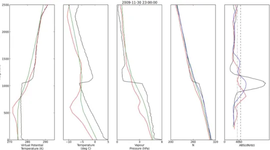
Figure 3.Profiles for 30 November 2009 at 23 Z for MAC (black), COSMICwet(red), COSMICraw(blue), and ECMWF (green). Vertical dashed (dash-dotted) line represents the threshold defining main (secondary) break point.
curring at the same height. The MSLP chart corresponding to Fig. 3 shows that Macquarie Island is under the influence of a high-pressure system, centred just south of Tasmania. There is a sharp drop in the relative humidity just over 1000 m, in-dicating a well-defined cloud top at the same height. This structure represents a typical boundary layer, not unlike those found in the sub-tropics where the break-point method on the refractivity profile has been found to work well (Guo et al., 2011). Finally, Fig. 5 shows no distinctive features, and a more-or-less stably stratified layer extending from about 500 m to above 2.5 km. This final profile is also under the influence of a high-pressure system to the north which pro-duces westerly surface winds. In all the profiles, the black
lines represent the MAC profile, the red is the COSMICwet
product, the green is the background ECMWF analysis pro-file, and the blue refractivity profile is the raw refractivity measurements from the COSMICrawproduct.
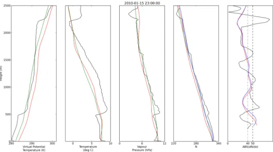
Figure 4.Profiles for 15 January 2010 at 23 Z for MAC (black), COSMICwet (red), COSMICraw(blue), and ECMWF (green). Vertical dashed (dash-dotted) line represents the threshold defining main (secondary) break point.
Figure 5.Profiles for 27 October 2010 at 23 Z for MAC (black), COSMICwet(red), COSMICraw(blue), and ECMWF (green). Vertical dashed (dash-dotted) line represents the threshold defining main (secondary) break point.
Figure 2 shows two clear inversions in virtual potential temperature in the MAC data set, however only one break point in the refractivity profile is detected. The vapour pres-sure increases above both temperature inversions at about 500 and 1200 m, so that the vertical change in refractivity is mostly cancelled out by the coincident increases in tem-perature and vapour pressure. The red profile shows that the COSMICwet product has the same qualitative behaviour as
MAC, however it is consistently slightly warmer and more moist. There are no break points detected here. Interestingly, the higher vertical resolution of the COSMICraw product,
shown as the blue refractivity profile, also fails to detect any break points. The final panel shows the absolute magnitude
of the gradient in refractivity within a 300 m window. The dashed line and the dash-dotted line indicate the thresholds for the main and secondary inversion respectively. Gradients in the refractivity of the COSMICwetand COSMICraw
prod-ucts do not agree in this example.
An example of a well-mixed boundary layer is shown in Fig. 3. There is a strong temperature increase and a corre-sponding moisture decrease around 1100 m. This feature is identified by both the break point method, as well as the vir-tual potential temperature gradient method in the MAC data. Here, the break points in the COSMIC profiles show very good agreement with the MAC data set. The COSMICraw
Table 1.Main and secondary inversion heights for MAC and COSMIC using the refractivity profile break point method (N-bp) and thedθvdz method for MAC.
COSMICwetN-bp COSMICrawN-bp MAC N-bp MACdθvdz
Profile Main Sec Main Sec Main Sec Main Sec
Figure 2 – – – – 1909 – 1188 494
Figure 3 907 – 1187 – 1178 – 1069 –
Figure 4 495 – 595 – 2353 1262 499 178
Figure 5 – – – – 663 520 – –
main inversion in the MAC data. However, the gradient in the refractivity is much smaller. The COSMICwetproduct
identi-fies a break point about 200 m lower than the other data sets. Another decoupled boundary layer is shown in Fig. 4. Here the strongest inversion is at 500 m, with a weaker in-version aloft at 2200 m. The higher inin-version is detected by the break point method. However, since there is an increase in both moisture and temperature at 500 m, the break point method fails to detect the lower one. The COSMICwet
prod-uct has a break point in the refractivity profile at 495 m, nicely coinciding with the main inversion in MAC. Similarly, the COSMICraw product identifies a break point at 595 m,
in approximately the same location. Notice that there is a strong gradient in the refractivity profile from MAC around 600–700 m. This is not identified as a break point since the difference in the gradients between adjacent windows is not larger than those associated with the feature around 1200 m. Also notice that the refractivity gradients of the two different COSMIC products agree very well.
According to the MAC profile in Fig. 5, there are no sig-nificant features in either the temperature or vapour pressure. One would expect no break points or virtual temperature in-versions to be detected, which is true for all but the MAC data set. Here there are two break points in the refractivity profile associated with some slight variability in the vapour pressure between about 300 and 700 m.
As a general observation from the 35 co-located profiles, the break point in the refractivity profile from either COS-MIC products rarely aligns with a virtual potential temper-ature inversion from the high-resolution MAC soundings. The COSMICraw product identifies marginally more break
points (16 main and 9 secondary) than the COSMICwet
prod-uct (15 main and 7 secondary), and there appears to be no systematic difference in height between the two COSMIC data products, or the MAC data set. The common method for identifying the ABL top by identifying large gradients in virtual potential temperature would be inappropriate to use on the COSMICwet data. The diagnostic variables from
COSMICwet, such as virtual potential temperature, which are
derived from a combination of the ECMWF analysis and the raw refractivity (which is in turn derived from the bending angle, which is derived from the first-order measurement of a Doppler shift) are not always consistent with in situ
sound-ings. The COSMICwetvariables can sometimes be
unphysi-cal, such as having superadiabatic layers, as shown in Figs. 3 and 5.
4.2 Thermodynamics
Here we present an evaluation of the ability of the COSMICwetproduct and the ECMWF data to reproduce the
temperature and moisture profiles of the MAC soundings. The root mean squared error (RMSE) for temperature and vapour pressure, calculated using the differences between MAC and COSMICwet, and MAC and ECMWF at three
lev-els in the atmosphere are shown in Table 2. In order to reduce interpolation errors of the data sets, the closest level to 500, 1500 and 2500 m were used as the three levels. The RMSE for each co-located profile and each variable is defined as
RMSE= v u u t
3
X
l=1
(MACl−COSMICwet,l)2, (3)
where MAClis the observed variable from the MAC profile
at levell, and COSMICwet,l is the same for the co-located
COSMICwet profile. The RMSEtotalfor each variable is just
the root mean squared error of each co-located RMSE for that variable. That is,
RMSEtotal=
v u u t
35
X
p=1
RMSE2p, (4)
where RMSEpis the RMSE for each co-located profile.
The quantitative analysis shown in Table 2 indicates that overall, the COSMICwetproduct is poorer than the ECMWF
data at reproducing the MAC temperature and vapour pres-sure. Out of the four profiles shown earlier, only the temper-ature in Fig. 4 and the vapour pressure in Figs. 2 and 5 from COSMICwet perform better than ECMWF. Over the 35
co-located profiles, the ECMWF data outperform COSMICwet
for temperature and vapour pressure, showing the lowest RMSEtotal for both these variables. This is likely due to the
fact that the MAC soundings have been assimilated into the ECMWF data set used here.
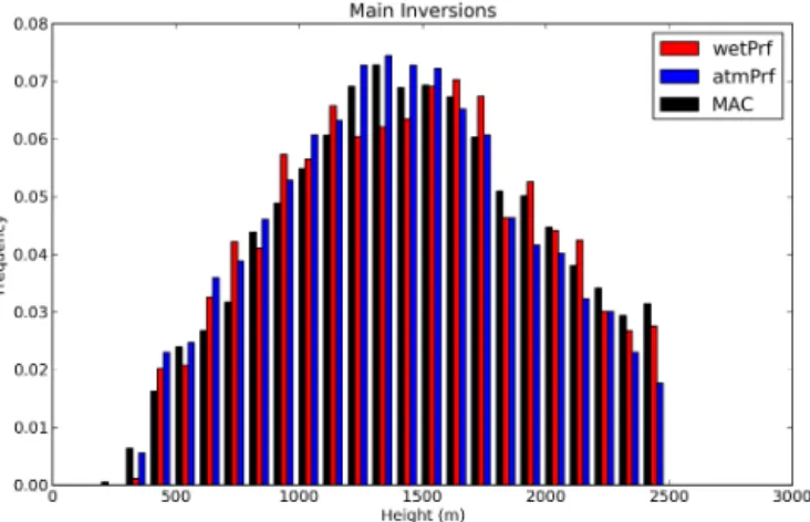
tempera-Figure 6. Main refractivity break point for MAC (black), COSMICwet(red), COSMICraw(blue).
ture inversions which would typically define the ABL top. The COSMICwet product shows the same behaviour as the
background ECMWF data. COSMICwetdoes appear to have
slightly more variability in most of the 35 co-located profiles, however it often produces unphysical superadiabatic layers – for example, in Figs. 3 and 5. Figure 2 is interesting in that the COSMICwetprofile appears to show the same features in
the virtual potential temperature as the MAC data, only off-set by several degrees. This raises the possibility that, given a higher resolution, and more accurate representation of ei-ther the temperature or moisture for the 1D-Var process, the performance of the COSMICwetdata in reproducing the
ther-modynamics and ABL height could be improved.
Schreiner et al. (2007) identify horizontal heterogeneity as a potential source of error in the GPS RO profiles in the neu-trally charged atmosphere. In order to estimate this effect, we consider the impact of a front on the results. An approximate distance to the nearest front, based on MSLP charts, is given in Table 2. The distance to the nearest front is given in 5 de-gree increments in order to reflect the inherent uncertainty in the precise location of the frontal system. Figure 1 is the MSLP chart for the profile shown in Fig. 2, and shows Mac-quarie Island under the influence of a northerly pre-frontal air mass.
There does appear to be a relationship between the perfor-mance of COSMICwet in reproducing the thermodynamics,
and the structure of the ABL, as well as a weak relation-ship to the synoptic meteorology. Analysis of the four best and four worst performing COSMICwetprofiles, as judged by
the RMSE, showed that the best performance of COSMICwet
in reproducing the thermodynamics occurred when the pro-file was stably stratified with no, or only weak inversions and little variability in the profile. These four profiles were typically closer to a cold front, suggesting that the influ-ence of a front is to produce a stably stratified ABL with no strong inversions. On the other hand, the four worst per-forming profiles in reproducing the moisture and
tempera-Figure 7. Secondary refractivity break point for MAC (black), COSMICwet(red), COSMICraw(blue).
ture mostly represented well-mixed ABLs of between 500 and 1200 m depth, with strong temperature inversions and a decrease in vapour pressure occurring together. Figure 3 is one of the four worst performing profiles, which shows a well-defined temperature inversion along with a decrease in moisture around 1000 m. These profiles with strong inver-sions tended to be further away from a front. Hande et al. (2012b) showed that reanalysis products typically have dif-ficulty capturing strong changes in temperature or moisture near Macquarie Island. Hence, a possible explanation for this is the difficulty of the background ECMWF data to identify large gradients in temperature or moisture, and the influence this has on the COSMICwetproduct.
5 Local statistical evaluation
To gain a broader appreciation of the performance of both the COSMIC products, we present a statistical analysis of the height and occurrence of main and secondary inversions. COSMIC RO data from a 10×10 degree box around Mac-quarie Island are used, in order to gain a good statistical sample size. In total, this amounts to 7768 profiles for the COSMICwetproduct, and 7469 for the COSMICrawproduct
over the period 2006–2013. Previous studies (Huang et al., 2012a; Hande et al., 2012b) show that there are only very weak diurnal and seasonal cycles in thermodynamic and cloud properties over the Southern Ocean. Hence, any differ-ence in the temporal distribution of the two data sets should not affect the statistics. Figures 6 and 7 show the distribu-tion of main inversions and secondary inversions from both COSMIC products and MAC.
A main inversion was detected in 3559 of the COSMICwet
soundings, and a secondary inversion in 2002 cases. For the COSMICrawproduct, a main inversion was detected in 3622
sound-Table 2.Root mean squared error for COSMICwetand ECMWF data sets for the temperature (Temp) and vapour pressure (VPres). The approximate distance to a front is also shown in degrees. The letter indicates whether the front is to the west (W) or east (E) of Macquarie Island. The bottom row shows the RMSEtotalfor all the 35 co-located profiles.
COSMICwet ECMWF COSMICwet ECMWF Dist to Temp (◦C) Temp (◦C) VPres (hPa) VPres (hPa) Front (deg)
Figure 2 6.0 2.51 1.05 1.18 10–15 W
Figure 3 7.45 5.06 1.12 0.66 20+ W
Figure 4 3.15 4.11 1.63 1.05 20+ W
Figure 5 6.07 4.26 1.3 1.35 5–10 E
RMSEtotal 27.37 18.5 9.89 8.56
ings. The statistics for the main and secondary break points are shown in Table 3.
From Table 3, it can be seen that the relative frequency of the heights of the inversions are well represented in both COSMIC data sets. This can also be seen in Figs. 6 and 7, where the distribution of the inversions is very similar be-tween the three data sets. The COSMICwetproduct tends to
have slightly higher and less frequent main and secondary break points than the COSMICrawproduct; however, the
dif-ference between the two COSMIC products is small. There is an anomalously high frequency of secondary inversions be-low 500 m in the COSMICwetdata which is often associated
with large gradients in moisture near the surface. Accord-ing to Table 3, the frequency of occurrence of the two break points is significantly less in both COSMIC products com-pared to MAC. Therefore, the difference in vertical resolu-tion between the two COSMIC products does not influence the frequency of main and secondary break points signifi-cantly. The statistics for the MAC data set are close to that of (Hande et al., 2012b), who use the gradient in virtual po-tential temperature to define the inversion heights. This im-plies that, statistically, the method of attributing break points in the refractivity profile to ABL interfaces is appropriate. However, there are intrinsic uncertainties in the measurement of the refractivity profile from the COSMIC products, for example the superadiabatic layers mentioned in the previ-ous section. In terms of representing the height of the ABL, both COSMIC products offer an improvement over a high-resolution reanalysis product from the ECMWF, which was found to underestimate the height of virtual potential temper-ature inversions by about 200 m (Hande et al., 2012b). Note that the ECMWF product is not included here because the vertical resolution is too coarse to reliably compute break points.
We also investigated seasonal and diurnal cycles in the height of main and secondary break points; the statistics are presented in Fig. 8. It is encouraging to note that there is a weak seasonal cycle in the heights of the break points from all data sets, with slightly higher interfaces in South-ern Hemisphere summer than winter. The cycle is less no-table in the secondary break points. December is a nono-table
Table 3.Statistics for the main and secondary break point in the re-fractivity profile for the MAC, COSMICwetand COSMICraw prod-ucts.
MAC COSMICwet COSMICraw Main break point
Frequency (%) 66.7 45.8 48.5
Mean height (m) 1481 1469 1430
Median height (m) 1471 1482 1413
Standard deviation (m) 521 502 517
Secondary break point
Frequency (%) 38.3 25.7 29.6
Mean height (m) 821 809 795
Median height (m) 750 784 733
Standard deviation (m) 349 312 308
Figure 8.Seasonal cycle of main (top) and secondary (bottom) break points for MAC (black), COSMICwet(red), and COSMICraw (blue).
6 Conclusions
The performance of the GPS RO technique of estimating boundary layer heights over the Southern Ocean has been evaluated. A direct comparison between co-located COS-MIC RO soundings and high resolution radiosonde profiles from Macquarie Island show that both COSMIC data prod-ucts identify fewer boundary layer interfaces, identified as break points in the refractivity profile. The method of iden-tifying break points in the refractivity profile as the ABL top has merit. The tests on idealized profiles indicated that this method can reliably identify increases in temperature and/or decreases in moisture, but can have difficulties when both temperature and vapour pressure increase across the in-terface. This type of boundary layer structure is common-place over the Southern Ocean. The full analysis of the 35 co-located profiles shows that there are fewer break points detected in both COSMIC products, compared to the MAC data set. However, when co-located profiles from COSMIC and MAC both identify break points, the heights of the break points mostly agree.
The ability of COSMICwet to reproduce the temperature
and moisture profiles within the boundary layer was evalu-ated by comparison with the MAC soundings. It is shown that the COSMICwet product does not agree with the MAC
soundings as well as the background ECMWF data, even though this product is tied to the background ECMWF data. This illustrates the potential problems of deriving ther-modynamic information from COSMIC data. However, the COSMICwet product does show more variability in the
ver-tical profiles, and the ECMWF data often fail to reproduce large temperature or moisture changes. This suggests that, given a more accurate and high-resolution background data set for the 1-D variational data assimilation, in may be pos-sible to improve upon COSMIC data products.
GPS RO profiles from within a 10×10 degree box around Macquarie Island were used to perform a statistical analysis of the ability of COSMIC to reproduce the main and sec-ondary break point heights. This indicates that, statistically, COSMICwetreproduces the heights of break points in the
re-fractivity profile well, as compared to MAC profiles. How-ever, the frequency is much less. This is true for the raw refractivity measurements as well, which have much higher vertical resolution, indicating that the difference in the fre-quency of boundary layer interfaces detected is not due to differences in vertical resolution. The favourable agreement in terms of height is likely due to the break point detection al-gorithm using the vertical gradient of refractivity to identify break points. This essentially reverts back to the change in the bending angle, which is the fundamental COSMIC mea-surement. Differences between the MAC soundings and the COSMIC products should be expected due to differences in the measurement techniques between the different data sets used in this study. The different methods of averaging used to produce each data set would contribute to some of the
differ-ences in the RMSE values presented in the evaluation of the thermodynamics, as well differences in estimating the ABL height and frequency.
Finally, all data sets produce a weak seasonal cycle in the heights of the interfaces, as one would expect, which is grati-fying. The ability of the COSMIC products to reproduce this ABL feature indicates there is some merit in using the break point of the refractivity profile to identify boundary layer in-terfaces. This analysis shows that the COSMIC data prod-uct is most useful when analysed statistically on seasonal, or longer, timescales.
Acknowledgements. The radiosonde data were obtained from the Australian Bureau of Meteorology. COSMIC data and ECMWF data were obtained from the COSMIC Data Analysis and Archive Center (CDAAC). This research was supported by Monash Univer-sity, Australia. The National Center for Atmospheric Research is sponsored by the National Science Foundation.
Edited by: T. F. Hanisco
References
Adams, N.: Model prediction performance over the southern ocean and coastal region around east antarctica, Aust. Meteor. Mag, 46, 287–296, 1997.
Albrecht, B. A., Bretherton, C. S., Johnson, D., Scubert, W. H., and Frisch, A. S.: The atlantic stratocumulus transition experiment– astex, Bull. Amer. Meteorol. Soc., 76, 889–904, 1995.
Andreas, L. E.: A new sea spray generation function for wind speeds up to 32 ms−1, J. Phys. Oceanogr., 28, 2175–2184, 1998. Anthes, R. A., Ector, D., Hunt, D. C., Kuo, Y.-H., Rocken, C.,
Schreiner, W. S., Sokolovskiy, S. V., Syndergaard, S., Wee, T.-K., Zeng, Z., Bernhardt, P. A., Dymond, K. F., Chen, Y., Liu, H., Manning, K., Randel, W. J., Trenberth, K. E., Cucurull, L., Healy, S. B., Ho, S.-P., McCormick, C., Meehan, T. K., Thomp-son, D. C., and Yen, N. L.: The cosmic/formosat-3 mission: Early results, Bull. Am. Meteorol. Soc., 89, 313–333, 2008.
Ao, C., Waliser, D., Chan, S., Li, J., Tian, B., Xie, F., and Man-nucci, A.: Planetary boundary layer heights from gps radio occul-tation refractivity and humidity profiles, J. Geophys. Res., 117, D16117, doi:10.1029/2012JD017598, 2012.
Basha, G. and Ratnam, M. V.: Identification of atmospheric bound-ary layer height over a tropical station using high-resolution ra-diosonde refractivity profiles: Comparison with gps radio occul-tation measurements, J. Geophys. Res.-Atmos., 114, D16101, doi:10.1029/2008JD011692, 2009.
Boers, R. and Krummel, P. B.: Microphysical properties of bound-ary layer clouds over the southern ocean during ace 1, J. Geo-phys. Res.-Atmos., 103, 16651–16663, 1998.
Bretherton, C. S., Uttal, T., Fairall, C. W., Yuter, S. E., Weller, R. A., Baumgardner, D., Comstock, K., Wood, R., and Raga, G. B.: The epic 2001 stratocumulus study, Bull. Am. Meteorol. Soc., 85, 967–978, 2004.
ECMWF: Ecmwf toga 2.5 degree global surface and upper air anal-yses, daily 1985-continuing. Research Data Archive at the Na-tional Center for Atmospheric Research, ComputaNa-tional and In-formation Systems Laboratory, available at: http://rda.ucar.edu/ datasets/ds111.2/ (last access: 15 October 2013), 1990.
Guo, P., Kuo, Y. H., Sokolovskiy, S. V., and Lenschow, D. H.: Es-timating atmospheric boundary layer depth using cosmic radio occulation data, J. Atmos. Sci., 68, 1703–1713, 2011.
Hande, L. B., Siems, S. T., and Manton, M. J.: Observed trends in wind speed over the southern ocean, Geophys. Res. Lett., 39, L11802, doi:10.1029/2012GL051734, 2012a.
Hande, L. B., Siems, S. T., Manton, M. J., and Belusic, D.: Obser-vations of wind shear over the southern ocean, J. Geophys. Res., 117, D12206, doi:10.1029/2012JD017488, 2012b.
Huang, Y., Siems, T., Manton, S. J., Hande, M. B., and Haynes, M. J.: The structure of low altitude clouds over the southern ocean as seen by cloudsat, J. Climate, 25, 2535–2546, 2012a.
Huang, Y., Siems, T., Manton, S. J., Protat, M. A., and Dela-noe, J.: A study on the low-altitude clouds over the southern ocean using the dardar-mask, J. Geophys. Res., 117, D18204, doi:10.1029/2012JD017800, 2012b.
Jensen, J. B., Lee, S., Krummel, P. B., Katzfey, J., and Gogoasa, D.: Precipitation in marine cumulus and stratocumulus. part i: Thermodynamic and dynamic observations of closed cell circulations and cumulus bands, Atmos. Res., 54, 117–155, doi:10.1016/S0169-8095(00)00040-5, 2000.
Jimi, S. I., Gras, J. L., Siems, S. T., and Krummel, P. B.: A short cli-matology of nanoparticles at the cape grim baseline air pollution station, tasmania, Environ. Chem., 4, 301–309, 1997.
Kursinski, E. R., Hajj, G. A., Schofield, J. T., Linfield, R. P., and Hardy, K. R.: Observing earths atmosphere with radio occulta-tion measurements using global posiocculta-tioning system, Geophys. Res. Lett., 102, 23429–23465, 1997.
Rémillard, J., Kollias, P., Luke, E., and Wood, R.: Marine bound-ary layer cloud observations in the azores, J. Climate, 25, 7381– 7398, 2012.
Russell, L. M., Lenschow, D. H., Laursen, K. K., Krummel, P. B., Siems, S. T., Bandy, A. R., Thornton, D. C., and Bates, T. S.: Bidirectional mixing in an ace 1 marine boundary layer over-lain by a second turbulent layer, J. Geophys. Res., 111, 391–426, 1998.
Schreiner, W., Rocken, C., Sokolovskiy, S., Syndergaard, S., and Hunt, D.: Estimates of the precision of gps radio occultations from the cosmic/formosat-3 mission, Geophys. Res. Lett., 34, L04808, doi:10.1029/2006GL027557, 2007.
Seidel, D. J., Ao, C. O., and Li, K.: Estimating climatological plane-tary boundary layer heights from radiosonde observations: Com-parison of methods and uncertainty analysis, J. Geophys. Res.-Atmos., 115, D16113, doi:10.1029/2009JD013680, 2010. Sokolovskiy, S., Kuo, Y. H., Rocken, C., Schreiner, W. S., Hunt, D.,
and Anthes, R. A.: Monitoring the atmospheric boundary layer by gps radio occultation signals recorded in the open-loop mode, Geophys. Res. Lett., 33, L12813, doi:10.1029/2006GL025955, 2006.
Stull, R.: An introduction to boundary layer meteorology, Vol. 13, Springer, 1988.
Trenberth, K. E. and Fasullo, J. T.: Simulation of present-day and twenty-first-century energy budgets of the southern oceans. Jour-nal of Climate, 23, 440–454, 2010.
Vinoth, J. and Young, I. R.: Global estimates of extreme wind speed and wind height, J. Climate, 24, 1647–1665, 2011.
Xiaojun, Y.: High-wind-speed evaluation in the southern ocean, J. Geophys. Res., 119, D13101, doi:10.1029/2003JD004179, 2004. Young, I. R., Zieger, S., and Babanin, A. V.: Global trends in wind