Measuring the Thermal Conductivities of Low Heat Conducting
Disk Samples by Monitoring the Heat Flow
1
José A. Ibáñez-Mengual*
1Ramón Valerdi-Pérez y
1José A. García-Gamuz
1Departamento de Física, Universidad de Murcia, Campus de Espinardo, 30071 Murcia
ABSTRACT
This artic le a ims to establish an e xperimental procedure to measure heat transmission coefficients in low heat conductive materia ls. The newly developed model takes as starting point the application of Fourie r’s la w to a disk sample when a temperature gradient is established between its faces. The power of a heating element is determined as the heat transfer coeffic ient of the proble m disk. Init ia lly, a glass vessel containing water is placed in direct contact with the heating ele ment; then, a problem plastic disk is placed between this ele ment and the glass vessel, treating the set as a composite wa ll. Prior to the above the water equivalent of a ca lorimetric set (vessel + water + accessories) and the therma l conductivity of the vessel must be determined. The therma l conductivity of the problem plastic disk sa mple is obtained for temperatures ranging fro m 30 to 70° C. The results reveal the existence of some type of structural transition for the proble m materia l.
Keywords
:
thermal conductivity; heat flow; plastic materia l.I.
INTRODUCTION
The proble m of heat conduction in solids has been wide ly studied, and many solutions are available for various boundary conditions, forms and dimensions. Measurement of the therma l p roperties of a material is an impo rtant issue since the parameters associated with it are e xtre mely re levant both in the laboratory and in industrial design [1] [2]. The direct measurement of heat transfer has been studied using several techniques, including the use of circula r heat flow discs, thermistors, as well as comparisons and calibrations of heat flu x sensors [3] [4]. The devices and techniques studied include differentia l scanning calorimeters, improved thin film heat transfer gauges, infrared thermography [5] and liquid crystals [6] and several other visualization techniques [7]. The techniques involved are used for direct measurement of the temperature with thin film thermocouples [8], sputtered micro thermocouples, thermo fluorescence [9], thin-foil thermography [10] and fine wire thermocouples for transient measure ment.
Thermal conductivity [11] [12] has been studied for a wide variety of materia ls [13] [14] [15] [16] using various experimental techniques , such as transient plane source, pulsed and therma l quadruples, electrica l resistance thermo metry [17], t ransient and paralle l hot wire techniques, infra red thermography, laser flash, photoacoustics, etc.
The study in this case is directed towards plastic materials. Due to the great variety of new products intended for recycling, the rapid and accurate determination of their therma l properties is of great importance [18] [19] [20] [21] [22]. The aim of the experiments described was to design a modified Lee 's disk method for measuring therma l
conductivities in samples of low heat conducting materia ls. [23] [24] [25] [26].
II.
THEORY
In the case of water (mass m) in a glass vessel placed on a heating element at te mperature c
> a (roo m te mperature ), as in Figure 1, the power
transferred corresponds to the heat gained due to losses from the system, characterized by 1 and 2
coefficients respectively, resulting in the fo llo wing equation,
a
1
c
2 a
1 2
δQ dθ dθ δQ δQ
= mc +k =C = + =-λ θ-θ -λ θ-θ
dt dt dt dt dt
(1) where (Q/dt)1 and (Q/dt)2 are the net power entering the system fro m the heating ele ment and the losses respectively, θ is its temperature,
a
C
mc
k
is the heat capacity of the system (cathe specific heat of water) and k the water equivalent of the same , wh ich corresponds to the heat capacity of the surrounding vessel, as well as of the measuring probe (accessories). Regrouping terms in the above equation gives
1 2
1 c 2 ad
θ
-
λ +λ θ+λ θ +λ θ =C
dt
,Introducing
1 2, and
1 c
2 a, it follows thatd
θ
dθ
dt
C
=-αθ+
= = dt
dt
-αθ C
(2)with β = C-1. Integrating the above equation between the initial te mperature (θa) and the temperature (θ)
reached at the end of a given time t, yie lds
Figure 1. Heating source + water + system
a
θ
a
θ
a
a
-α dθ -αθ
=-α t ln =-α t αθ- = αθ - exp -α t
-αθ -αθ
θ= - -θ exp -α t α α
(3) so that, if the boundary conditions of the system are applied (
t
0
,
a andt
,
f
(final te mpe rature)), eq. (3) can be written as
f f a f f a
θ=θ - θ -θ exp -α t
θ=θ - θ -θ exp -bt
with
b=
α = =
α
λ +λ
1 2C
C
This equation is of the form
θ=c- a exp -bt
, being
1 c 2 a f
1 2 1 c a f a
1 2
λ θ +λ θ
c=
θ = =
α
λ +λ
λ θ -θ
a=
θ -θ =
λ +λ
(4)
fro m where it immed iately fo llo ws
2 f c1 2 f 1 c 2 a
1 a f
θ -θ
λ
λ +λ θ =λ θ +λ θ
=
λ
θ -θ
(5) and
C b=
λ +λ
1 2 (6) The fina l reduced temperature
-
-
f f c a f
andC
C b
. Taking into account eqs. (6) and (5) yie lds an equationsystem, whose resolution provides expressions for the coefficients 1 and 2:
1 f
2 1 f
C
λ =
1+
θ
λ =λ θ
(7)
Equations (7) correspond to the gain and loss coefficients of the system, whose values give the power supplied by the heating element, in accordance with eq. (1). In part icula r, if we consider that a sufficient time interval has passed to reach the steady state (
f), of the net heat transfer is cancelled, so that (Q/dt)= 0 and the power supplied by the heating ele ment is
1 c f 1
δQ
=
λ θ -θ
dt
(8)2.1. Deter minati on of water e qui valent by the mixtures method.
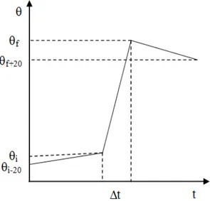
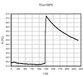
To calculate the power supplied by the heating element, it is necessary to know the water equivalent value of the system k. For this, it is possible to use the mixtu res method; witch consists of introducing a known metal body (copper disk) in the glass vessel containing water at roo m te mperature [27]. The body is previously heated to reach the boiling point of water (100ºC at normal at mospheric pressure). In this way it is possible to know the temperature of the materia l in the water, whose temperature increases. The metal is re moved fro m the water at the end of time interval t and consequently the water temperature decreases due to the cooling effect of its surroundings. Figure 2 outlines the thermogra m corresponding to the full process, which shows three stages: pre-heating, heating and post-heating which, in our case, lasted 20, 1 and 20 minutes, respectively (Figure 3).
TCu=100ºC
t (s)
0 250 500 750 1000 1250 1500 1750 2000 2250 2500
(ºC
)
21.5 22.0 22.5 23.0 23.5 24.0 24.5 25.0 25.5 26.0 26.5 27.0 27.5
Figure 3. Thermogra m fo r the water equiva lent determination. A copper disk o f 43.5 g was used.
The heat balance equation corresponding to the heating stage can be written as
M f i a a f i p
Mc (θ -θ )=(m c +k)(θ -θ )+Q Δt
(9)
where M is the body mass, cM its specific
heats, mais the water mass, cathe water specific heat
capacity, i and f are the init ial and fina l te mperature
corresponding to the heating time interval t, and
p
Q
indicates the losses of heat per unit of time in this stage, which can be estimated as the arithmetic mean of the e xchanges associated to the pre-heating and post-heating stages,
i i-20
pre
p a a
pre post
p p
p
f+20 f
post
p a a
(
θ -θ )
Q =(m c +k)
20
Q +Q
Q =
2
(
θ -θ )
Q
=(m c +k)
20
where
Q
ppre corresponds to therma l stabilization of the glass vessel + water system at temperature
a withθ
i-20 andθ
i are the init ial and final te mperature of this stage andQ
ppost is the heat lost when the metal body is removed and the water te mperature approaches the surrounding temperature,
f andθ
f+20 are the in itia l and final temperatures of the stage.Thus, the energy balance given by equation (9) can be rewritten as
f i-20 f+20 i
M f i a a f i
(θ -θ )+(θ -θ )
Mc (
θ -θ )=(m c +k) (θ -θ )+
40
(10) Equation (10) enables us to determine the water equivalent k value, since we know mass and specific heat capacity of the metal body e mployed.
2.2. Thickness and ther mal conduc ti vity
calculati on for pr oble m materials. Compose d wall method.
When a problem materia l disk samp le, whose heat transmission coeffic ient we wish to know, is placed between a heating source and a glass vessel with wate r, the system corresponds to a composed wall arranged as shown in Figure 4 where k1 and k2
are therma l conductivities and δ1 and δ2thicknesses,
respectively, θi* (i=1,2,3) representstemperatures at
the three interfaces: 1) heating source/sample materia l; 2) sample material/glass layer; 3) g lass layer/water (see Figure 5). The superscript * will be used to indicate that the affected quantities refer to the problem material disk. Given that in the steady state the heat flo w is the same through every ele ment of the composed wall, we can write
* *
* * * * *1 2
* 1 2 3 2
1 2 1 2
1 2 1 2
θ -θ A
θ -θ
θ -θ
δQ
pot
=
=
=
dt
δ
δ
δ
δ
+
k A
k A
k
k
(11) where “pot*” denotes the dissipated power
by the heating source towards the system, A being the common area of different interfaces .
Figure 4. Wall co mposed of two layers: proble m materia l and glass. Profile of te mperature in steady
state.
When the glass vessel with water is placed in d irect contact with the heating source, the power supplied by the source (pot) is given by the expression
2 2 1 1
dQ A
pot =k θ -θ
dt δ
(12)
θ2 being the te mperature at the top of the glass vessel
(at the interface glass/water).
The therma l conductivity of the glass (k2) is
determined fro m equation (12), if the thickness 2 is
known so that it is possible to obtain the therma l conductivity of the problem materia l (k1) fro m
equation (11)
* 1 2 1 * *
1 2 2 2
pot
δ k
k =
θ -θ A k -δ pot
(13)III.
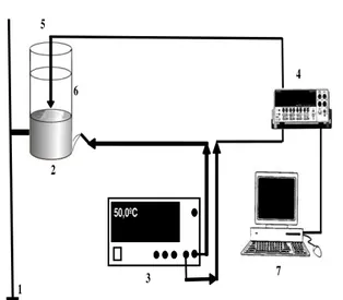
EXPERIMENTAL DEVICE
An e xperimental device was designed, which enables a proble m disk of suitable d imension ( 3 c m, th ickness 2 mm) to be manipulated (see Figure 6). The d isk was placed on top of an alu minu m cylinder of 2 c m th ickness. The cylinder is insulated with armafle x, and an electrical resistance placed within is used as heating ele ment. The heating source temperature c is determined by a type J
thermocouple (iron-constantan, range -210 to 1200 ºC) lodged in the a lu minu m cylinder. The resistance and thermocouple are connected to a control device, provided with a screen that shows instantaneous values of the heating cylinder temperature, c, which
is the parameter that governs and regulates the heating of the system. Another J thermocouple continuously measures the temperature of the deionized water (40 c m3), contained in a g lass vessel (wa ll thic kness 2 mm) placed on of the heating cylinder. This te mperature reaches a final value f for
every c considered. The surface te mperature values
of the heating cylinder (r), for every c value
selected, was determined by means of an infrared thermo meter with configured e missivity (in our case, an Optris® LS thermo meter with infrared dual focus), provided with a laser indicat ion device that directs a beam at the top of the proble m body (shaping a cross oriented to the center of the disk)). This provided a guide for the optimal measuring distance (object distance (D) and foca l measurement area (S), whose D:S ratio in our case is 75:1 for the disk used).
50,0ºC
1 2
3
4
7 5
6
Figure 6. Experimental setup: 1) Support. 2) Heating cylinder with insulating wrapping material. 3) Heat control device. Display with refe rence temperature. 4) Mu ltimete r. 5) Therma l probe in water. 6) Glass
vessel. 7) PC.
IV.
RESULTS AND DISCUSSION
Equation (10) enables the determination of the water equiva lent of our ca lorimetric set k (14,623 g) and consequently the heat capacity, C, whose value (64,623 ca l g-1 ºC-1), together with b in the e xponential fitting (see eq. (4)) for the co rresponding water thermogra m (g lass vessel + water). Figure 7 shows the result obtained for reference te mperature c =50ºC. When te mperature c ranges between 30
and 70ºC (5ºC steps), the coeffic ients 1 and 2 can
be determined (see eq. 7). According to eq. (8), in this case (glass) the power (Q/dt)= 1 (c-f) in eq.
(12) gives the glass heat conductivity k2, knowing the
thickness 2. These results are listed in Table 1.
c=50ºC
t (s)
0 500 1000 1500 2000 2500 3000 3500 4000
(ºC)
21.0 22.0 23.0 24.0 25.0 26.0 27.0 28.0 29.0 30.0 31.0
Figure 7. Thermogra m fo r re ference te mperature c
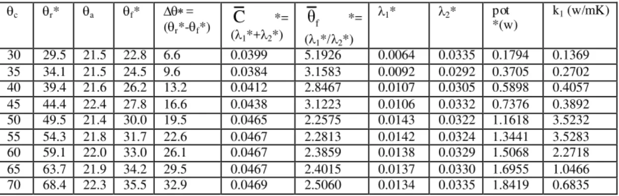
Table 1: Results for the therma l scanning accomplishes in the case of a glass vessel with water placed on the heating cylinder. r is the real te mperature measures with infrared thermo mete r.
Fro m the thermogra ms for the system incorporating the problem materia l disk (PMD) between the heating element and the glass vessel containing water (Figure 5). The values of 1* and
2* were obtained for every te mperature c between
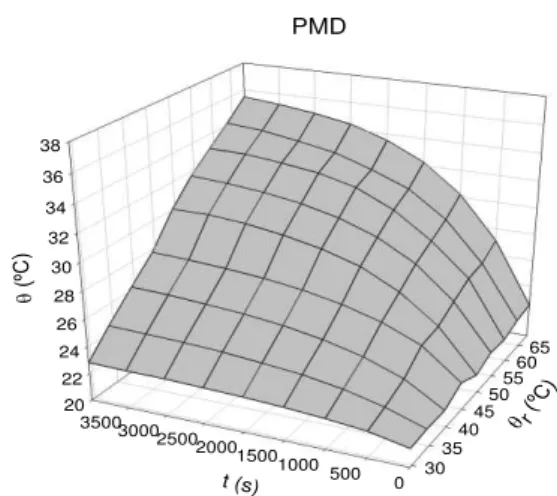
30 and 70ºC (5ºC steps), as well as the heating power (Q/dt)*, whose values permit the determination of the disk thermal conductivity in accordance with (13). Figure 8 shows the corresponding thermogra m at c
= 50ºC and Table 2 lists the results obtained when c
change over the range 30-70 ºC using a PMD placed between the heating cylinder and the glass vessel with water.
c=50ºC
t (s)
0 500 1000 1500 2000 2500 3000 3500 4000
(ºC
)
21.0 22.0 23.0 24.0 25.0 26.0 27.0 28.0 29.0 30.0 31.0
Figure 8. Water te mperature vs. time when c = 50ºC
for the system disk +vessel+water+accesories.
Table 2: Proble m plastic materia l disk: gain and loss parameters (1 and 2), heating power (pot) and heat transmission coefficient (k1) as a function of the measured temperature f.
Figures 9 and 10 depict the meshes corresponding to the thermal behavior of each of the systems (water and PMD). Heating raises the temperature fro m environ mental te mperature (a) to
the final tempe rature (f) corresponding to the steady
state.
20 22 24 26 28 30 32 34 36 38
30 35
40 45
50
5560
65
0 500 1000 1500 2000 2500 3000 3500
(ºC)
r (ºC)
t (s)
Water
Figure 9. Mesh for therma l behavior for the system (glass + water + accessories)
c r a f =(r-f)
C
=(1+2)
θ
f=(1/2) 1 2pot (w) k2
(w/mK) 30 29.5 18.9 23.0 6.5 0.0296 1.6185 0.0113 0.0183 0.3075 0.1028 35 34.1 21.3 25.2 8.9 0.0444 2.3058 0.0134 0.0310 0.5000 0.1222 40 39.4 21.9 27.2 12.2 0.0467 2.3153 0.0141 0.0326 0.7200 0.1283 45 44.4 22.0 28.8 15.6 0.0467 2.3080 0.0141 0.0326 0.9228 0.1286 50 49.5 21.9 30.7 18.8 0.0468 2.1542 0.0148 0.0319 1.1651 0.1350 55 54.3 23.1 32.8 21.5 0.0475 2.2179 0.0148 0.0327 1.3258 0.1344 60 59.1 23.1 34.1 24.9 0.0476 2.2570 0.0146 0.0330 1.5225 0.1330 65 63.7 23.5 35.4 28.3 0.0527 2.3776 0.0156 0.0371 1.8442 0.1420 70 68.4 23.5 36.6 31.7 0.0556 2.4113 0.0163 0.0393 2.1618 0.1483
c r* a f* =
(r*-f*)
C
*=(1*+2*)
f
θ
*=(1*/2*)
1* 2* pot
*(w)
k1 (w/mK)
20 22 24 26 28 30 32 34 36 38
30 35
40 4550
5560 65
0 500 1000 1500 2000 2500 3000 3500
(ºC)
r (ºC)
t (s) PMD
Figure 10. Mesh for thermal behavior for the system (PMD + glass + water + accessories)
Figures 11 and 12 show the values of the heating power and heat transmission coeffic ient corresponding to the glass of the vessel used (system without PMD), while Figures 13 and 14 correspond to the same quantities when PMD is used. In the last case the values obtained for the heat transmission coefficient show a clear peak suggesting out some type of internal structure transition for the PM D between 28 and 34ºC.
Glass
f(ºC)
20 21 22 23 24 25 26 27 28 29 30 31 32 33 34 35 36 37
po
t (w
)
0.00 0.25 0.50 0.75 1.00 1.25 1.50 1.75 2.00 2.25 2.50
Figure 11. Heating power for the system glass +water+accessories vs. te mperature.
Glass
f (ºC)
20 21 22 23 24 25 26 27 28 29 30 31 32 33 34 35 36 37
k 2
(w/
mK)
0.00 0.02 0.04 0.06 0.10 0.12 0.14 0.16 0.18 0.20 0.22
Figure 12. Heat transmission coeffic ients for water
vs. te mperature.
PMD
f
(ºC)
20 21 22 23 24 25 26 27 28 29 30 31 32 33 34 35 36
po
t (w
)
0.0 0.2 0.4 0.6 0.8 1.0 1.2 1.4 1.6 1.8 2.0
Figure 13. Heating power for the co mplete system PMD+g lass+water+accessories vs. temperature.
PMD
f *(ºC)
20 21 22 23 24 25 26 27 28 29 30 31 32 33 34 35 36
k1
(w/mK)
0.0 0.5 1.0 1.5 2.0 2.5 3.0 3.5 4.0
Figure 14. Heat transmission coeffic ients for PMD
vs. te mperature. Note the peak zone at 30-32ºC.
REFERENCES
[1]. A. Hein, N.S. Müller, P.M. Day, V. Kilikoglou, Therma l conductivity of archaeological cera mics: The effect of inclusions, porosity and firing te mperature, Thermochimica Acta 480, 35 (2008). [2]. A. Hein, I. Ka ratasios, N.S. Mülle r, V.
Kilikoglou, Heat transfer properties of pyrotechnical cera mics us ed in ancient meta llurgy, Thermoch imica Acta 573, 87 (2013).
[3]. D. Li, M .A. Wells, Effect of subsurface thermocouple installation on the discrepancy of the measured therma l history and predicted surface heat flu x during a quench operation, Metallurgica l and Materials Transactions B: Process Metallurgy and Materials Processing Science 36 (3), 343 (2005).
[4]. A.V. Murthy, G.T. Fraser, D.P. DeWitt, A summary of heat-flu x sensor calibration data, Journal of Research of the Nat ional Institute of Standards and Technology 110
(2), 97 (2005).
radiant heaters using infrared thermography, NDT and E. International 38 (6), 428 (2005).
[6]. A.D. Ochoa, J.W. Baughn, A.R. Byerley, A new technique for dynamic heat transfer measure ments and flow v isualization using liquid crystal thermography, International Journal of Heat and Fluid Flow 26 (2), 264 (2005).
[7]. J. Fe rnandez-Sea ra et al., Expe rimental apparatus for measuring heat transfer coefficients by the Wilson plot method, European Journal of Physics 26 (3), 1 (2005).
[8]. Y. He ichal, S. Chandra, E. Bordatchev, A fast-response thin film thermocouple to measure rap id surface te mperature changes, Expe rimental Therma l and Fluid Sc ience 30
(2), 153 (2005).
[9]. T.A. Shedd, B.W. Anderson, An automated non-contact wall te mperature measurement using thermoreflectance, Measurement Science and Technology 16 (12), 2483 (2005).
[10]. Y. Liu, X. Zhang, Influence of part icipating med ia on the radiation thermo metry for surface temperature measurement, Journal of Thermal Sc ience 14 (4), 368 (2005). [11]. S. We lze l, H.W. Gronert, E.F. Wassermann,
D.M. Herlach, Influence of the preparation conditions on the thermal conductivity in meta llic glasses , Materials Science and Engineering: A 145 (1), 119 (1991).
[12]. B. Chowdhury, S.C. Moju mda r, Aspects of therma l conductivity relat ive to heat flow, Journal of Therma l Analysis and Ca lorimetry 81 (1), 179 (2005).
[13]. W.N. Dos Santos, Therma l properties of me lt poly me rs by the hot wire technique, Poly mer Testing 24 (7), 932 (2005).
[14]. F. Frusteri et al., Thermal conductivity measure ment of a PCM based storage system containing carbon fibers, Applied Thermal Engineering 25 (11-12), 1623 (2005).
[15]. B. Kshirsagar et al., Therma l contact conductance across gold-coated OFHC copper contacts in different med ia, Journal of Heat Transfer 127 (6), 657 (2005). [16]. B. Re my, A. Deg iovanni, D. Maillet,
Measurement of the in -plane therma l diffusivity of materia ls by infrared thermography, International Journal of Thermophysics 26 (2), 493 (2005).
[17]. M.C. Ga rcia -Payo, M.A. Izquie rdo-Gil, Thermal resistance technique for measuring the therma l conductivity of thin
microporous me mbranes , Journal of Physics D-Applied Physics 37 (21), 3008 (2004). [18]. N. So mbatsompop, A.K. Wood,
Measurement of therma l conductivity of polymers using an improved Lee's Disc apparatus, Poly mer Testing 16 (3), 203 (1997).
[19]. D.M Price, M . Jarratt, Therma l conductivity of PTFE and PTFE co mposites , Thermochimica Acta 392–393, 231 (2002). [20]. A., Nidaa, Effect of Heat Treatment On
Tensile Strength, Ha rdness and Therma l conductivity of Blended Poly me r Co mposite, Proceedings of 7th International Conference on Processing and Manufacturing of Advanced Materials, Quebec City, CANADA, 2012, edited by T. Chandra, M. Ionescu, D. Mantovani, (Ed.), Vo l. 706
(Quebec City, CANA DA, 2012).
[21]. S. Mahesh, S.C. Joshi, Therma l conductivity variations with co mpos ition of gelatin-silica aerogel-sodium dodecyl sulfate with functionalized multi-walled carbon nanotube doping in their co mposites , International Journal o f Heat and Mass Transfer 87, 606 (2015).
[22]. M. Rides, J. Morikawa , L. Ha lldahl, B. Hay, H. Lobo, A. Dawson, C. Allen, Intercomparison of therma l conductivity and therma l d iffusivity methods for plastics , Poly mer Testing 28, 480 (2009).
[23]. N. So mbatsompop, A.K. Wood, Measurement of Thermal Conductivity of Polymers using an Improved Lee’s Disc Apparatus, Polyme r Testing 16, 203 (1997). [24]. O.S. Sa mue l, B.O. Ra mon, Y.O. Johnson,
Thermal Conductivity of Three Different Wood Products of Co mbretaceae Fa mily; Terminalia superb, Terminalia ivorensis and Quisqualis indica, Journal of Natura l Sciences Research 2 (9), 18 (2012).
[25]. M. Ala m, S. Rah man, P.K. Halde r, A. Raquib, M. Hasan, Lee’s and Charlton’s Method for Investigation of Therma l Conductivity of Insulating Materials , Journal of Mechanical and Civil Engineering 3 (1), 53 (2012).
[26]. P. Philip, L. Fagbenle, Design of lee’s disc electrica l method for determining therma l conductivity of a poor conductor in the form of a flat disc, International Journa l of Innovation and Scientific Research 9 (2), 335 (2014).