Statistical Analysis of the Correlation between the Happy Planet Index and the Gross Domestic Product Per Capita, in Romania

Annals of “Dunarea de Jos” University of Galati Fascicle I. Economics and Applied Informatics

Years XXII – no_3/2016

ISSN-L 1584-0409 ISSN-Online 2344-441X

www.eia.feaa.ugal.ro

Statistical Analysis of the Correlation between the

Happy Planet Index and the Gross Domestic Product Per

Capita, in Romania

Gabriela OPAIT

A R T I C L E I N F O A B S T R A C T Article history:

Accepted November Available online December

JEL Classification

C , C , C

Keywords:

(appy Planet )ndex, Gross Domestic Product per capita, Correlation Raport

This paper reflects the architecture of the methodology for to achieve the statistical modeling of the trend concerning the correlation between the (appy Planet )ndex and the Gross Domestic Product per capita in Romania, between - . with the help of the „Least Squares Method . Also, this paper reflects the manner in which we can to measure the intensity of the correlation between the (appy Planet )ndex and the Gross Domestic Product per capita in Romania, between - with the help of the Correlation Raport.

© EA). All rights reserved.

1. Introduction

)n this research, ) present a personal contribution which reflects a statistical analysis of the trend model concerning the correlation between the (appy Planet )ndex and the Gross Domestic Product per capita in Romania, in the period - . The purpose of the research reflects the possibility for to calculate the intensity regarding the correlation between the values of the (appy Planet )ndex and the values of the Gross Domestic Product per capita in Romania, in the period - , by means of the Correlation Raport. The statistical methods used are the „Coefficients of Variation Method , respectively the „Least Squares Method applied for to calculate the parameters of the regression equation. The sections presents the methodology for to achieve the trend model concerning the Gross Domestic Product per capita in Romania, in the period - , with the help of the „Least Squares Method . The section reflects the architecture concerning the modeling of the trend between the values of the Gross Domestic Product per capita and the values of the (appy Planet )ndex between - , concerning Romania. The section presents the research regarding the intensity of the correlation between the values of the Gross Domestic Product per capita in Romania and the values of the (appy Planet )ndex in Romania, in the period - . The state of the art in this domain is represented by the research belongs to Carl Friederich Gauss, who created the „Least Squares Method[ ].

2. The modeling of the trend concerning the Gross Domestic Product per capita in Romania, between 2006-2013

)n the period - , we observe the next evolution regarding the Gross Domestic Product per capita in PCS in Romania, according to the table no. :

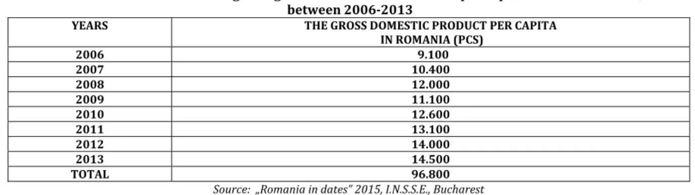
Table no. 1 The evolution regarding the Gross Domestic Product per capita in PCS in Romania, between 2006-2013

YEARS THE GROSS DOMESTIC PRODUCT PER CAPITA IN ROMANIA (PCS)

2006 9.100

2007 10.400 2008 12.000 2009 11.100 2010 12.600 2011 13.100 2012 14.000 2013 14.500 TOTAL 96.800

We want to identify the trend model concerning the Gross Domestic Product per capita in Romania, between the period - , using the table no. .

- if we formulate the null hypothesis

H

0: which mentions the assumption of the existence for the model of

tendency concerning X factor, where X = the Gross Domestic Product per capita in Romania, as being the

function

α

ti

=

a

+

b

⋅

β

i, then the parameters a and b of the adjusted linear function, can to be calculated by

means of the next system [ ]:

∑

∑

= =

=

−

−

=

⇔

=

−

=

n i i i n i ti

i

x

S

x

a

bt

x

S

1 2 1 2

min

)

(

min

)

(

⇒

⎪

⎪

⎩

⎪⎪

⎨

⎧

=

∂

∂

=

∂

∂

0

0

b

S

a

S

⇒

⎪

⎪

⎩

⎪⎪

⎨

⎧

−

=

−

−

−

−

=

−

−

−

∑

∑

= = n i i i n i i

t

bt

a

x

bt

a

x

1 1 1 1

)

2

1

/(

0

)

)(

(

2

)

2

1

/(

0

)

1

)(

(

2

⇒

⎪

⎪

⎩

⎪⎪

⎨

⎧

=

+

=

+

∑

∑

∑

∑

∑

= = = = = n i i i n i i n i i n i i n i i

t

x

t

b

t

a

x

t

b

na

1 1 2 1 1 1 Therefore,

∑

∑

∑

∑

∑

∑

∑

∑

∑

∑

∑

∑

∑

= = = = = = = = = = = = = ⎟ ⎠ ⎞ ⎜ ⎝ ⎛ − − = = n i n i i i n i i n i i n i i i n i i i n i i n i i n i i n i n i i i n i i n i i t t n t t x t x t t t n t t x t x a i 1 2 1 2

1 1 1 1

2 1 2 1 1 1 2 1 1 1 2 1 1 2 1 1 1 1 2 1 1 1 1 1 ⎟ ⎠ ⎞ ⎜ ⎝ ⎛ − − = =

∑

∑

∑

∑

∑

∑

∑

∑

∑

∑

∑

= = = = = = = = = = = n i i n i i n i i n i i n i i i n i n i i n i i n i i i n i i n i i t t n x t t x n t t t n t x t x n b i

Table no. 2 The estimate of the value for the variation coefficient in the case of the adjusted linear function, in the hypothesis of the linear evolution concerning the

Gross Domestic Product per capita in Romania, between 2006-2013

LINEAR TREND

YEARS

THE GROSS DOMESTIC PRODUCT PER CAPITA

IN ROMANIA (PCS)

(xi)

t

i

2 i

t

i i

x

t

i

t

a

bt

x

i

=

+

i

t i x

x ₋

2006 9.100 - - . . , ,

2007 10.400 - - . . , ,

2008 12.000 - - . . , . ,

2009 11.100 - - . . , ,

2010 12.600 . . , ,

2011 13.100 . . , ,

2012 14.000 . . , ,

2013 14.500 . . , ,

TOTAL 96.800 . . ,

)f we calculate the statistical data for to adjust the linear function, we obtain for the parameters a and b the values:

12.100

0 60 8 0 100 . 36 60 800 . 96 2 = − ⋅ ⋅ − ⋅ = a

_601,6666667

0 60 8 800 . 96 0 100 . 36 8 2 = − ⋅ ⋅ − ⋅ = b

100

2

,

69

%

800

.

96

666666

,

606

.

2

100

100

:

⋅

=

⋅

=

−

=

⋅

⎥

⎥

⎥

⎥

⎦

⎤

⎢

⎢

⎢

⎢

⎣

⎡

−

=

∑

∑

∑

∑

− = − = − = − = m m i i m m i I t i m m i i m m i I t i I

x

x

x

n

x

n

x

x

v

i i

- in the situation of the alternative hypothesis

H

1: which specifies the assumption of the existence for the

model of tendency regarding X factor, where X= the Gross Domestic Product per capita in Romania,as being

the quadratic function 2

i i

t

a

b

t

ct

x

i

=

+

⋅

+

, the parameters a, b şi c of the adjusted quadratic function, can to

be calculated by means of the system [ ]:

∑

∑

= =

=

−

−

−

=

⇔

=

−

=

n i i i i n i ti

i

x

S

x

a

bt

ct

x

S

1 2 2 1 2

min

)

(

min

)

(

⇒

⎪

⎪

⎪

⎩

⎪

⎪

⎪

⎨

⎧

=

∂

∂

=

∂

∂

=

∂

∂

0

0

0

c

S

b

S

a

S

⇒

⎪

⎪

⎪

⎪

⎩

⎪⎪

⎪

⎪

⎨

⎧

−

=

−

−

−

−

−

=

−

−

−

−

−

=

−

−

−

−

∑

∑

∑

= =

)

2

1

/(

0

)

)(

(

2

)

2

1

/(

0

)

)(

(

2

)

2

1

/(

0

)

1

)(

(

2

2 2 1 1 2 1 1 2 i i i i n i i i i n i i i

t

ct

bt

a

x

t

ct

bt

a

x

ct

bt

a

x

Therefore,

⎪

⎪

⎪

⎩

⎪

⎪

⎪

⎨

⎧

⋅

=

+

+

⋅

⋅

=

+

⋅

+

=

+

+

⋅

∑

∑

∑

∑

∑

∑

∑

∑

∑

∑

∑

= = = = = = = = = = = n i i i n i i n i i n i i n i i i n i i n i i n i i n i i n i i n i i

x

t

t

c

t

b

t

a

x

t

t

c

t

b

t

a

x

t

c

t

b

a

n

1 2 1 4 1 3 1 2 1 1 3 1 2 1 1 1 2 1

∑

∑

∑

∑

∑

∑

= = = = = =

⎟

⎠

⎞

⎜

⎝

⎛

−

⋅

−

=

n i n i i i n i i n i i i n i i n i i i

t

t

n

x

t

t

x

t

a

1 2 1 2 4 1 1 2 1 2 1 4

∑

∑

= =

=

n i i n i i i

t

t

x

b

1 2 1

∑

∑

∑

∑ ∑

= = = = =

⎟

⎠

⎞

⎜

⎝

⎛

−

⋅

−

⋅

⋅

=

n i n i i i n i n i n i i i i i

t

t

n

x

t

x

t

n

c

1 2 1 2 4

1 1 1

Table no. 3 The estimates of the value for the variation coefficient in the case of the adjusted quadratic function, in the hypothesis of the parabolic evolution regarding the Gross Domestic Product

per capita in Romania, between 2006-2013

PARABOLIC TREND

YEARS

THE GROSS DOMESTIC PRODUCT PER

CAPITA IN ROMANIA

(PCS) (xi)

3

i

t

t

_i4

t

_i2

x

_i

2

i i

t

a

bt

ct

x

i

=

+

+

i

t i x

x ₋

2006 9.100 - . . , ,

2007 10.400 - . . , ,

2008 12.000 - . . , ,

2009 11.100 - . . , ,

2010 12.600 . . , ,

2011 13.100 . . , ,

2012 14.000 . . , ,

2013 14.500 . . , ,

TOTAL 96.800 . . ,

)f we calculate the statistical data for to adjust the quadratic function, we obtain for the parameters a,b and c

the next values:

⇒

⎪

⎩

⎪

⎨

⎧

=

⋅

+

⋅

+

⋅

=

⋅

+

⋅

+

⋅

=

⋅

+

⋅

+

⋅

300

.

721

708

0

60

100

.

36

0

60

0

800

.

96

60

0

8

c

b

a

c

b

a

c

b

a

a

=

12

.

236

,

62791

b

₌

₆₀₁

_,

_6666667

c

₌

₋

₁₈

_,

_21705426

So, the coefficient of variation for the adjusted quadratic function has the value:

%

67

,

2

100

800

.

96

449624

,

588

.

2

100

100

:

⋅

=

⋅

=

−

=

⋅

⎥

⎥

⎥

⎥

⎦

⎤

⎢

⎢

⎢

⎢

⎣

⎡

−

=

∑

∑

∑

∑

− = − = −

= −

=

m

m i

i m

m i

II t i m

m i

i m

m i

II t i

II

x

x

x

n

x

n

x

x

v

i i

- in the case of the alternative hypothesis

H

_{2 : which describes the supposition of the existence for the model}

of tendency concerning X factor, where X = the Gross Domestic Product per capita in Romania,as being the

exponential function i

i

t

t

ab

x

₌

_{, then the parameters a and b of the adjusted exponential function, can to be}

calculated by means of the next system [ ]:

∑

∑

= =

=

−

−

=

⇔

=

−

=

n

i

i i

n

i

t

i

x

S

x

a

t

b

x

S

i

1

2 1

2

min

)

lg

lg

(lg

min

)

lg

(lg

⇒

⎪

⎪

⎩

⎪⎪

⎨

⎧

=

∂

∂

=

∂

∂

0

lg

0

lg

b

S

a

S

⇒

⎪

⎪

⎩

⎪⎪

⎨

⎧

−

=

−

−

−

−

=

−

−

−

∑

∑

= =

n

i i

i n

i i

t

b

t

a

x

b

t

a

x

1 1

1 1

)

2

1

/(

0

)

)(

lg

lg

(lg

2

)

2

1

/(

0

)

1

)(

lg

lg

(lg

2

⎪

⎪

⎩

⎪⎪

⎨

⎧

⋅

=

⋅

+

=

⋅

+

⋅

∑

∑

∑

∑

∑

= =

=

= =

n

i

i i n

i i n

i i

n

i i n

i i

x

t

t

b

t

a

x

t

b

a

n

1 1

2 1

1 1

lg

lg

lg

lg

lg

lg

Thus,

∑

∑

∑

∑

∑

∑

∑

∑

∑

∑

∑

∑

∑

= =

= = = =

= =

= = =

= =

⎟ ⎠ ⎞ ⎜ ⎝ ⎛

− − =

=

n

i

n

i i i

n

i i

n

i i n

i

i i n

i i i

n

i i n

i i

n

i i n

i n

i

i i

n

i i n

i i

t t

n

t x t t

x

t t

t n

t x t

t x

a

i

1

2

1 2

1 1 1 1

2

1 2

1 1

1 2

1

1 1

lg lg

lg lg

lg

and

∑

∑

∑

∑

∑

∑

∑

∑

∑

∑

∑

= =

= = =

= =

= = =

=

⎟ ⎠ ⎞ ⎜ ⎝ ⎛

− − ⋅

= =

n

i

n

i i i

n

i i

n

i i n

i i i

i

n

i i n

i i

n

i i n

i

i n

i i

n

i i

t t

n

t x x

t n

t t

t n

x t t

x n

b

i

1

2

1 2

1 1 1

1 2

1 1 1 1

1

lg lg

lg lg

lg

Table no. 4 The estimate of the value for the variation coefficient in the case of the adjusted exponential function, in the hypothesis concerning the exponential evolution regarding

the Gross Domestic Product per capita in Romania, between 2006-2013

EXPONENTIAL TREND

YEARS

THE GROSS DOMESTIC PRODUCT PER

CAPITA IN ROMANIA

(PCS) (xi)

i

x

lg

t

i

lg

x

i

lg

x

ti

=

b t

a _ilg

lg + =

ti

ti

ab

x

₌

i

t i x

x ₋

2006 9.100 , - , , , ,

2007 10.400 , - , , , ,

2008 12.000 , - , , , ,

2009 11.100 , - , , , ,

2010 12.600 , , , , ,

2011 13.100 , , , , ,

2012 14.000 , , , , ,

2013 14.500 , , , , ,

TOTAL 96.800 , , , ,

Consequently, if we calculate the statistical data for to adjust the exponential function, we obtain for the parameters a and b the values:

4,078214604 8

62571684 ,

32

lga= =

_0,022130303

60 327818195 ,

1

lgb= =

%

73

,

2

100

800

.

96

754667

,

642

.

2

100

100

:

exp exp

exp

⋅

=

⋅

=

−

=

⋅

⎥

⎥

⎥

⎥

⎦

⎤

⎢

⎢

⎢

⎢

⎣

⎡

−

=

∑

∑

∑

∑

− = − = −

= −

=

m

m i

i m

m i

t i m

m i

i m

m i

t i

x

x

x

n

x

n

x

x

v

i i

We apply the coefficients of variation method as criterion of selection for the best model of trend. We notice that:

%

73

,

2

%

69

,

2

%

67

,

2

<

=

<

_exp

=

=

v

v

v

_{II I}

So, the path reflected by X factor, which represents the Gross Domestic Product per capita in Romania, between 2006-2013, is a parabolic trend of the shape

x

t_i

=

a

+

b

⋅

t

i

+

ct

i2, with other words it confirms

the hypothesis

H

1 .

0 10000

2006 2007 2008 2009 2010 2011 2012 2013

THE PARABOLIC TREND CONCERNING THE GROSS DOMESTIC PRODUCT PER CAPITA IN ROMANIA, BETWEEN 2006-2013

The type no. 1 The trend model of the values regarding the Gross Domestic Product per capita in Romania, between 2006-2013

We observe that, the cloud of points which reflects the values concerning the Gross Domestic Product per capita in Romania, between - , it carrying around a quadratic trend model, according to the type no.

.

3. The modeling of the trend between the G.D.P. per capita and the Happy Planet Index between 2006-2013, for Romania

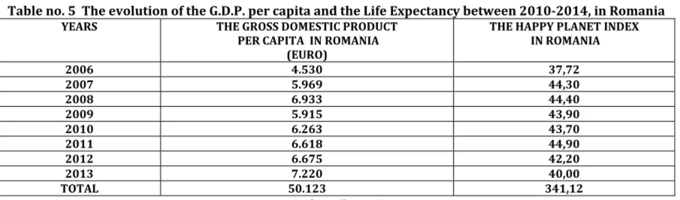
Table no. 5 The evolution of the G.D.P. per capita and the Life Expectancy between 2010-2014, in Romania

YEARS THE GROSS DOMESTIC PRODUCT PER CAPITA IN ROMANIA

(EURO)

THE HAPPY PLANET INDEX IN ROMANIA

2006 4.530 37,72

2007 5.969 44,30

2008 6.933 44,40

2009 5.915 43,90

2010 6.263 43,70

2011 6.618 44,90

2012 6.675 42,20

2013 7.220 40,00

TOTAL 50.123 341,12

Source: „Romania in dates , ).N.S.S.E., Bucharest

We want to identify the trend model between the G.D.P. per capita and the (appy Planet )ndex for Romania, in the period - , using the table no. .

- if we formulate the null hypothesis

H

0: which mentions the assumption of the existence for the model of

tendency concerning

ω

factor, where

ω

= the Happy Planet Index in Romania, as being the function

i

ti

a

b

ξ

ω

=

+

⋅

, then the parameters a and b of the adjusted linear function, can to be calculated by means of

the next system [ ]:

⎪

⎪

⎩

⎪⎪

⎨

⎧

⋅

=

⋅

+

=

+

⋅

∑

∑

∑

∑

∑

= =

=

= =

n

i

i i n

i i n

i i

n

i i n

i i

b

a

b

a

n

1 1

2 1

1 1

ω

ξ

ξ

ξ

ω

ξ

Therefore,

∑

∑

∑

∑

∑

∑

= =

= = =

=

−

−

=

n

i i n

i i

i n

i i n

i i n

i i n

i i

n

a

1 2 1

2

1 1 1

1 2

)

(

ξ

ξ

ω

ξ

ξ

ω

ξ

∑

∑

∑

∑

∑

= =

= = =

−

−

=

n

i i n

i i

n

i i n

i i n

i i i

n

n

b

1 2 1

2

1 1 1

)

(

ξ

ξ

ω

ξ

ω

ξ

Table no. 6 The estimate of the value for the variation coefficient in the case of the adjusted linear function, in the hypothesis concerning the linear evolution of the

correlation between the G.D.P. per capita in Romania and the Happy Planet Index in Romania, between 2006-2013

LINEAR TREND

YEARS

THE G.D.P. PER CAPITA IN ROMANIA (MII EURO)

(

ξ

i)

THE HAPPY PLANET

INDEX IN ROMANIA

(

ω

i)

2

i

ξ

(106₎

i i

ω

ξ

(103₎

i

b

a

i

ξ

ω

_ξ

=

+

i

i

ω

_ξ

ω

−

2006 4,530 37,72 , , , ,

2007 5,969 44,30 , , , ,

2008 6,933 44,40 , , , ,

2009 5,915 43,90 , , , ,

2010 6,262 43,70 , , , ,

2011 6,618 44,90 , , , ,

)f we calculate the statistical data for to adjust the linear function, we obtain for the parameters a and b the

values:

33

,

79933213

)

10

123

,

50

(

10

910693

,

318

8

10

1183

,

144

.

2

10

123

,

50

12

,

341

10

910693

,

318

2 3 6 3 3 6

=

⋅

−

⋅

⋅

⋅

⋅

⋅

−

⋅

⋅

=

a

0

,

001411035

)

10

123

,

50

(

10

910693

,

318

8

12

,

341

10

123

,

50

10

1183

,

144

.

2

8

2 3 6 3 3

=

⋅

−

⋅

⋅

⋅

⋅

−

⋅

⋅

=

b

(ence, the coefficient of variation for the adjusted linear function is:

%

38

,

4

100

12

,

341

95

,

14

100

100

:

⋅

=

⋅

=

−

=

⋅

⎥

⎥

⎥

⎥

⎦

⎤

⎢

⎢

⎢

⎢

⎣

⎡

−

=

∑

∑

∑

∑

− = − = − = − = m m i i m m i I i m m i i m m i I i I i i

n

n

v

ω

ω

ω

ω

ω

ω

ξ ξ

- in the situation of the alternative hypothesis

H

1 : which specifies the assumption of the existence for the

model of tendency regarding

ω

factor, where

ω

= the Happy Planet Index in Romania,as being the quadratic

function 2

i

i

c

b

a

i

ξ

ξ

ω

ξ

=

+

⋅

+

, the parameters a, b şi c of the adjusted quadratic function, can to be

calculated by means of the system [ ]:

∑

∑

= =

=

−

−

−

=

⇔

=

−

=

n i i i i n i i

i

S

a

b

c

S

1 2 2 1 2

min

)

(

min

)

(

ω

ω

_ξ

ω

ξ

ξ

⇒

⎪

⎪

⎪

⎩

⎪

⎪

⎪

⎨

⎧

=

∂

∂

=

∂

∂

=

∂

∂

0

0

0

c

S

b

S

a

S

⇒

⎪

⎪

⎪

⎪

⎩

⎪⎪

⎪

⎪

⎨

⎧

−

=

−

−

−

−

−

=

−

−

−

−

−

=

−

−

−

−

∑

∑

∑

= =

)

2

1

/(

0

)

)(

(

2

)

2

1

/(

0

)

)(

(

2

)

2

1

/(

0

)

1

)(

(

2

2 2 1 1 2 1 1 2 i i i i n i i i i n i i i

c

b

a

c

b

a

c

b

a

ξ

ξ

ξ

ω

ξ

ξ

ξ

ω

ξ

ξ

ω

Therefore,

⎪

⎪

⎪

⎩

⎪

⎪

⎪

⎨

⎧

⋅

=

+

+

⋅

⋅

=

+

⋅

+

=

+

+

⋅

∑

∑

∑

∑

∑

∑

∑

∑

∑

∑

∑

= = = = = = = = = = = n i i i n i i n i i n i i n i i i n i i n i i n i i n i i n i i n i i

c

b

a

c

b

a

c

b

a

n

1 2 1 4 1 3 1 2 1 1 3 1 2 1 1 1 2 1

ω

ξ

ξ

ξ

ξ

ω

ξ

ξ

ξ

ξ

ω

ξ

ξ

Table no. 7 The estimates of the value for the variation coefficient in the case of the adjusted quadratic function, in the hypothesis concerning the parabolic evolution of the correlation between

the G.D.P. per capita and the Happy Planet Index in Romania, between 2006-2013

PARABOLIC TREND YEARS THE G.D.P. PER CAPITA IN ROMANIA (MII EURO)

(

ξ

i)

THE HAPPY PLANET INDEX IN ROMANIA

(

ω

i)

3

i

ξ

(109₎

4

i

ξ

(1012₎

i

i

ω

ξ

2

(106₎

2

i

i

c

b

a

i

ξ

ξ

ω

_ξ

=

+

+

i

i

ω

ξ

ω

−

2006 4,530 37,72 , , , , ,

2007 5,969 44,30 , . , . , , ,

2008 6,933 44,40 , , . , , ,

2010 6,262 43,70 , . , . , , ,

2011 6,618 44,90 , . , . , , ,

2012 6,675 42,20 , . , . , , ,

2013 7,220 40,00 , . , . , , ,

TOTAL 50,123 341,12 . , . , . , , ,

)f we calculate the statistical data for to adjust the quadratic function, we obtain for the parameters a,b and c

the next values:

⇒

⎪

⎩

⎪

⎨

⎧

⋅

=

⋅

⋅

+

⋅

⋅

+

⋅

⋅

⋅

=

⋅

⋅

+

⋅

⋅

+

⋅

⋅

=

⋅

⋅

+

⋅

⋅

+

⋅

6 12 9 6 3 9 6 3 6 3

10

55266

,

668

.

13

10

46931

,

384

.

13

10

121089

,

055

.

2

10

910693

,

318

10

1183

,

144

.

2

10

121089

,

055

.

2

10

910693

,

318

10

123

,

50

12

,

341

10

910693

,

318

10

123

,

50

8

c

b

a

c

b

a

c

b

a

a

=

−

54

,

56910975

b

₌

₀

_,

_0323079270

₇

c

₌

₋

₀

_,

_0000026392

₈₈₅₈₂

So, the coefficient of variation for the adjusted quadratic function has the value:

%

90

,

1

100

12

,

341

48

,

6

100

100

:

⋅

=

⋅

=

−

=

⋅

⎥

⎥

⎥

⎥

⎦

⎤

⎢

⎢

⎢

⎢

⎣

⎡

−

=

∑

∑

∑

∑

− = − = − = − = m m i i m m i II i m m i i m m i II i II i i

n

n

v

ω

ω

ω

ω

ω

ω

_{ξ ξ}

- in the case of the alternative hypothesis

H

_{2 : which describes the supposition the assumption of the}

existence for the model of tendency concerning

ω

factor, where

ω

= the Happy Planet Index in Romania,as

being the exponential function i

i

ab

ξ

ξ

ω

=

, then the parameters a and b of the adjusted exponential function,

can to be calculated by means of the next system [ ]:

∑

∑

= =

=

−

−

=

⇔

=

−

=

n i i i n i

i

S

a

b

S

i 1 2 1 2

min

)

lg

lg

(lg

min

)

lg

(lg

ω

ω

_ξ

ω

ξ

⇒

⎪

⎪

⎩

⎪⎪

⎨

⎧

=

∂

∂

=

∂

∂

0

lg

0

lg

b

S

a

S

⇒

⎪

⎪

⎩

⎪⎪

⎨

⎧

−

=

−

−

−

−

=

−

−

−

∑

∑

= = n i i i n i i

b

a

b

a

1 1 1 1

)

2

1

/(

0

)

)(

lg

lg

(lg

2

)

2

1

/(

0

)

1

)(

lg

lg

(lg

2

ξ

ξ

ω

ξ

ω

⎪

⎪

⎩

⎪⎪

⎨

⎧

⋅

=

⋅

+

=

⋅

+

⋅

∑

∑

∑

∑

∑

= = = = = n i i i n i i n i i n i i n i i

b

a

b

a

n

1 1 2 1 1 1

lg

lg

lg

lg

lg

lg

ω

ξ

ξ

ξ

ω

ξ

Thus,

∑

∑

∑

∑

∑

∑

∑

∑

∑

∑

∑

∑

∑

= = = = = = = = = = = = = ⎟ ⎠ ⎞ ⎜ ⎝ ⎛ − − = = n i n i i i n i i n i i n i i i n i i i n i i n i i n i i n i n i i i n i i n i i n n a i 1 2 1 2

1 1 1 1

∑

∑

∑

∑

∑

∑

∑

∑

∑

∑

∑

= =

= = =

= =

= = =

=

⎟ ⎠ ⎞ ⎜ ⎝ ⎛

− − ⋅

= =

n

i

n

i i i

n

i i

n

i i n

i i i

i

n

i i n

i i

n

i i n

i

i n

i i

n

i i

n n

n n

b

i

1

2

1 2

1 1 1

1 2

1

1 1 1

1

lg lg

lg lg

lg

ξ

ξ

ξ

ω

ω

ξ

ξ

ξ

ξ

ω

ξ

ξ

ω

Table no. 8 The estimate of the value for the variation coefficient in the case of the adjusted exponential function, in the hypothesis concerning the exponential evolution of

the correlation between the G.D.P. per capita in Romania and the Happy Planet Index in Romania, between 2006-2013

EXPONENTIAL TREND

YEARS

THE G.D.P. PER CAPITA

IN ROMANIA (MII EURO)

(

ξ

i)

THE HAPPY PLANET INDEX IN ROMANIA

(

ω

i)

i

ω

lg

ξ

i

lg

ω

i

lg

ω

_ξi

=

b

a _ilg

lg +

ξ

=

_ab i

i

ξ ξ

ω

= ωi−ωξi

2006 4,530 37,72 , , , , ,

2007 5,969 44,30 , , , , ,

2008 6,933 44,40 , , , , ,

2009 5,915 43,90 , , , , ,

2010 6,262 43,70 , , , , ,

2011 6,618 44,90 , , , , ,

2012 6,675 42,20 , , , , ,

2013 7,220 40,00 , , , , ,

TOTAL 50,123 341,12 , , , ,

Consequently, if we calculate the statistical data for to adjust the exponential function, we obtain for the parameters a and b the values:

5335239664 ,

1

693 . 910 . 318 123 . 50

123 . 50 8

693 . 910 . 318 47261 , 730 . 81

123 . 50 03292312

, 13

lga= =

_0,000015257

693 . 910 . 318 123 . 50

123 . 50 8

47261 , 730 . 81 123 . 50

03292312 ,

13 8

lgb= =

Accordingly, the coefficient of variation for the adjusted exponential function has the next value:

%

43

,

4

100

12

,

341

11

,

15

100

100

:

exp exp

exp

⋅

=

⋅

=

−

=

⋅

⎥

⎥

⎥

⎥

⎦

⎤

⎢

⎢

⎢

⎢

⎣

⎡

−

=

∑

∑

∑

∑

− = − = −

= −

=

m

m i

i m

m i

i m

m i

i m

m i

i i i

n

n

v

ω

ω

ω

ω

ω

ω

ξ ξ

%

43

,

4

%

38

,

4

%

90

,

1

<

=

<

_exp

=

=

v

v

v

_{II I}

So, the path reflected by the correlation between the (appy Planet )ndex in Romania and the G.D.P. per capita

in Romania, between - , is a parabolic trend of the shape 2

i

i

c

b

a

i

ξ

ξ

ω

_ξ

=

+

⋅

+

, with other words

it confirms the hypothesis

H

I .

35 45

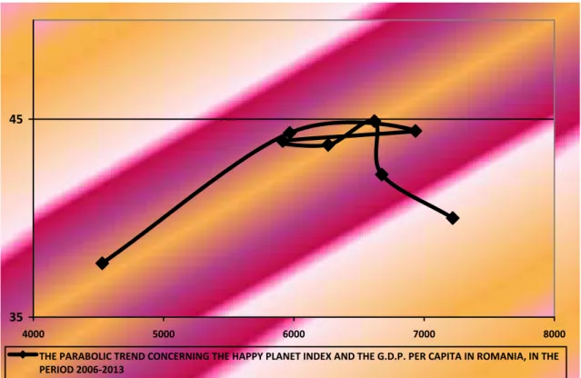
4000 5000 6000 7000 8000

THE PARABOLIC TREND CONCERNING THE HAPPY PLANET INDEX AND THE G.D.P. PER CAPITA IN ROMANIA, IN THE PERIOD 2006-2013

The type no. 2 The trend model of the values for the correlation between the Happy Planet Index and the G.D.P. per capita in Romania, in the period 2006-2013

We observe that, the cloud of points which reflects the values of the (appy Planet )ndex in Romania in function of the G.D.P. per capita in Romania, between - , it carrying around a quadratic trend model, according to the type no. .

4. The intensity of the correlation between the G.D.P. per capita in Romania and the Happy Planet Index in Romania, in the period 2006-2013

For to reflect the intensity of the quadratic correlation between the G.D.P. per capita in Romania and the(appy Planet )ndex in Romania, between - , we use the Correlation Raport noted with

η

[ ]:

Table no. 9 The calculation of the value for the Correlation Raport in the case of the quadratic correlation between the G.D.P. per capita in Romania and the Happy Planet Index

in Romania, between 2006-2013

YEARS THE G.D.P. PER CAPITA

IN ROMANIA

(EURO) (

ξ

i)

THE HAPPY PLANET INDEX

IN ROMANIA

(

ω

i)

i

i

ω

ξ

2

2

i

ω

ξ

i

ω

i

2006 4.530 37,72 . . . , ,

2007 5.969 44,30 . . . . , ,

2008 6.933 44,40 . . . . , ,

2009 5.915 43,90 . . . . , ,

2012 6.675 42,20 . . . . , ,

2013 7.220 40,00 . . . . , ,

TOTAL 50.123 341,12 . . . . , ,

n

n

c

b

a

n

i i n

i i

n

i i

i i n

i i i n

i i

2

1 1

2

2

1 2

1 1

⎟

⎠

⎞

⎜

⎝

⎛

−

⎟

⎠

⎞

⎜

⎝

⎛

−

+

+

=

∑

∑

∑

∑

∑

∑

=

=

=

= =

ω

ω

ω

ω

ξ

ω

ξ

ω

η

(

)

(

)

0,99972

8 12 , 341 3984 , 590 . 14

8 12 , 341 0 1366855266 )

88582 0000026392 ,

0 ( 3 , 2144118 7

0323079270 ,

0 12 , 341 ) 56910975 ,

54 (

2

2

= −

− ⋅

− + ⋅

+ ⋅ −

=

)n conclusion, because the value of the Correlation Raport tends to , there is a very strong intensity of the relationship between the Gross Domestic Product per capita in Romania and the (appy Planet )ndex in

Romania, between - .

5. Conclusions

We can to synthesize that, there is a correlation of parabolical type between the values of the Gross Domestic Product per capita in Romania and the values of the (appy Planet )ndex in Romania, between - . Also, there is a strong intensity of the correlation between the G.D.P. per capita and the (appy Planet )ndex in Romania, in the period - , because the G.D.P. per capita represents a measure of the societal progress and the effects of him development can be observed on values regarding the (appy Planet )ndex.

References

1. Gauss C. F. - „Theoria Combinationis Observationum Erroribus Minimis Obnoxiae”, Apud Henricum Dieterich Publising House, Gottingae, 1823.

2. Kariya T., Kurata H. - „Generalized Least Squares”, John Wiley&Sons Publishing House, Hoboken, 2004.

3. Pearson K. - „On the General Theory of skew correlation and non-linear regression”, Dulau&Co Publishing House, London, 1905. 4. Wolberg J. - „Data Analysis Using the method of Least Squares: Extracting the Most Information from Experiments”, Springer-Verlag