Modern Gravity Models of Internal Migration. The Case of Romania

(1)

Modern Gravity Models of Internal Migration.

The Case of Romania

Daniela BUNEA Bucharest Academy of Economic Studies [email protected]

Abstract. Internal migration, although less investigated than international migration, is a key mechanism for adjustment to regional economic shocks, especially when other tools prove useless. But this process has very complex factors of determination which can be economic, social, demographic, environmental, etc. Based on previous international studies, in the case of Romania the robust variables proved to be the population size, the per capita gross domestic product, the road density, an amenity index and the crime rate from a static perspective, and the previous migration, the population size and the amenity index from a dynamic perspective. The techniques I have employed in making this study are the Least Square Dummy Variables (LSDV, or the fixed effects method) and the Generalized Method of Moments (GMM, or the dynamic method) both applied to panel data.

Keywords: internal migration; gravity model; panel data; fixed effects method; dynamic method.

JEL Codes: J61, R2, C33. REL Codes: 9J, 9G.

(2)

1. Internal migration: approaches, typology, perspectives and theories

Migration is not a random process. It is a rational choice that implies two decisions: to migrate and where to migrate. The first represents the microeconomic approach, while the second refers to the macroeconomic approach. They are both independent and sequential decisions. The purpose of the micro approach is the individual’s behaviour and the factors which influence its migration decision; instead, the macro approach refers more to places rather than people and to aggregate flows of migrants rather than individual ones. Migration comprises three main contexts:

 spatial context distinguishes between internal and international migration;

 modelling context distinguishes between micro and macro approaches;

 context of the purpose distinguishes between identifying the determinants of migration and exploring the consequences of migration (Etzo, 2008, pp. 1-27).

Migration can take two forms: speculative migration and contracted migration. The former consists in searching for a job in another place, while the latter is provoked by already finding a job in another place (Silvers, 1977, pp. 29-40). Molho (1986, pp. 396-419) considers that speculative migration is part of the job-search process whereas contracted migration is the result of this process.

In the literature there are two perspectives on internal migration: the disequilibrium perspective and the equilibrium perspective. The former argues that migration is due to the existence of regional salaries that do not clear (adjust, equilibrate) the market, whereas the latter considers that regional variations do clear the market. Although both views consider spatial variations of utility that underlie migration, they differ in the source and persistence of these variations (Greenwood, 1997, pp. 648-720).

(3)

accommodation costs, etc.) (Borjas, 2008, pp. 321-364). If the neoclassical theory argues that migration takes place before finding a job at destination, the job-search (job-matching) theory argues that migration occurs after having already a job in hand. While job-search theory considers individual decision, job-matching theory considers aggregate decision. The human capital (neoclassical) model cannot explain by itself the migration process because it assumes that information is costless. So, the migration decision should be taken in two stages: first, to migrate or not, taking into account the costs involved; second, to accept or not a certain job (Jackman and Savouri, 1992, pp. 1433-1450). Finally, the Keynesian theory is critical against the neoclassical one due to the different view on money. Therefore, according to the Keynesian economists, labour supply depends not only on real wage (as argued by the neoclassical economists), but also on nominal wage. Thus, migrants are also attracted by high nominal wage regions. Moreover, if in the neoclassical approach migration reduces real wage disparities among regions, in Keynesian approach migration reduces rather unemployment disparities (Jennissen, 2007, pp. 411-436).

Migrants are not randomly sorted out because of differences in migration costs each of them bears and of the shape of income distribution in any two regions (origin and destination). Related to this last fact, the selection of migrants can be of two types:

 Positive selection, when:

- migrants have above-average skills;

- destination offers a higher rate of return to skills than origin;

- migrants are chosen from the upper tail of the skill distribution ladder because origin “taxes” high-skilled workers and “insures” low-skilled workers against poor labour market outcomes.

 Negative selection, when:

- migrants have below-average skills;

- origin offers a higher rate of return to skills than destination;

- migrants are chosen from the bottom tail of the skill distribution ladder because origin “rewards” high-skilled workers and “punishes” less-skilled workers.

(4)

2. Gravity models and possible determinants of internal migration. Literature review

Newton´s law about universal gravitation (1687) states that the attractive force between two bodies is directly related to their size and inversely related to the distance between them. Newton´s law was applied to migration research by Lowry (1966, pp. 1-118) and Lee (1966, pp. 47-57). The basic gravity model can be applied to migration as follows:

 in mathematical form:

D P P g M ij j i ij _  _ 

 , or (1)

 in statistical form (in logs):

            

 log(g) log(Pi) log(P j) log(Dij) ij

Mij ₍₂₎

where Mij is the migration from region “i” to region “j”, Pi and Pj the origin and destination populations, Dij the physical distance between “i” and “j”, α-β-χ elasticities, and g a gravitational constant. Newton considered that α = β = 1 and

χ = 2.

Since Lowry (1966, pp. 1-118), the basic gravity model has been extended to the following form:

, ij ) Dij log( 5 ) X j log( 4 ) Xi log( 3 ) P j log( 2 ) Pi log( 1 ) g log( 0 Mij                      (3)

where Xi is a vector of explanatory variables describing different features of the origin (i.e. push factors) and Xj is a vector of explanatory variables describing features of the destination (i.e. pull factors). Push factors are those characteristics of the origin place that encourage (discourage) out-migration (in-migration), such as low incomes, high unemployment, high prices, in general few opportunities for development. Instead, pull factors are those characteristics of the destination place that encourage (discourage) in-migration (out-migration).

(5)

A very complex classification of internal migration determinants was made by Van der Gaag et al. (2003, pp. 1-141) which make the difference between “those characteristics of individuals or households that are indicative of higher or lower propensities to migrate and those factors that actually determine whether a move takes place and which destination is selected” (p. 12). Therefore, there are both selective influences (demographic factors) and determinants of migration. The demographic factors include mainly age and sex. If age is variable, sex is a constant. Migration tends to be higher for young children, decreases at school-leaving age and rises again at labour force entrance. Many studies insist that migration declines with age except for when older persons need family help or medical aid. Even though sex differences are not as significant as those between ages, the empirical evidence shows that women rates could be higher than men´ after the age of 16, after which could fall below men´ until the retirement age; finally, in older old age, female rates could again exceed those of males (for further details see Van der Gaag et al., 2003, pp. 1-141).

Migration determinants can be classified in: gravity variables, economic variables, labour market variables, real estate variables, environment variables and political variables. Gravity variables are population sizes, with positive influences, and physic distance, with negative influence. Economic variables could be numerous: gross domestic product per capita, newly created businesses, wages, etc. Labour market variables include: levels and/or rates of (un)employment, changes in working conditions, etc. Housing market variables act in the following manner: high prices of houses and low vacancy rates deter migration unless anticipated by potential migrants; size, structure and quality of residential stock affect level and type of migration, and also construction and demolition rates. Environment variables are those that affect quality of life both on short and long term, among these being terrain conditions (abandoned, vacant, greenfield, or brownfield), population density, degree of urbanization, social behaviour of local inhabitants, climatic conditions, leisure and entertainment activities, etc.. Policy variables refer to governmental subsidies, local taxes, defense spending, educational offer, urban area plan, or direct measures such as migration incentives and policies. One should bear in mind that there is no strict delimitation between these variables (Van der Gaag et al., 2003, pp. 1-141).

Instead, Borjas (2000, pp. 1-21), in Economics of migration, considers the following general determinants of internal migration:

(6)

 Education: highly educated people are eager to migrate because they are more efficient in assessing employment opportunities in various labour markets, thus reducing migration costs.

 Distance: the longer the distance the lower the incentive to migrate due to larger migration costs.

 Other factors: unemployment – the unemployed are more likely to migrate; suffers from endogeneity problems; wage differentials – potential positive impact is sensitive to selection bias problems.

In applying the gravity model represented above, almost all studies employed as dependent variable the gross migratory flows from origin “i” to destination “j”.

Anjomani (2002, pp. 239-265) carried out an analysis of US interstate migration and included as regressors the following variables grouped as follows:

 Previous gross migration, as a proxy for social networks or availability of information, it should impact positively; information decreases with increased distance and increases if in the past more people migrated from origin “i” to destination “j”; relatives and friends may facilitate the journey of the recent migrant by providing him initial accommodation and information about job prospects;

 Economic variables: regional income, employment rate, unemployment rate, local income tax;

 Amenity variables: population density, mean temperature, welfare benefits, criminality rate;

 Demographic variables: population size or growth, mean educational level, median population age.

As technique of estimation he used Two Stage Least Square (2SLS). Ivan Etzo (2008, pp 1-29) investigated the determinants of interregional migration in Italy by using population size, distance between main cities, GDP per capita, unemployment rate, infrastructure index and crime rate in both origin and destination regions. The techniques employed were the Fixed Effects Vector Decomposition Estimator (FEVD) and the Generalised Method of Moments (GMM).

(7)

Parikh and Van Leuvensteijn (2002, pp. 1-22) carried out a panel data analysis for the regions of Germany and employed variables like unemployment rate differential, unemployment rate, wage differential for blue-collar workers and wage differential for white-collar workers (in logs), differential in hospital and hotel beds per inhabitant, differential in per capita rented or owned housing, differential in rental price per km2, distance between the main cities and differential in cost of living index. The econometric methods used were Least Square Dummy Variables (LSDV) and GMM.

3. Internal migration in Romania. Statistical and econometric analyses

All data used in this empirical research are at NUTS 3 level, i.e. county level, because a regional analysis (NUTS 2) would involve serious problems of aggregation due to the different sizes and number of counties each region of Romania comprises. Hence, using NUTS 3 level one can assess movements across counties that would have been impossible to do using NUTS 2 level (Ailenei, Bunea, 2010, pp. 159-164). Therefore, the county analysis will be more relevant and precise.

The period under analysis is 2004-2008.

A. Statistical analysis

(8)

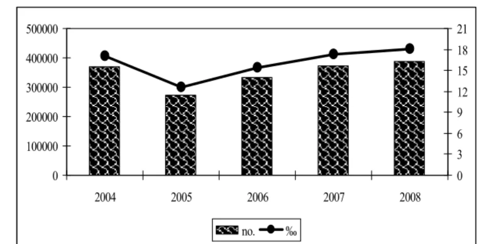
0 100000 200000 300000 400000 500000

2004 2005 2006 2007 2008

0 3 6 9 12 15 18 21

no. ‰

Source: Personal elaboration based on Romanian Statistical Yearbooks 2005-2010.

Figure 1. Gross migration (no. of migrants and rates)

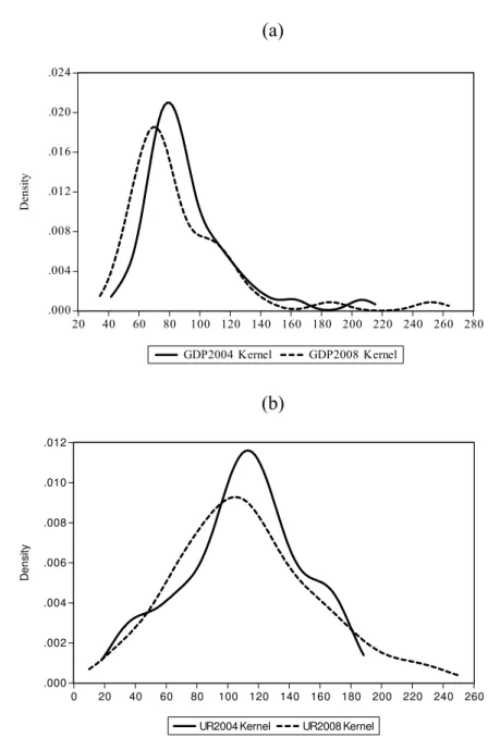
Can this upward trend be explained by increasing differentials in county GDP per capita and/or county unemployment rate? Both GDP per capita and unemployment rate at county level experienced a divergence process (i.e. σ-convergence), as can be seen from the ascending evolution of their coefficients of variation (Figure 2). The kernel density distributions confirm the aforementioned trends (Figures 3(a) and 3(b)). These distributions are computed following the rule of Silverman (1986, pp. 1-22). First, I have transformed the values of GDP in relative terms, with national mean = 100, in order to facilitate comparisons and eliminate the impact of absolute changes over time (Ezcurra, Pascual, 2006, pp. 1-6). Hence, it seems that increasing migration may have its roots in increasing differentials among counties.

0.32

0.382 0.399 0.403

0.433

0.391 0.405 0.404

0.457 0.47

0 0.1 0.2 0.3 0.4 0.5

2004 2005 2006 2007 2008

GDP/capita Unemployment

(9)

(a)

.000 .004 .008 .012 .016 .020 .024

20 40 60 80 100 120 140 160 180 200 220 240 260 280

GDP2004 Kernel GDP2008 Kernel

De

n

si

ty

(b)

.000 .002 .004 .006 .008 .010 .012

0 20 40 60 80 100 120 140 160 180 200 220 240 260

UR2004 Kernel UR2008 Kernel

De

n

s

it

y

Source: Personal elaboration based on Romanian Statistical Yearbooks 2005-2010 and

using EVIEWS 7.

(10)

Counties with the lowest real GDP per capita (2004 prices): Vaslui, Botoşani, Giurgiu, Călăraşi, and Teleorman with a total average of about 38,700 lei per inhabitant. Counties with the highest real GDP per capita: Bucharest, Ilfov, Timiş, Cluj, and Constanţa with a total average of about 114,800 lei per inhabitant. Counties with the highest unemployment rates: Vaslui, Mehedinţi, Ialomiţa, Teleorman, and Gorj with an average of 8.9%. Counties with the lowest unemployment rates: Timiş, Bucharest, Ilfov, Bihor, and Satu-Mare with an average of 2.3%.

Making a simple aggregation, on average, 10 counties with GDP per capita above national average (from a total of 11) had positive balances, whereas 27 counties with GDP below average (from a total of 31) had negative balances. As for unemployment, 10 counties with rates below national average (from a total of 16) had net inflows, whilst 22 counties with rates above average (from a total of 26) recorded net outflows. So, it seems that both high GDP per capita counties and low unemployment counties record net inflows while both low GDP per capita counties and high unemployment counties record net outflows.

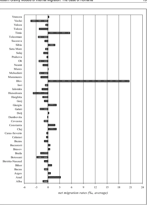
On average, Ilfov, Timiş and Arad were the counties that registered the highest positive rates: 20.6, 5.5 and, respectively, 3.2‰; while Vaslui, Hunedoara and Botoşani recorded the highest negative rates: -4.3, -3.7 and, respectively, -2.7‰ (Figure 4). As for the gross flows, Table 1 presents the counties with the highest and lowest rates.

Table 1

Extreme out and in-migration rates by county

- average 2004-2008 –

Out-migration (‰) In-migration (‰)

minimum Harghita 11.8 Harghita 10.4

Covasna 12.2 Maramureş 10.7

Maramureş 12.5 Brăila 10.9

maximum Bucharest 22.2 Ilfov 34.4

Gorj 20.0 Bucharest 22.8

Vâlcea 18.8 Timiş 21.2

(11)

-6 -3 0 3 6 9 12 15 18 21 24 Alba

Arad Arges Bacau Bihor Bistrita-Nasaud Botosani Braila Brasov Bucuresti Buzau Calarasi Caras-Severin Cluj Constanta Covasna Dambovita Dolj Galati Giurgiu Gorj Harghita Hunedoara Ialomita Iasi Ilfov Maramures Mehedinti Mures Neamt Olt Prahova Salaj Satu Mare Sibiu Suceava Teleorman Timis Tulcea Valcea Vaslui Vrancea

net migration rates (‰, average)

(12)

Next map counts 28 counties with negative balances and 14 with positive balances.

Figure 5. County map of migratory balances

B. Econometric analysis

This section employs a panel data technique whose main feature is that each observation varies both across time and across entities (i.e. counties) and it can take better advantage for omitted variables and individual heterogeneity (Baltagi, 2005, pp. 1-302, Wooldridge, 2002, pp. 1-735).

(13)

The next variables were included and tested in model (4) (all in logs and interpreted as elasticities to migration):

 dependent variable (MR): ratio in-migrants / out-migrants;

 independent variables:

- POP: inhabitants of each county;

- GDP: real GDP per capita (in 2004 prices) – proxy for wages; - UR: unemployment rate (number of registered unemployed divided

by each county’s active population) – proxy1 for the probability of finding a job;

- ER: employment rate (number of civil employees divided by each county’s total population) – proxy2 for the probability of finding a job; - HOUSE: private dwelling rate (number of private dwellings per

1,000 inhabitants);

- EDU: university graduates per 1,000 inhabitants – proxy for competition;

- URB: degree of urbanization (urban population divided by rural population);

- AMN: amenities index (length of public sewerage pipes – km2 + length of distribution pipes of natural gas – km2 + length of drinking water supply network – km2 + urban green spaces area – ha per 1,000 inhabitants) – proxy1 for infrastructure;

- ROAD: density of public roads per 100 km2 – proxy2 for infrastructure;

- DEATH: infant deaths per 1,000 live-births – proxy for health care; - DENS: population density (number of inhabitants per km2) – proxy

for crowding and congestion;

- CRIM: criminality rate (number of persons definitively convicted per 100,000 inhabitants) – proxy for social behaviour.

All independent variables are lagged one period in order to avoid endogeneity problems or simultaneity bias. Greenwood (1985, p. 535): “Migration is likely to respond with a lag to changed circumstances”, because it takes time to acquire the necessary information.

This paper uses the following model:

 

 _ci x_Xit _it

MR it    , (4)

where ci is the unobserved effect, i.e. characteristics that vary between counties but are constant over time, and Xit is the vector of all regressors (covariates) mentioned above.

(14)

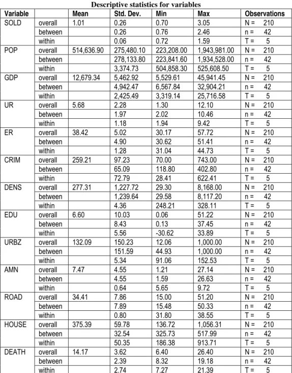
Table 2

Descriptive statistics for variables

Variable Mean Std. Dev. Min Max Observations

SOLD overall 1.01 0.26 0.70 3.05 N = 210

between 0.26 0.76 2.46 n = 42

within 0.06 0.72 1.59 T = 5

POP overall 514,636.90 275,480.10 223,208.00 1,943,981.00 N = 210 between 278,133.80 223,841.60 1,934,528.00 n = 42 within 3,374.73 504,858.30 525,608.50 T = 5 GDP overall 12,679.34 5,462.92 5,529.61 45,941.45 N = 210

between 4,942.47 6,567.84 32,904.21 n = 42 within 2,425.49 3,319.14 25,716.58 T = 5

UR overall 5.68 2.28 1.30 12.10 N = 210

between 1.97 2.02 10.46 n = 42

within 1.18 1.94 9.42 T = 5

ER overall 38.42 5.02 30.17 57.72 N = 210 between 4.90 30.62 51.41 n = 42

within 1.28 31.04 44.73 T = 5

CRIM overall 259.21 97.23 70.00 743.00 N = 210 between 65.09 118.80 402.80 n = 42 within 72.79 28.41 622.41 T = 5 DENS overall 277.31 1,227.72 29.30 8,168.00 N = 210

between 1,239.64 29.58 8,117.20 n = 42 within 4.36 248.21 328.11 T = 5 EDU overall 6.60 10.03 0.06 51.22 N = 210

between 8.43 0.13 37.45 n = 42

within 5.56 -30.62 33.89 T = 5 URBZ overall 132.09 150.23 12.06 1,000.00 N = 210

between 151.59 44.93 1,000.00 n = 42 within 5.34 91.06 152.53 T = 5 AMN overall 7.47 4.55 1.21 27.14 N = 210

between 4.55 1.59 26.63 n = 42

within 0.64 5.65 9.72 T = 5

ROAD overall 34.41 7.86 15.00 51.20 N = 210 between 7.89 15.48 50.33 n = 42

within 0.80 31.80 38.55 T = 5

HOUSE overall 375.39 59.78 136.72 1,056.31 N = 210 between 32.54 325.73 517.99 n = 42 within 50.35 186.38 913.71 T = 5 DEATH overall 14.17 3.62 6.40 26.40 N = 210

between 2.39 8.32 19.18 n = 42

within 2.74 7.27 21.39 T = 5

Source: Personal elaboration based on Romanian Statistical Yearbooks 2005-2010 and

(15)

i. Static approach: Fixed effects regressions

First, let´s introduce some information about Least Square Dummy Variables (LSDV) or Fixed Effects method. FEM assumes ci to be

deterministic, thus correlated with the covariates, and is based on the within estimation, i.e. each observation is within the county ´i´ throughout the period. Instead, the random effects model (REM) assumes ci to be stochastic (random),

thus not correlated with the covariates and included in the error term. Another way put, the REM estimates are consistent only if ci are independent or

uncorrelated with the regressors or with the error term (Wooldridge, 2002, pp. 1-735). Applying Hausman test (1978) in order to establish the consistency of REM estimates, under the null hypothesis that cov(X_it,c_i) =0, the output invalidated the consistency of REM.

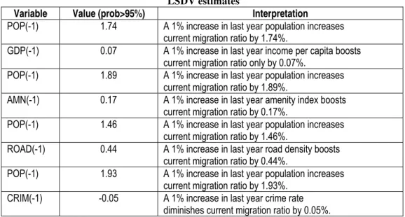
I have employed STATA 9 and EVIEWS 7 to perform FEM regressions. After controlling for the population effect (significant), the significant variables turned out to be: real GDP per capita, amenity index, road density and crime rate (Table 3).

Table 3

LSDV estimates

Variable Value (prob>95%) Interpretation POP(-1) 1.74 A 1% increase in last year population increases

current migration ratio by 1.74%.

GDP(-1) 0.07 A 1% increase in last year income per capita boosts current migration ratio only by 0.07%.

POP(-1) 1.89 A 1% increase in last year population increases current migration ratio by 1.89%.

AMN(-1) 0.17 A 1% increase in last year amenity index boosts current migration ratio by 0.17%.

ROAD(-1) 0.44 A 1% increase in last year road density boosts current migration ratio by 0.44%.

CRIM(-1) -0.05 A 1% increase in last year crime rate diminishes current migration ratio by 0.05%.

ii. Dynamic approach: two-step GMM regressions

(16)

regressions with different lags. The strictly exogenous variables are those unaffected by past, current and future shocks/errors and all will be instrumented. The predetermined variables are those independent of current disturbances but possibly affected by past ones and will be instrumented with lag 1 and earlier; this is the case of all our covariates. Finally, the endogenous variables are those correlated with the current errors; these will be instrumented from lag 2 onward. GMM estimators are corrected for heteroskedasticity bias and endogeneity between variables (Roodman, 2006, pp. 1-51).

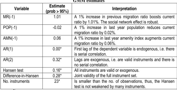
The following results were obtained using STATA 9. After controlling for the population effect (significant), the only significant variable turned out to be the amenity index. The valid instruments are the migration ratio from lag 2 onward, the population size and the amenity index both from lag 1 onwards. The robustness of the amenity index resides in the tiebout hypothesis: people “vote with their feet” in search of better provision of local public goods (Andrienko, Guriev, 2003, pp. 1-31).

Apart from the amenity index significance, results reported in Table 4 also reveal the importance of the social network theory, i.e. interpersonal relations due to friendship, kinship, or a shared community of origin which may help increasing migration due to the reduction in information asymmetry or in costs and risks (a shelter, food, available jobs, etc.) (Anjomani, 2002, pp. 239-265).

Table 4

GMM estimates

Variable Estimate

(prob > 95%) Interpretation

MR(-1) 1.01 A 1% increase in previous migration ratio boosts current ratio by 1.01%. The social network effect is robust.

POP(-1) -0.02 A 1% increase in last year population reduces current migration ratio by 0.02%.

AMN(-1) 0.06 A 1% increase in last year amenity index augments current migration ratio by 0.06%.

AR(1) 0.00* First lag of the dependent variable is endogenous, i.e. there is serial correlation.

AR(2) 0.32* Lags are exogenous, i.e. are valid instruments and there is no serial correlation.

Hansen test 0.16* All instruments are valid or exogenous. Joint validity of the full instrument set. Difference-in-Hansen 0.28*

No. instruments 23* Is smaller than the no. of observations, thus, the Hansen test is not weakened by many instruments.

*)

(17)

4. Final remarks

In this paperwork I have tried to investigate on the potential determinants of internal migration in Romania using county data for the period 2004-2008. The main results pointed out significant impacts of population size, real gross product per capita, amenity index, road density and crime rate from a static point of view, and significant effects of previous migration ratio, population size and amenity index from a dynamic point of view. All variables returned the correct signs.

Following this study, I plan to search for other possible determinants and to apply additional techniques of estimation in order to compare different outcomes and obtain an accurate assessment as possible of our domestic migration.

Acknowledgements

This article is carried out under the project “PhD in Economics at Standards of the Europe of Knowledge” (DoEsEC), POSDRU/88/1.5/S/55287, co-financed by the European Social Fund and implemented by Bucharest Academy of Economic Studies in partnership with West University of Timişoara.

References

Ailenei, D., Bunea, D., “Labour market flexibility in terms of internal migration”, Annals of University of Oradea, Economic Science, TOM XIX, no. 1, 2010

Andrienko, Y., Guriev, S., “Determinants of interregional mobility in Russia: Evidence from panel data”, Working Paper, No. 551, 2003, The William Davidson Institute

Anjomani, A., “Regional growth and interstate migration”, Socio-Economic Planning Science, vol. 36, 2002

Baltagi, B.H. (2005). Econometrics analysis of panel data, ed. 3, John Wiley & Sons Ltd, Chichester Borjas, G.J., “Economics of migration”, International Encyclopedia of the Social & Behavioral

Sciences, 2000

Borjas, G.J. (2008). Labor economics, Ed. 4, McGraw-Hill/Irwin, New York

Decressin, J.W., “Internal migration in West Germany and implications for east-west salary convergence”, Weltwirtschaftliches Archiv, vol. 130, 1994

Etzo, I., “Determinants of interregional migration in Italy: A panel data analysis”, MPRA Paper, No. 8637, 2008, pp. 1-29, University Library of Munich, Germany

Etzo, I., “Internal migration: a review of the literature”, MPRA Paper No. 8783, 2008, pp. 1-27,

University Library of Munich, Germany

(18)

Ghatak et al., “Inter-regional migration in transition economies: The case of Poland”, Discussion Paper, No. 7, 2007, pp. 1-29, School of Economics, Kinston University, London,

Greenwood M.J., 1985. “Human migration: Theory, models and empirical studies”, Journal of Regional Science, vol. 25, pp. 521-544

Greenwood, M.J., 1997 – Ch. 12. “Internal migration in developed countries”, in Rosenzweig, M. R. and Stark, O. (eds.), 1997, Handbook of Population and Family Economics, vol. 1B, pp. 648-720, Amsterdam, Elsevier

Hicks, J.R. (1932). The theory of wages,Macmillan, London

Jackman, R., Savouri, S., “Regional migration in Britain: An analysis of gross flows using NHS central register data”, Economic Journal, vol. 102, 1992

Jennissen, R., “Causality chains in the international migration systems approach”, Population Research and Policy Review, vol. 26, 2007

Lee, E.S., “A theory of migration”, Demography, vol. 3, 1966

Lowry, I. (1966). Migration and metropolitan growth: two analytical models, Chandler Publishing Company, San Francisco

Molho, I., “Theories of migration: a review”, Scottish Journal of Political Economy, vol. 33, 1986 Parikh, A., Van Leuvensteijn, M., “Internal migration in regions of Germany: A panel data analysis”,

Working Paper, No. 12,2002, European Network of Economic Policy Research Institutes Roodman, “How to Do xtabond2: An introduction to Difference and System GMM in Stata”,

WorkingPaper, No. 103, 2006, Center for Gobal Development

Silverman, B.W. (1986). Density estimation for statistics and data analysis, pp. 1-22, Chapman and Hall, London

Silvers, A., “Probabilistic income maximizing behaviour in regional migration”, International Regional Science Review, vol. 2, 1977

Van der Gaag, N. et al., “Study of past and future interregional migration trends and patterns within European Union countries in search of a generally applicable explanatory model”, Report on behalf of Eurostat, 2003

Wooldridge, J.M. (2002). Econometric Analysis of Cross-Section and Panel Data, MIT Press, Massachusetts