The Case of Hungary (1981–2006)
Aleksandar VasilevAmerican University in Bulgaria avasilev@aubg.edu
This paper investigates for the presence of a New Keynesian Phillips (nkpc) curve in Hungary in the period 1981:3–2006:2. The empirical model we test features forward-looking firms who pre-set prices for a cou-ple of periods ahead, using Calvo (1983) pricing rule. We also estimate a hy-brid version of nkpc, where some of the firms are backward looking, and others are forward-looking in their price-setting behaviour. Real marginal costs and forward-looking behaviour are statistically significant and quan-titatively important in the nkpc. However, there are some econometric is-sues to be considered, such as the weak identification of the parameters of the structural nkpc as well as those of the hybrid nkpc.
Key Words:New Keynesian Phillips curve, Hungary, instrumental non-linear gmm Estimation, weak identification
jel Classification:c22, c2, e24
Introduction
This paper investigates for the presence of a New Keynesian Phillips (nkpc) curve in Hungary in the period 1981:3–2006:2. Hungary is a unique case among the transition economies as a country that traded freely with Western European countries even before the fall of the social-ist regime, and thus is an interesting case of study. Under that regime, export firms had to use market prices in order to be competitive and gain market share in Western Europe. In that sense, we can regard the behaviour of exporting firms as closely resembling the behaviour of a profit-maximizing Western firm operating in a competitive environment. Therefore, we will adopt models developed for the us to study the dy-namics of inflation in this transition country.
tested features forward-looking firms who pre-set prices for a couple of periods ahead, using Calvo (1983) pricing rule. In addition, measures of real marginal cost are used instead of the old-fashioned output gap. The reason is that marginal costs are a better proxy for the impact of the pro-ductivity gains on inflation, which the ad hoc measure output gap misses. A hybrid version of nkpc, where some of the firms are backward look-ing, and others are forward-looking in their price-setting behaviour, is also estimated.
Despite the presence of a substantive literature on the subject of nkpc in Hungary (Menyhert 2008; Vasicek 2011; Franta, Saxa, and Smidkova 2010), earlier studies either take a much shorter time span (Menyhert 2008; Vasicek 2011), or focus on inflation persistence (Franta, Saxa, and Smidkova 2010). In this paper the emphasis is on the transition expe-rience of Hungarian economy (hence the time period that is chosen), and not on inflation forecasting. In addition, the paper touches upon the problem of weak identification, which previous studies do not discuss. Therefore, given the different focus of the paper, the results from earlier studies are not directly comparable.
The paper is organized as follows: the second section describes Gali and Gertler’s (1999) approach and, thus provides a brief review of the theory that gave rise to the new Phillips curve, and discusses some ex-isting empirical results. The third Section contains the estimates of the new Phillips curve. In the fourth section, the model is extended to al-low for backward-looking firms and results of a so-called ‘hybrid Phillips curve’ are presented. The fifth section concludes.
The New Phillips Curve: Background Theory and Evidence The setup of the model features monopolistically competitive firms who face some constraints on price adjustments. The price adjustment rule is time-dependent – every period a fraction 1/Xof firms set their prices for Xperiods ahead in the spirit of Taylor (1980). In order to keep track of the histories of all firms we use Calvo pricing (1983) rule, which simplifies the aggregation problem: in any given period, each firm has a fixed probabil-ity 1−θthat it may adjust its price during that period. Therefore, the aver-age time over which a price is fixed is given by (1−θ)∞k=0kθk−1=1/(1−θ). Another common assumption is that the monopolistically competitive firm faces a constant price elasticity of demand curve. Then, Gali and Gertler (1999) show that the aggregate price levelptevolves as a convex
(the price selected by firms that are able to change the price at periodt). Therefore, the pricing rule takes the following form:
pt =θpt−1+(1−θ)pt*. (1)
Letmcnt be the firm’s marginal costs (as a percentage deviation from the steady state) andβdenotes the discount factor. Each firm chooses a price attto maximize expected discounted profits subject to the Calvo pricing rule, so the optimal reset price is:
pt*=(1−βθ)
∞
k=0
(βθ)kEt{mcnt+k}. (2)
Now letπt = ptpt−1 denote the inflation rate. Combining (1) and (2),
Gali and Gertler (1999) obtain the following equation for the inflation dynamics, or the ‘traditional forward-looking New Keynesian Phillips curve.’
πt=λmct+βEt{πt+1}, (3)
whereλ=(1−θ)(1−βθ)/θdepends on the frequency of priceθadjustment and the discount factorβ. Iterating forward for inflation they obtain
πt=λ ∞
k=0
βkEt{mcnt+k}<∞. (4)
Therefore, the theory says inflation is a discounted stream of expected future marginal costs. Note that the sum above is finite due to the dis-counting effect and the assumption that marginal costs are bounded in each time period.
Traditional Phillips curve emphasizes the use of a proxy for real activ-ity, namely the ‘output gap,’ or the observed gdp series less of a trend. In other words, this is a measure, which shows how current gdp differs from the potential one. It is obtained by taking logs from the series, sea-sonally adjusting the quarterly series, differencing to eliminate the unit root and applying the Hodrick-Prescott filter so that we express it as a percentage change from the steady state. Thus,mct =kxt, wherekis the
elasticity of the marginal cost. Plugging the expression above into the in-flation equation, we obtain
Substituting forward, the resulting expression becomes
πt=λk ∞
k=0
βkEt{mcnt+k}. (6)
It is widely known fact that conventional measures of the output gap contain a substantial amount of measurement errors. That is primarily because the theoretical measure of ‘natural level’ of output is not an ob-servable. The gap is estimated by fitting a smooth deterministic trend and subtracting it from the series. This trend fitting itself involves mea-surement error. Depending on whether supply or demand shocks are predominant in the economy, estimation could lead to counter-intuitive signs of the coefficients.
Gali and Gertler (1999) concentrate on obtaining a measure for real marginal costs, estimated in a way that it is consistent with theory. Their theory is used as a guide for the estimation in this paper: Output is as-sumed to be produced by A Cobb-Douglas production function,Yt = AtKtαkN
αn
t , where At denotes total factor productivity, Kt capital, and
Nt labour. Real marginal cost (mc) is the ratio of the real wage to the
marginal product of labour (mpl). Thus, mct = (Wt/Pt)(∂Yt/∂Nt) = St/αn, whereSt = (WtNt/PtYtis the labour income share. Using
lower-case letters to denote percent deviation from the steady state, the formula becomesmct = st. That measure is obtained by first taking natural logs
from the series and then applying the Hodrick-Prescott filter to it. This series, as well as the series for inflation, is stationary: Dickey-Fuller test rejects the presence of a unit root at 1 level of significance.
After plugging the expression for real mc into the inflation equation, we obtain
πt=λst+βEt{πt+1}. (7)
Since this is a rational expectations (re) model, the forecast ofπt+1is uncorrelated with any of the variables in the information set, i.e. variables in timetor earlier. This leads to the following moment condition
Et{(πt−λst−βπt+1)zt}=0, (8)
whereztis a vector composed of the variables taken from the information
table 1 Reduced-Form Estimates
Proxy for real mc β λ J-statistic p-value
ln_ulc_hp . –. . .
(.) (.)
ln_shlabor_hp . . . .
(.) (.)
dlgdp_sa_hp . –. . .
(.) (.)
notes N=100,df =7.
An important reason why gmm estimation is used is that non-linear least squares (nlls) will give biased and inconsistent estimates since corr(πt,πt+1)0, and thuscorr(εt,πt+1), which violates one of the
under-lying assumptions for using nlls. Note that using nlls-iv estimation with homoscedasticity assumption and no autocorrelation yields exactly the gmm orthogonality condition.
The data used is quarterly for Hungary over the period 1981:3–2006:2. Estimation results are presented in the next section. Forst, natural
loga-rithm of the labour income share is used. Inflation is measured as a per-centage change in the Consumer Price Index (cpi), seasonally adjusted and differenced in order to eliminate the unit root in the series. The in-strument set includes four lags of inflation, the labour income share, the output gap, the long-short interest rate spread, wage inflation and the growth in money supply (m1 aggregate).
The New Phillips Curve: Estimation
We first estimate the reduced from equation, which involves onlyλand β, but not the structural parameterθ, which was the measure of price rigidity. In addition, Appendix 1 checks the identification of the model parameters. Three cases are considered, with log of cyclical component of unit labour costs (ln_ulc_hp), log of cyclical component of the labour share (ln_shlabor_hp), and the differenced log of seasonally adjusted output gap (dlgdp_sa_hp), respectively, as a proxy for real marginal costs. Results are provided in table 1, where the Newey-West estimate of the covariance matrix was used to provide robust standard errors.
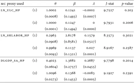
table 2 Estimates of the New Keynesian Phillips Curve
mc proxy used θ β λ J-stat p-value
ln_ulc_hp () . . –. . .
(.) (.) (.)
() . . . .
(.) (.) (.)
ln_shlabor_hp () . . . . .
(.) (.) (.)
() . . . . .
(.) (.) (.)
dlgdp_sa_hp () . . . . .
(.) (.) (.)
() . . –. . .
(.) (.) (.)
notes (1) Case 1. (2) Case 2.N=100,df =7.
should not generate a nkpc when quarterly data was used. In order to recover the structural estimate ofθ non-linear instrumental gmm was also estimated. Fuhrer and Moore (1995) show that in small samples gmm is sensitive to the nature of normalization of the orthogonality conditions. In this paper the ones used by Gali and Gertler (1999) are used:
Et{(θπt−(1−θ)(1−βθ)st−θβπt+1)zt} (9)
and
Et{(πt−θ−1(1−θ)(1−βθ)st−βπt+1)zt} (10)
Their claim is that (9) minimizes non-linearities, while in (10) the co-efficient of inflation in the current period is restricted to be one. We do each specification for (log) labour share, (log) unit labour costs and out-put gap.
The results are reported in table 2, where cases [1] and [2] denote spec-ifications (9) and (10), respectively. The first two columns give the esti-mates of the structural parametersθandβ, and the third provides the es-timate forλ. Standard errors forλwere obtained using the delta method. J-statistic for over-identifying restrictions is also provided. At 5 level of significance, the model is always correctly specified.
esti-mate ofθis unity (all the firms adjust), 0.3 in the case of log-labour income share, and 0.4 in the regression with the output gap. The estimates forλ andβare in the majority of the cases not statistically different from zero. Generally, estimates are very sensitive to the g mm normalization pro-cedure, and sometimes to the initial values chosen. The problem was that the program gives highly negative and statistically significantβ, which is in conflict with the economic logic. The reason is that the reduced form model is identified, while the structural one is not. The latter has multi-ple solutions, and that is formally shown in the appendix. Therefore doing Continuous Updating (cu) will not solve the problem. Using Maximum Likelihood Estimation (mle) is also of no help since the identification issue is not solved. Mavroeidis (2007) points out that Wald and lr test are not robust to failure of the identification assumption. That is a seri-ous issue to be considered for all Neo-Keynesian economists who have nkpc equation in their models. In a very recent working paper, Boug, Cappelen, and Swensen (2007) show that the estimate surface is flat; this finding is a sign of a weak identification. Hendry (2004) also advises that nkpc specification be used with caution.
In the other camp, Martins and Gabriel (2005) try to save the model by using Generalized Empirical likelihood. Stock and Wright (2000) de-velop confidence set estimation to fix weak identification. They admit, however, encountering problems with fixing Wald statistics. It is worth noting that Gali and Gertler (1999) do not discuss this econometric prob-lem. They only mention several other reasons that may cause the estimate ofθ, to have an upward bias. The first one is statistical: our measures of the real marginal cost are just proxies, and thus contain measurement error. Thus, the parameterλis biased towards zero, and appears insignificant, while in reality mc is an important factor for determining inflation. The second reason lies in the theory, which serves as a basis for the model. It assumes a constant mark-up of prices over mc. If mark-up is allowed to vary over the business cycle, however, then price setting becomes less sensitive to mc, and this explains whyλis not statistically significant as well. In a recent paper, Gali, Gertler, and Lopez-Salido (2005) still claim their results are robust, again failing to mention the identification issue.
Hybrid Phillips Curve
Inflation in data features a significant amount of inertia. Thus, in this section we extend the basic Calvo model, and allow for inertia in inflation. Now the environment includes two groups of firms – not only forward-looking, but also backward-looking ones. The latter use a rule of thumb (behave in an adaptive way) when setting prices. In this case, we can see what share of firms is not optimizing, and therefore not acting rationally. We the share of the backward-looking firms is denoted byω. The ag-gregate price level now evolves according to the following formula
pt=θpt−1+(1−θ)pt*, (11)
wherept* is an index of the prices that were reset in periodt. Letpft de-note the price set by a forward-looking firm attandpt
t the price set by
a backward-looking firm. Then the index of the newly set prices may be expressed as
pt*=(1−ω)pft+ωpbt. (12)
Accordingly,pft may be expressed as
pft =(1−βθ) ∞
k=0
(βθ)kEt{mcnt+k}. (13)
Gali and Gerler derive a rule based on the recent pricing behaviour of the competitors as
pbt =pt−1*+πt−1. (14)
Then they obtain the hybrid Phillips curve by combining (13) and (14),
πt=λmct+γfEt{πt+1}+γbπt−1, (15)
whereλ = (1−ω)(1−θ)(1−βθ)φ−1,γf = βθφ−1,γb = ωφ−1, andφ =
θ+ω[1−θ(1−β)].
Note that when ω = 0, this means that all the firms are forward-looking, and we are back to the nkpc. While the reduced form in this case is identified, the hybrid nkpc is adds another dimension of non-linearity and makes the identification problem even more severe.
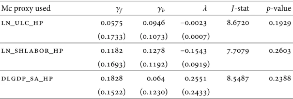
table 3 Hybrid nkpc Reduced-Form Estimates
Mc proxy used γf γb λ J-stat p-value
ln_ulc_hp . . –. . .
(.) (.) (.)
ln_shlabor_hp . . –. . .
(.) (.) (.)
dlgdp_sa_hp . . . . .
(.) (.) (.)
notes N=100,df =6.
costs and output gap as well. Appendix 2 checks the identification of the model parameters. In this case, the model takes the following form
πt=λst+γfEt{πt+1}+γbπt−1+εt. (16)
As seen from table 3, the gamma coefficients are not significant, while lambda estimates are. However, their sign is negative, which makes no economic sense. Still, theJ-test does no reject the null of correct specifi-cation.
The paper then proceeds with the structural estimation procedure us-ing again non-linear instrumental gmm estimator. As in the previous sections, two alternatives are presented, where the first specification min-imizes non-linearities, while the second restricts the coefficient of infla-tion in the current period to one.
Et{(φπt−(1−ω)(1−θ)(1−βθ)st−θβπt+1)zt}=0. (17)
Et{(πt−(1−ω)(1−θ)(1−βθ)φ−1st−θβφ−1πt+1)zt}=0. (18)
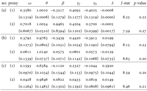
Results are provided in table 4, where [1] and [2] denote specifications (17) and (18), respectively. The automatic choice of the Newey-West co-variance matrix provided robust standard errors.
The estimate ofθis almost everywhere 1, except for the case where the output gap is used, where it is 0.64. All other coefficients are not signif-icant, with the exception for the regression with unit labour cost. That equation, however, gives puzzling results because the share of forward-looking firms is negative, which makes no economic sense. Still, theJ-test confirms that the model is correctly specified.
signif-table 4 Estimates of the New Hybrid Phillips Curve
mc proxy ω θ β γf γb λ J-stat p-value
(a) () . . –. . –. –.
(.) (.) (.) (.) (.) (.) . .
() . . . . . –.
(.) (.) (.) (.) (.) (.) . .
(b) () . . –. . –. .
(.) (.) (.) (.) (.) (.) . .
() . . . . . –.
(.) (.) (.) (.) (.) (.) . .
(c) () . . –. . –. .
(.) (.) (.) (.) (.) (.) . .
() . . . . . .
(.) (.) (.) (.) (.) (.) . .
notes (a) ln_ulc_hp. (b) ln_shlabor_hp. (c) dlgdp_sa_hp. (1) Case 1. (2) Case 2.N=100,df =6.
icant effect of the output gap in a model with many restrictions. One ex-planation, aside from the identification issue, is that compared to the us, Hungary is a small open economy, so firms take international prices as given. In a regime of free trade, those firms have to adjust quickly and act in a very competitive environment, as compared to the us firms, which may be acting indeed as monopolistically competitive producers and can afford to run a band of inaction. Indeed, the degree of backwardness is not statistically different from 0, and mark-up is seriously squeezed (theoret-ically equals the transportation costs of the foreign import companies).
Conclusion
A hybrid version of nkpc, where some of the firms are backward look-ing, and others are forward-looking in their price-setting behaviour, was also estimated. However, there are some econometric issues to be consid-ered, such as the weak identification of the parameters of the structural nkpc as well as those of the hybrid nkpc.
References
Boug, P., A. Cappelen, and A. Swensen 2007. ‘The New Keynesian Phillips Curve Revisited.’ Discussion Paper 500, Statistics Norway, Research Department, Kongsvinger.
Calvo, G. A. 1983. ‘Staggered Prices in a Utility Maximizing Framework.’ Journal of Monetary Economics12 (3): 383–98.
Franta, M., B. Saxa, and K. Smidkova 2010. ‘The Role of Inflation Persis-tence in the Inflation Process in the New eu Member States.’Czech Journal of Economics and Finance60 (6): 480–500.
Fuhrer, J. C. 1997. ‘The (Un)Importance of Forward-Looking Behavior in Price Specifications.’Journal of Money, Credit and Banking29 (3): 338– 50.
Fuhrer, J. C., and G. Moore. 1995. ‘Inflation Persistence.’Quarterly Journal of Economics440:127–59.
Gali, J., and M. Gertler. 1999. ‘Inflation Dynamics: A Structural Estimation Analysis.’Journal of Monetary Economics44 (2): 195–222.
Gali, J., M. Gertler, and D. Lopez-Salido. 2005. ‘Robustness of the Estimates of the Hybrid New Keynesian Phillips Curve.’Journal of Monetary Eco-nomics52 (6): 1107–1118.
Hendry, D. F. 2004. ‘Unpredictability and the Foundations of Economic Forecasting.’ Economics Papers 2004-w15, Economics Group, Nuffield College, University of Oxford, Oxford.
Martins, L. F., and V. Gabriel 2006. ‘Robust Estimates of the New Keynesian Phillips Curve.’ Discussion Papers in Economics 02/06, University of Surrey, Guildford.
Mavroeidis, S. 2007. ‘Testing the New Phillips Curve Without Assuming Identification.’ Working paper, Brown University, Providence, ri. Menyhert, B. 2008. ‘Estimating the Hungarian New Keynesian Phillips
Curve.’Acta Oeconomica58 (3): 295–318.
Roberts, J. M. 1997. ‘Is Inflation Sticky?’Journal of Monetary Economics39 (2): 173–96.
———. 1998. ‘Inflation Expectations and the Transmission of Monetary Policy.’ Mimeo, Federal Reserve Board, Washington, dc.
Taylor, J. B. 1980. ‘Aggregate Dynamics and Staggered Contracts.’Journal of Political Economy88 (1): 1–23.
Vasicek, B. 2011. ‘Inflation Dynamics and the New Keynesian Phillips Curve in Four Central European Countries.’Emerging Markets Finance and Trade47 (5): 71–100.
Appendix 1 New Keynesian Phillips Curve Identification
We want to show whetherE(gt(δ)) = 0 only atδ = δ0, whereδ = (λ = (1−θ)(1−βθ)/βθ).
We need to consider two sub-cases: 1. The reduced-form case
gt(δ)=zt•(πt−λst−βEtπt+1+λost+β0Etπt+1−λ0st−β0Etπt+1) =zt•εt−zt•(λ−λ0)st−zt•(β−β0)Etπt+1.
Therefore,E(g(δ))=0 iffλ=λ0andβ=β0. The reduced from model is identified.
2. The structural parameter case
Here,E(g(δ))=0 iffβ=β0and (1−θ)(1−βθ)/θ=(1−θ0)(1−β0θ0)/θ0. By assumptionθ0>0 (some of the firms always adjust). Therefore,
θ0(1−βθ−θ+βθ2)=θ(1−β0θ0−θ0+β0θ02), or
θ0−βθθ0−θθ0−βθ2θ0=θ−β0θ0θ−θ0θ−β0θ02θ.
Cancelling equal terms on both sides, we obtain:θ0βθ2θ0=θ+β0θ20θ. Imposingβ=β0, we obtain:θ0−β0θ2θ0=θ−β0θ02θ.
Thus, (θ−θ0)(1+β0θθ0), which holds whenθ=θ0∪θ=−(1/β0θ0). The second possibility creates a problem in the sense that the structural model is not identified – thet-statistics are not normally distributed.
Appendix 2 Hybrid New Keynesian Phillips Curve Identification
1. The reduced-form case
gt(δ)=zt•(πt−λst−γfEtπt+1−γbπt−1+λ0st+γfEtπt+1 +γb0πt−1−λ0st−γfEtπ(t+1)−γb0πt−1) =zt•εt−zt•(λ−λ0)st−zt•(γf −γf0)Etπt+1
−zt•(γb−γb0)πt−1.
Again,E(g(δ))=0 iffλ=λ0,γf =γf0andγb=γb0. The reduced form is identified.
2. The structural parameter case: Here,E(gt(δ))=0 iff ⎛ ⎜ ⎜ ⎜ ⎜ ⎜ ⎜ ⎜ ⎜ ⎜ ⎜ ⎜ ⎜ ⎜ ⎝ λ γf γb ⎞ ⎟ ⎟ ⎟ ⎟ ⎟ ⎟ ⎟ ⎟ ⎟ ⎟ ⎟ ⎟ ⎟ ⎠ = ⎛ ⎜ ⎜ ⎜ ⎜ ⎜ ⎜ ⎜ ⎜ ⎜ ⎜ ⎜ ⎜ ⎜ ⎝
(1−ω)(1−θ)(1−βθ)
θ+ω[1−θ(1−β)] βθ θ+ω[1−θ(1−β)]
ω θ+ω[1−θ(1−β)]
⎞ ⎟ ⎟ ⎟ ⎟ ⎟ ⎟ ⎟ ⎟ ⎟ ⎟ ⎟ ⎟ ⎟ ⎠ = ⎛ ⎜ ⎜ ⎜ ⎜ ⎜ ⎜ ⎜ ⎜ ⎜ ⎜ ⎜ ⎜ ⎜ ⎝
(1−ω0)(1−θ0)(1−β0θ0)
θ0+ω0[1−θ0(1−β0)]
β0θ0
θ0+ω0[1−θ0(1−β0)]
ω0
θ0+ω0[1−θ0(1−β0)] ⎞ ⎟ ⎟ ⎟ ⎟ ⎟ ⎟ ⎟ ⎟ ⎟ ⎟ ⎟ ⎟ ⎟ ⎠ = ⎛ ⎜ ⎜ ⎜ ⎜ ⎜ ⎜ ⎜ ⎜ ⎜ ⎜ ⎜ ⎜ ⎜ ⎝ λ0
γf0
Note that the derivations for nkpc correspond to a specification withω=
0, and it was not identified. Now we allow for additional layer of non-linearity, therefore this model is not identified either and we can prove this using Monte Carlo simulations.