www.atmos-chem-phys.net/12/4843/2012/ doi:10.5194/acp-12-4843-2012
© Author(s) 2012. CC Attribution 3.0 License.
Chemistry
and Physics
Effect of chemical degradation on fluxes of reactive compounds –
a study with a stochastic Lagrangian transport model
J. Rinne1, T. Markkanen2, T. M. Ruuskanen1, T. Pet¨aj¨a1, P. Keronen1, M.J. Tang3, J. N. Crowley3, ¨U. Rannik2, and T. Vesala3
1University of Helsinki, Department of Physics, Finland 2Finnish Meteorological Institute, Helsinki, Finland
3Max-Planck-Institute for Chemistry, Division of Atmospheric Chemistry, Mainz, Germany Correspondence to:J. Rinne. (janne.rinne@helsinki.fi)
Received: 21 November 2011 – Published in Atmos. Chem. Phys. Discuss.: 2 December 2011 Revised: 3 May 2012 – Accepted: 7 May 2012 – Published: 1 June 2012
Abstract. In the analyses of VOC fluxes measured above plant canopies, one usually assumes the flux above canopy to equal the exchange at the surface. Thus one assumes the chemical degradation to be much slower than the tur-bulent transport. We used a stochastic Lagrangian transport model in which the chemical degradation was described as first order decay in order to study the effect of the chemi-cal degradation on above canopy fluxes of chemichemi-cally reac-tive species. With the model we explored the sensitivity of the ratio of the above canopy flux to the surface emission on several parameters such as chemical lifetime of the com-pound, friction velocity, stability, and canopy density. Our results show that friction velocity and chemical lifetime af-fected the loss during transport the most. The canopy den-sity had a significant effect if the chemically reactive com-pound was emitted from the forest floor. We used the results of the simulations together with oxidant data measured dur-ing HUMPPA-COPEC-2010 campaign at a Scots pine site to estimate the effect of the chemistry on fluxes of three typical biogenic VOCs, isoprene,α-pinene, andβ-caryophyllene. Of these, the chemical degradation had a major effect on the fluxes of the most reactive speciesβ-caryophyllene, while the fluxes ofα-pinene were affected during nighttime. For these two compounds representing the mono- and sesquiter-penes groups, the effect of chemical degradation had also a significant diurnal cycle with the highest chemical loss at night. The different day and night time loss terms need to be accounted for, when measured fluxes of reactive compounds are used to reveal relations between primary emission and environmental parameters.
1 Introduction
While micrometeorological flux measurement techniques are commonly used to measure exchange of e.g. carbon dioxide, water vapour and methane between ecosystems and atmo-sphere, they are also applied to an increasing degree to the emissions of chemically reactive species, such as volatile or-ganic compounds (VOC), from different ecosystems (Fowler et al., 2009; Kesselmeier et al., 2009; Rinne et al., 2009). These above canopy fluxes are also used to infer functional dependencies of VOC emissions on environmental parame-ters such as temperature and solar radiation (e.g. Rinne et al., 2002; H¨ortnagl et al., 2011; Taipale et al., 2011). When inter-preting the measured fluxes of e.g. VOCs, the chemical life-time of a compound is commonly assumed to be much longer than the transport time leading to correspondence of mea-sured flux and surface exchange. However, there are com-pounds emitted by e.g. vegetation with lifetimes comparable to the transport time, such asβ-caryophyllene, a sesquiter-pene. The chemical degradation of these compounds below the flux measurement level can lead to a significantly lower measured flux as compared to the actual emission from the vegetation surfaces (Ciccioli et al., 1999).
this approach can only be used to classify the situation in a semi-quantitative way as it does not yield quantitative value for the flux loss due to the chemical degradation. Further-more, it is not clear whether the simple estimates of mixing time-scale applies to deep and dense canopies, as friction ve-locity that is determined for a height above canopy may not be a proper scaling parameter for within and below-canopy turbulence (e.g. Launiainen et al., 2005). Models with de-tailed descriptions of turbulent transport and chemistry in the atmospheric surface layer, which could be used to assess the problem already exist (Boy et al., 2011). However, these models often utilize K-theory (see e.g. Stull, 1988) for mix-ing the chemical species and thus they may not describe the mixing within and below canopy in an appropriate way.
Stochastic Lagrangian models of turbulent transport in the atmospheric surface layer have been previously applied for estimation of flux footprint functions (e.g. Vesala et al., 2008; Rannik et al., 2012). In these models air parcels are released from a certain level within the vegetation and their path is followed as they are transported by both the mean horizontal wind and the turbulent fluctuations. The distribution of hori-zontal distances from the release to transport across measure-ment level yields the footprint function. The mean wind and turbulence profiles are typically constrained and are based either on observations or on numerical simulations.
More recently the stochastic Lagrangian transport models have been applied to study the effect of the chemical degra-dation on above canopy fluxes of volatile organic compounds emitted by vegetation (Strong et al., 2004; Rinne et al., 2007). In this approach the initial concentration of a reactive com-pound in each air parcel was reduced by first order decay. When the air parcel is transported across the measurement level its remaining concentration is recorded. The flux-to-emission (F/E) ratio is then obtained as the ratio of the sum of recorded crossings weighted by their remaining concen-trations to the sum of releases multiplied by the initial con-centration.
In the study by Rinne et al. (2007) a significant flux re-duction was observed already at Damk¨ohler number around 0.1. However, in that study the results were presented for a specific canopy height, canopy density and friction velocity. Also only neutral stratification was considered. Our aim is to generalize the earlier paper by presenting the results in nor-malized forms, and to expand it by studying the sensitivity of the chemical flux degradation on atmospheric conditions, stability and friction velocity, and site specific parameters, canopy density, depth and structure.
2 Theory and modeling
In ideal conditions when all the assumptions made during the derivation of the flux equation from the scalar conserva-tion equaconserva-tion are valid, the flux we are measuring (F) equals the surface exchange (E) we are interested in. In this case
the ratio of flux to surface exchange, i.e.F/E ratio, equals to unity. Chemical transformations are but one process devi-ating theF/E ratio from unity, others being e.g. advection and storage change. In the case of chemical degradation of e.g. VOCs emitted from surface, theF/Eratio becomes less than unity, whereas in the case of e.g. ozone deposition and simultaneous chemical destruction below flux measurement level theF/Eratio can be above unity. Below we describe the application of a stochastic Lagrangian transport model with chemistry described as first-order-decay to determination of
F/Eratios for reactive gas emissions. The methodology ap-plies to those atmospheric compounds whose lifetimes can be described by simple first order differential equation. 2.1 Chemical lifetime and turbulent mixing timescale
The change of the concentration of a compound X in La-grangian framework and in absence of source terms can be written for a first order reaction as
D[X]
Dt =
X
i
kX,i[X] [Ri] (1)
where [Ri] is the concentration of an oxidant, [X] is the concentration of compoundX, and kX,i is the reaction rate constant between the oxidant and the compound in question. This can be solved to yield
[X]=[X]0exp(−t /τc) (2)
where [X]0is the concentration in the beginning andτcis the
chemical life time of the compoundX, which can be written as
τc=
X
ki[Ri]
−1
. (3)
In the case of VOCs this can be written as
τc= kX,OH[OH]+kX,O3[O3]+kX,NO3[NO3]+kX,photolysis
−1 (4) where OH is hydroxyl radical, O3 ozone, and NO3 nitrate
radical. We have also included the photolysis rate of the com-pound,kX,photolysis.
The ratio of the mixing timescale to the chemical timescale, i.e. Damk¨ohler number, can be written as
Da=τt τc
(5) whereτt is the mixing timescale (Damk¨ohler, 1940). In the
The mixing time-scale can be roughly estimated as
τt= z
u∗ (6)
wherezis the measurement height andu∗is the friction ve-locity (e.g. Rinne et al., 2000). While the Damk¨ohler number as described by Eqs. (5) and (6) is useful as a practical met-ric it may not be suitable for dense canopies, as above canopy friction velocity is not a proper scaling parameter for below canopy turbulence and as the chemical lifetime in such envi-ronments can have strong vertical gradients.
2.2 Stochastic Lagrangian Transport Chemistry model
Stochastic Lagrangian transport models describe the ment of air parcels in the surface layer. In these, the move-ment is divided to two parts. First, the deterministic part de-pends on the mean wind profile and is typically purely hori-zontal. The second part of the movement represents the tur-bulent motion and is described as random step, which can have both horizontal and vertical components. The statis-tics of these random movements depend on the profile of turbulence statistics. Wind and turbulence statistic profiles are pre-described and can be taken from a canopy – surface layer model (e.g. Massman and Weill, 1999) or from mea-surements. While Massman and Weill (1999) model repro-duces the above canopy profiles reasonably well, it predicts standard deviation of vertical velocity inside the canopy to be constant, which is not supported by measurements inside forest canopies (Rannik et al., 2003). Also the basal layer may not be well represented in the model. However, only few datasets consisting of turbulence statistics at sufficient ver-tical resolution both inside and above forest canopies exist, and one typically uses modeled wind and turbulence profiles. In this study, in order to predict fluxes of gaseous tracers, a large number (50 000) of Lagrangian stochastic air parcels (or particles) were dispersed forward in time according to Thomson’s (1987) 3-D diffusion model. The vertical pro-files of the first and the second order variables characteriz-ing the stationary flow-fields inside the vegetation canopy were determined with the 1D model of Massman and Weil (1999). The atmospheric stability was accounted for by uni-versal stability functions of second order flow statistics, wind speed and dissipation rate within the atmospheric surface layer (ASL). The used stochastic Lagrangian transport chem-istry (SLTC) model described the chemical degradation as first order decay. A detailed description of the stability func-tions together with their parameter values are given in Ran-nik et al. (2001). The vertical leaf area distribution (LAD) used to constrain the Massman (1997) model was defined by a normalized beta-distribution in a manner presented in Markkanen et al. (2003).
LAD(zn)=
zα−1
n (1−zn)β−1
R1
0z
α−1
n (1−zn)β−1dzn
(7)
Table 1.Canopy parameters for pine and spruce.
Pine Spruce
Parameterαof beta distribution 10 2
of leaf area distribution (LAD)
Displacement height (d/h) 0.78 0.5
Roughness length (z/h) 0.97 0.16
whereznis the height normalized with canopy height (zn= z/ h). In this study the parameterβwas set to a constant value of 3 whileαwas varied in order to describe various canopy shapes. The lower theαis, the closer to forest floor is the peak of the LAD located at (Markkanen et al., 2003). In the most of simulations presented this study the LAI andαwere set equal to those used in Rannik et al. (2003) having val-ues 3.5 m2m−2 and 10, respectively. The resulting canopy shape and density thus closely resemble those of a middle-aged Scots pine canopy in Southern Finland. The LAI was varied from 1.75 m2m−2to 7.0 m2m−2for simulations used to study the effect of canopy density onF/E ratios. In or-der to simulate spruce forest canopy the LAI was set to 3.5 m2m−2andαto 2. The normalised displacement heights
and roughness lengths predicted by the model of Massman (1997) in both LAD cases are given in Table 1. Like all the variables with dimension of length, these are also normalised by canopy height.
In both cases two tracer source heights were considered; forest floor, i.e. 0.005 times the canopy height (h) and 0.8 times canopy height (h). This is close to displacement height of 0.78×h predicted by the Massman (1997) model in the “Scots pine” case. Simulated particles are perfectly reflected at the forest floor.
In the case of inert tracer a dispersing particle contributes to the flux at a horizontal level each time it crosses the level. The fluxF at a horizontal level of interest (zm) at a location (x,y) is given by
F (x, y, zm)= 1
N N
X
i=1
ni
X
j=1 wij
wij
E x−Xij, y−Yij, zs
(8)
whereN is the number of particles released in the model,
100 101 102 103 104 0
0.2 0.4 0.6 0.8 1
distance from measurement point (m)
normalized cumulative footprint
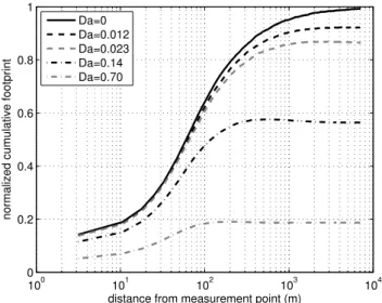
Da=0 Da=0.012 Da=0.023 Da=0.14 Da=0.70
Fig. 1.Example of cumulative flux footprints for inert and reac-tive gases as calculated by the SLTC-model for height of 1.5 times the canopy height. The cumulative footprint of the inert compound (Da = 0) approaches unity while the others are affected by the chem-ical degradation.
In order to estimate the effect of the chemical degradation on the fluxes we give each air parcel in the model an initial concentration valueφ= 1 at the time of release. This concen-tration is then decreased at each time-step as
φk=φk−1exp −1tτc (9)
whereφk is the concentration at the time stepk,φk−1 the
concentration in the previous time step, and1t is the length of the time step. We also consider the emission source to be horizontally homogenous,E(zs), depending only on height,
zs. The flux of a reactive compound at a height zm is thus given by
F (zm)= 1
N N
X
i=1
ni
X
j=1 wij
wij
φ RijE (zs) (10)
whereRijdenotes the path the air parcel has traveled before interception. Integration horizontally to infinity does yield values lower than unity, depending on the chemical lifetime and travel time and path of air parcels. Normalization of the Eq. (10) by dividing with source strength yields an expres-sion to calculate theF/Eratio with our model.
A cumulative footprint function for inert compound and for compounds with different chemical lifetimes is presented in Fig. 1. From this figure one can see how the cumulative footprint of the inert compound approaches unity while those for reactive compounds do not. The asymptotic value of the cumulative footprint is thus the ratio of the flux to the primary emission.
As the parameters in the model are represented in unitless normalized form, the chemical lifetime is also presented in the model as
τcN=u∗τc
h (11)
which is the inverse of the Damk¨ohler number calculated at the height of the canopy top,h. Thus we introduce canopy-top Damk¨ohler number as
Dah= 1
τN
c
= h
u∗τc
. (12)
Damk¨ohler number for a specific measurement height can obtained be from this by
Da=znDah (13)
whereznis the measurement height normalized with canopy height (zn=z/ h).
3 Measurements of oxidants during HUMPPA – COPEC – 2010
The measurements of oxidants used to calculate the chemi-cal lifetimes of VOCs were conducted at SMEAR II research station in Hyyti¨al¨a, Finland as part of the HUMPPA-COPEC-2010 measurement campaign. A detailed description of the measurement campaign has been given by Williams et al. (2011) while the measurement station has been described by Hari and Kulmala (2005). Below we give a short descrip-tion of the measurements utilized in this study.
3.1 Hydroxyl radical concentration
Our measurement of hydroxyl radical (OH) relies on the de-tection of isotopically labeled sulfuric acid with the Chem-ical Ionization Mass Spectrometer (CIMS) This technique is discussed by Eisele and Tanner (1991, 1993), Tanner et al. (1997), and Pet¨aj¨a et al. (2009) in more detail. An impor-tant note on the method that needs to be kept in mind is that we do not measure OH directly, but only infer the ambient OH concentration looking into how much of the isotopically labeled 34SO2 is converted to isotopically labeled sulfuric
acid with a constant reaction time. During the HUMPPA-COPEC campaign (Williams et al. 2011) we compared the CIMS method with a Laser induced fluorescence (LiF) de-tection of OH (Faloona et al. 2004) and the agreement was excellent, with a slope of 1.05 based on side-by-side mea-surements (H. Harder, personal communication, 2011). 3.2 Nitrate radical concentration
Nitrate radical (NO3) was measured at night by
−0.50 0 0.5 1 0.5
1 1.5
z / h
A
−0.50 0 0.5 1
0.5 1 1.5
B
−0.50 0 0.5 1
0.5 1 1.5
C
Dah=0 Dah=0.0078 Dah=0.016 Dah=0.093 Dah=0.47
−0.50 0 0.5 1
0.5 1 1.5
D
z / h
−0.50 0 0.5 1
0.5 1 1.5
E
F / E −0.5 0 0.5 1
0 0.5 1 1.5
F
Fig. 2.Flux-to-surface-exchange (F/E) ratio profiles. The source height, represented by the solid black line, is at the ground level in Panels
(A)–(C)and at the displacement height in Panels(D)–(F). In Panels(B)and(E)the vertical profile of oxidation rate is constant. In Panels
(A)and(D)the oxidation rate below the displacement height is four times faster than above that. In Panels(C)and(F)the oxidation rate
below displacement height is one-fourth of that above displacement height. The canopy-top Damk¨ohler refers to the above canopy chemical lifetime in all Panels. The dashed black line represents the foliage distribution.
before sunset, around 23:00 LT, and stopped 1 h after sun-rise, around 04:00 LT. The two-channel instrument, which sampled NO3 and the sum of NO3 plus N2O5 was located
at the top of a∼20 m tower, i.e. approximately at canopy height. The horizontal distance to the nearest tree-top was about 10 meters. The accuracy of the measurements, con-sidering errors in the cross sections of NO3, inlet and
fil-ter losses of NO3and variability in the zero measurements,
was about 20 %, with a limit of detection of about 1 pptv (2×10⁷molecule cm−3). During the entire campaign both
NO3and N2O5were below the detection limit. The low NO3
mixing ratios were a result of a low NO3 production term,
average nighttime NO2 and O3 being about 350 pptv and
40 ppbv, respectively, resulting in an average NO3
produc-tion rate of 1×10⁻²pptv s−1. The average loss rate for NO3
due to reaction withα-pinene, β-pinene and 3-carene was about 0.03 s−1 with approximate maximum and minimum values on individual nights of 0.07 s−1and 0.01 s−1, respec-tively. When combined with the lowest nighttime reactivity (1×10²s−1) this results in a steady state NO3mixing ratio of
1 pptv only.
3.3 Ozone concentration
Ozone (O3) was measured during HUMPPA COPEC-2010
campaign from the 73 m mast of the SMEAR II at different heights. For characteristic values, mean values of 30 min av-erages at 16.8 m height were used in the study. The O3
mix-ing ratio was determined usmix-ing a Thermo Environment model TEI-49 instrument relying on ultra-violet absorption.
4 Results and discussion
4.1 Oxidation profile and emission height
Figure 2 represents flux-to-surface-exchange ratio (F/E) profiles in hydrostatically neutral stratification, for canopy density and shape representing a typical Scots pine forest. In middle panels (b and e) the chemical lifetime is verti-cally constant representing a constant profile of oxidation rate while the left side panels (a and d) represent the case where the oxidation rate below canopy is four times faster than above the canopy. This could be due to e.g. higher NO3
concentrations in the shaded canopy environment (Forkel et al., 2006). In the right side panels (c and f) the chemical lifetime below the displacement height is four times longer, corresponding e.g. to a case where the OH level in shaded below-canopy environment is lower than above canopy. This type of OH profile was also experimentally observed.
−0.50 0 0.5 1 0.5
1 1.5
z / h
A
−0.50 0 0.5 1
0.5 1 1.5
B
−0.50 0 0.5 1
0.5 1 1.5
C
Dah=0 Dah=0.0078 Dah=0.016 Dah=0.093 Dah=0.47
−0.50 0 0.5 1
0.5 1 1.5
D
z / h
−0.50 0 0.5 1
0.5 1 1.5
E
F / E
−0.50 0 0.5 1
0.5 1 1.5
F
Fig. 3.Effect of canopy density on flux-to-surface-exchange (F/E) ratio. The source height, represented by the solid black line, is at the
ground level in Panels(A)–(C)and at the displacement height in Panels(D)–(F). In Panels(B)and(E)the canopy density corresponds to
that in SMEAR II and used also in Fig. 2. In Panels(A)and(D)the canopy density in half of that in Panels(B)and(E), and in Panels(C)
and(F)the canopy density is double of that in Panels(B)and(E). The canopy-top Damk¨ohler refers to the above canopy chemical lifetime
in all Panels. The dashed black line represents the foliage distribution.
by the oxidant levels also below the source level. In panels d–f we can observe negativeF/E values for chemically re-active cases below the source height, due to the downward fluxes caused by the chemical sink. In the end the oxida-tion rates below source level do have an effect on the above canopy fluxes as the air parcels, which have traveled below source level prior to crossing the observation level above the canopy, have been exposed to the oxidant level below the source level.
TheF/Eprofiles obtained (Fig. 2) are similar as the ones presented earlier by Rinne et al. (2007). However, whereas they presented their results for a specific friction velocity and canopy height we present them in normalized, dimensionless forms as calculated by the SLTC model and show the chem-ical lifetime as Damk¨ohler number at the canopy-top (Dah), as given by Eq. (12). Heights above the surface are relative to the canopy height. This will enable a wider utilization of these results. As the model scales linearly with the friction velocity, one can obtain chemical lifetimes using Eq. (12). If, for example, we consider a compound with chemical a lifetime of 30 minutes emitted from the forest canopy with a height of 18 m and the friction velocity is 0.5 m s−1, the canopy-top Damk¨ohler number is 0.02. If the flux measure-ment height is 22 m the corresponding Damk¨ohler number is 0.024. From Figure 2 we can observe that the fluxes above canopy are significantly reduced already at Damk¨ohler num-bers well below unity. For example in the case of vertically constant chemical lifetime and source at the displacement
−0.50 0 0.5 1 0.2
0.4 0.6 0.8 1 1.2 1.4 1.6
A
F / E
z / h
−0.50 0 0.5 1
0.2 0.4 0.6 0.8 1 1.2 1.4 1.6
F / E B
Da h=0 Da
h=0.0078
Da
h=0.016
Da
h=0.093
Da
h=0.47
Fig. 4.The flux-to-surface-exchange (F/E) ratio profiles calculated using foliage distribution (dashed black line) typical for spruce for-est. The vertical profile of oxidation rate is constant and the source
is either at the ground level (PanelA) or at the height corresponding
to the displacement height of the Scots pine forest.
weight the first crossing gets compared to the later ones, lead-ing to shorter effective transport time.
4.2 Canopy density and structure
The canopy can increase the chemical loss by hindering transport and thus prolonging the transport time, in addition to affecting the lifetimes of VOCs by influencing the con-centrations of oxidants. Keeping the vertical oxidation pro-file constant we investigated the effect of (i) halving or dou-bling canopy density of a Scots pine type forest at SMEAR II (Fig. 3) and (ii) changing the canopy shape from Scots pine to spruce (Fig. 4) The canopy density exerts the expected influence on the F/E profiles in the case with the source at the ground level. The increase in the canopy density re-duces the turbulence below the canopy and thus the transport time from the ground source to above canopy levels increase. This leads to increased flux degradation above the canopy, as there is more time for oxidation. Interestingly, theF/E pro-file in the case with the source at the displacement height seems to be rather insensitive to the canopy density. Obvi-ously the increase in the canopy density reduces the transport downwards from the source level as well as upwards trans-port. Thus it seems that these two effects counterbalance each other and the net effect of canopy density to theF/Eprofiles when the source is at the displacement height is minimal. We must remind here that in this modeling exercise the oxidant profiles were kept constant in spite of changes in canopy den-sity. I reality the increase in canopy density would be likely to reduce the below canopy levels of OH and ozone though shading and providing more surface to deposition. Thus
in-0.3
0.4
0.5
0.6
0.7
0.8
0.9
1 1
h/L
Da
h
F/E at z/h=1.5
−0.2 −0.1 0 0.1 0.2
0 0.05 0.1 0.15 0.2 0.25 0.3
Fig. 5.Effect of stability on the flux-to-surface-exchange (F/E)
ra-tio at the height where measurement height (z) ratio to the canopy
height (h) is 1.5. On x-axis is the inverse of the Obukhov length
(L) normalized with canopy height (h) and on y-axis is the
canopy-top Damk¨ohler number. The numbers on curves refer to flux-to-emission ratios.
creased canopy density may even increase the above-canopy
F/Eratio for reactive compounds emitted from the canopy. TheF/Eprofiles for spruce forest (Fig. 4) are quite simi-lar than for the canopy structure of pine forest (Fig. 3, panel b and e) However, as we choose to have the canopy source at the same height as in the case for Scots pine to ease the comparison between these two, this emission height may be somewhat artificial as for spruce most of the needle biomass is at lower height.
By using the F/E profiles shown in Fig. 2, 3 and 4 we can assess the importance of below canopy chemical pro-cessing to the above canopy one. The degradation below and within canopy is given by 1−F /E(h) whereas the degrada-tion between canopy top and measurement height is given asF/E(h)−F/E(zm). If we set the measurement height to 1.5×h, which is a typical flux measurement height, we see that from 50 % up to over 90 % of the chemical degradation occurs within and below canopy. Even when the source is within the canopy 50 % to well over 80 % of the degradation can occur within and below canopy.
4.3 Hydrostatic stability
All the results discussed above are calculated for hydrostati-cally neutral stratification. In Fig. 5 the effect of stratification on theF/Evalues at the height of 1.5 h is represented. The stability is presented as Obukhov length
L= − u
∗3θ v
κgw′θ′ v
s
whereθv is virtual potential temperature,κ is von K´arm´an
constant, and subscript s refers to surface value (Obukhov, 1971), normalized with canopy height (h/L). The stability range in the figure (−0.25< h/L <0.25) ranges from mod-erately unstable to modmod-erately stable, as an example for canopy height of 15 m fromL= −60 m to L=60 m. Not surprisingly, the normalized fluxes for a given normalized chemical lifetimes are lower in the stable than in the unsta-ble stratification. However, the direct effect of the stability is small compared to that of Dah, i.e. friction velocity and chemical lifetime. If, for example we consider a compound with chemical lifetime corresponding to top-of-the-canopy Damk¨ohler number of 0.1 we find that the flux is reduced by 38 % in neutral case, 32 % whenh/L= −0.25 (forh=15 m,
L= −60) and 45 % whenh/L=0.25, when all other param-eters, including friction velocity are kept constant. We can see from Eq. (14) that this implies that only buoyancy flux is varying in this case. However, as in reality stability exerts a strong control on the turbulence, it has an indirect effect on the flux profiles via the friction velocity.
One must note that in reality, especially in dense canopies, the stability below the canopy can be the opposite to the sta-bility above the canopy. This can greatly modify the transport times inside tha canopy and can have a strong effect espe-cially on theF/E ratios of those compounds emitted from forest floor.
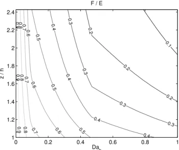
If we neglect the direct effect of stability, to a first approx-imation, we can draw a relation between flux degradation at certain height, friction velocity, and chemical lifetime of a compound. In Fig. 6 is an example for such a relation for source of reactive compound in the canopy and constant ox-idation rate profile. The x-axis shows the top-of-the-canopy Damk¨ohler number, function of friction velocity and chemi-cal lifetime, and the y-axis the height normalized by dividing with the canopy height. The isolines indicateF/Evalues de-termined from profiles shown in Fig. 2, panel e by interpola-tion. We have derived these for normalized chemical lifetime ranges we have the original SLTC runs for and for all the pine canopy densities and oxidation rate profiles (Supplementary material).
4.4 Case study: BVOC fluxes and
HUMPPA-COPEC-2010 oxidant measurements
Using the data used to generate Fig. 6 as a lookup table we can assess the importance of the chemical degradation in dif-ferent conditions. As an example we chose three compounds typically emitted by boreal forests. First one is isoprene, the globally dominant biogenic volatile organic compound (Guenther et al., 1995); the second isα-pinene, the dominant monoterpene in the ecosystem scale emission from Scots pine forests such as Hyyti¨al¨a (Rinne et al., 2000; R¨ais¨anen et al., 2009). These two have typical daytime atmospheric lifetimes of about half an hour in summertime conditions in Hyyti¨al¨a. The third compound isβ-caryophyllene, a typical
0.1
0.2
0.2
0.2 0.3
0.3
0.3
0.3
0.4
0.4
0.4
0.4
0.5
0.5
0.5
0.6
0.6
0.6
0.7
0.7
0.7
0.8
0.8
0.8
0.9
0.9
0.9
111
Dah
z / h
F / E
0 0.2 0.4 0.6 0.8 1
1 1.2 1.4 1.6 1.8 2 2.2 2.4
Fig. 6. Flux-to-surface-exchange (F/E) ratio as a function of
canopy-top Damk¨ohler number and ratio of measurement height (z)
to the canopy height (h). This is a visualization of the look-up table
(Supplementary material).
sesquiterpene compound emitted by pine trees (e.g. Hakola et al., 2006). It is more reactive than isoprene orα-pinene with a daytime lifetime in summertime Hyyti¨al¨a conditions below two minutes. By using typical diurnal cycles of the three oxidants and friction velocity (Fig. 7) and their reac-tion rate constants (Table 2) we can calculate the diurnal cycle of each compounds lifetime (Eq. 4). The diurnal cy-cles of friction velocity, ozone and hydroxyl radical con-centrations are hourly medians measured during HUMPPA-COPEC-2010 campaign (Williams et al., 2011) conducted in SMEAR II research station (Hari and Kulmala, 2005) in July-August 2010, as described above. The effect of stability was ignored for simplicity. During the HUMPPA-COPEC-2010 the daytime medianh/L= −0.1 and night time median h/L=0.25. Also nitrate radical concentrations were measured; however, since they were below detection limit we used cal-culated value of 2.5×10⁷molecules cm−3(1 pptv) at night (22:00–04:00) and zero during daytime.
The relative importance of the three oxidants in the chem-ical degradation on the three VOCs at hand can be seen in Table 3, in which we present oxidative capacities,R, of the three oxidants against VOCs. The oxidative capacities are calculated as
RoxX =kX,ox[ox] (15)
Table 2.Reaction coefficients of isoprene,α-pinene andβ-caryophyllene against OH, O3and NO3. Reaction coefficients for isoprene and
α-pinene from Atkinson (1994) and those forβ-caryophyllene from Shu and Atkinson (1995).
OH cm3molecule−1s−1 O3cm3molecule−1s−1 NO3cm3molecule−1s−1
isoprene 10.1×10⁻¹¹ 1.28×10⁻¹⁷ 6.78×10⁻¹³
α−pinene 5.37×10⁻¹¹ 8.66×10⁻¹⁷ 6.16×10⁻¹²
β−caryophyllene 2.00×10⁻¹⁰ 1.16×10⁻¹⁴ 1.90×10⁻¹¹
Table 3.Oxidative capacities of OH, O3and NO3to isoprene,α-pinene, andβ-caryophyllene.1% is the proportion to the uncertainty to the total oxidative capacity of given VOC.
Day
ROH, s−1 1% RO3, s
−1 1% R
NO3, s
−1 1% R
Total
Isoprene 1.1±0.4×10⁻⁴ 36 1.21±0.03×10⁻⁵ 0.3 0 – 1.2±0.4×10⁻⁴
α-pinene 6±2×10⁻⁵ 17 8.2±0.2×10⁻⁵ 2 0 – 1.4±0.2×10⁻⁴
β-caryophyllene 2.2±0.9×10⁻⁴ 0.8 1.10±0.03×10⁻² 3 0 – 1.1±0.3×10⁻²
Night
Isoprene 3±1×10⁻⁵ 21 9.9±0.3×10⁻⁶ 0.6 1.7±1.7×10⁻⁵ 30 7±2×10⁻⁵
α-pinene 1.5±0.6×10⁻⁵ 2 6.7±0.2×10⁻⁵ 0.9 1.7±1.7×10⁻⁴ 67 2.5±1.6×10⁻⁴
β-caryophyllene 6±2×10⁻⁵ 0.2 9.0±0.3×10⁻³ 3 5±5×10⁻⁴ 5 9.5±0.6×10⁻³
6 12 18
0 0.5 1
time [h] u *
[m s
−1]
6 12 18
0 5 10
x 105
time [h]
OH [cm
−3 ]
6 12 18
0 5 10
x 1011
time [h] O 3
[cm
−3]
6 12 18
0 1 2 3x 10
7
time [h]
NO
3
[cm
−3 ]
Fig. 7. Typical diurnal cycles of friction velocity, OH, O3, and
NO3, as derived from measurements during
HUMPPA-COPEC-2010 campaign.
from the table. First, even at these low calculated nighttime NO3levels the nitrate radical dominates theα-pinene
oxida-tion at night. Second, the low observed levels of OH at night are still sufficient to account for a half of nighttime isoprene oxidation. Also presented in the Table 3 are the estimated uncertainties of oxidative capacities due to the uncertain-ties of oxidant measurements (1O3=1 ppb, 1OH = 40%, 1NO3=1 ppt). We can see from the Table 3 that largest
un-certainties arise from the unun-certainties of OH in the case of daytime isoprene oxidation and NO3in the case of nighttime α-pinene oxidation
In order to use the look-up table (see Supplement) we cal-culated the diurnal cycle of the canopy-top Damk¨ohler num-ber (Dah) for each VOC by using the diurnal cycle of their chemical lifetime (Eq. 4), the diurnal cycle of the friction ve-locity, and Eq. (11). The canopy height was set to 18 m. The flux-to-emission ratio was then retrieved from the look-up table for VOC flux measurement height used in SMEAR II (22 m = 1.2×h).
6 12 18 0
0.2 0.4 0.6 0.8 1
ground source
F / E
6 12 18
0 0.2 0.4 0.6 0.8 1
time [h]
F / E
canopy source
isoprene
α−pinene
β−caryophyllene
Fig. 8.Diurnal cycle of the flux-to-surface-exchange (F/E) ratios
of isoprene, α-pinene andβ-caryophyllene for conditions during
HUMPPA-COPEC-2010 campaign.
calculated the aα-pinene emissions using median diurnal cy-cle of temperatures observed during HUMPPA-COPEC cam-paign with emission algorithm by Guenther et al. (1993)
E=E30exp β T −30◦C (16)
whereE30is the emission standardized to 30◦C temperature, βis the temperature sensitivity of the emission, andT is the temperature. For temperature sensitivity of monoterpenes we used value ofβ=0.09◦C−1. After emission calculated for
each hour was multiplied by correspondingF/Eratio we fit-ted the temperature against flux obtained to yield theβvalue for the flux. The temperature dependence obtained from the fluxes wasβ=0.098◦C−1andβ=0.100◦C−1 for canopy and ground source, respectively. Thus a slightly steeper tem-perature dependence of fluxes than that of primary emission is observed
The chemical degradation affects the fluxes of β -caryophyllene even more as itsF/E ratio is below 0.4 for ground source and about 0.5 for canopy source during the
daytime and falls below 0.2 for groud source and below 0.4 for canopy source during night. Thus the emission of this highly reactive compound is seriously underestimated by the above canopy fluxes. If we use Eq. (16) withβ=0.18◦C−1 (Hakola et al., 2006) to calculate the surface emission of
β-caryophyllene, the temperature dependence of fluxes be-comes β=0.19◦C−1 and β=0.20◦C−1 for canopy and ground source, respectively. As the current development in online mass spectrometry enables the flux measurements of the highly reactive sesquiterpenes (M¨uller et al., 2010; Ru-uskanen et al., 2011) it is of great importance to better un-derstand the processes linking the measured above canopy fluxes to the primary emission of reactive compounds.
5 Conclusions
We have used a stochastic Lagrangian transport model with simplified chemical degradation to estimate the effect of chemistry on ratio of the above canopy fluxes and primary emission. The flux degradation was mostly dependent on the chemical lifetime of the compound and on the friction veloc-ity as the Damk¨ohler number depends on these parameters. Stability as given by the Obukhov-length had a smaller direct effect but it affects the flux-to-surface-exchange (F/E) ratio also via its effect on turbulence intensity. The degradation was stronger for emission from the ground level than from the emission from the canopy, due to longer time required for transport to the above canopy atmosphere.
The oxidant profile had a significant effect on theF/E ra-tio. In the case with higher oxidation rate below canopy the fluxes were degraded more than in the case with constant ox-idation rate. This was case also when the reactive compound was emitted from the canopy. As 50 % or more of the flux degradation occurs below the canopy, the better characteri-zation of the below-canopy turbulent transport and oxidant profiles is essential for understanding the fluxes of reactive compounds. The canopy density had a significant effect only when the emission occurred in the ground level.
interpreting flux directly as emission can lead to artificial cor-relations between emission and these environmental param-eters.
There are uncertainties of the various parts of the ap-proach. Many of these have to do with the below-canopy atmosphere. First the below canopy turbulent flow is not well characterized as shown by reported discrepancies be-tween observations and models. Also the basal layer, as the soil emissions must traverse it, should be better character-ized. While ozone concentration profiles within and below many plant canopies have been measured, the profiles or even above and below canopy concentrations of hydroxyl and ni-trate radical are often lacking. Furthermore the so-called seg-regation effect, which can affect the calculated chemical life times, is hardly well known. These all call for further studies of the interactions between chemistry and turbulent transport above and within plant canopies.
Supplementary material related to this article is
available online at: http://www.atmos-chem-phys.net/12/ 4843/2012/acp-12-4843-2012-supplement.zip.
Acknowledgements. Funding from the Academy of Finland (139656, 1118615, 120434, 125238), Finnish Centre of Excellence funded by Academy of Finland (141135), and European Research Council (227463-ATMNUCLE) is gratefully acknowledged. Help of the SMEAR II personnel (J. Levula, T. Pohja, V. Hiltunen, H. Laakso) during the field campaign is gratefully acknowledged.
Edited by: D. Heard
References
Atkinson, R.: Gas-phase tropospheric chemistry of organic com-pounds, J. Phys. Chem. Ref. Data. Monogr., 2, 216 pp.,, 1994. Boy, M., Sogachev, A., Lauros, J., Zhou, L., Guenther, A., and
Smolander, S.: SOSA – a new model to simulate the concen-trations of organic vapours and sulphuric acid inside the ABL – Part 1: Model description and initial evaluation, Atmos. Chem. Phys., 11, 43–51, doi:10.5194/acp-11-43-2011, 2011.
Ciccioli, P., Brancaleoni, E., Frattoni, M., Di Palo, V., Valentini, R., Tirone, G., Seufert, G., Bertin, N., Hansen, U., Csiky, O., Lenz, R., and Sharma, M.: Emission of reactive terpene compounds from orange orchards and their removal by within-canopy pro-cesses. J. Geophys. Res., 104, 8077–8094, 1999
Crowley, J.N., Schuster, G., Pouvesle, N., Parchatka, U., Fischer, H., Bonn, B., Bingemer, H., and Lelieveld, J.: Nocturnal nitro-gen oxides at a rural mountain site in south-western Germany, Atmos. Chem. Phys., 10, 2795–2812, doi:10.5194/acp-10-2795-2010, 2010.
Damk¨ohler, G.: Der Einfluss der Turbulenz auf die Flam-mengeschwindigkeit in Gasgemischen, Zeitschrift f¨ur Electro-chemie und Angewandte Physikalische Chemie, 46, 601–626, 1940.
Eisele, F. and Tanner, D.: Ion-assisted tropospheric OH measure-ments, J. Geophys. Res., 96, 9295–9308, 1991.
Eisele, F. and Tanner, D.: Measurement of the gas phase concen-tration of H2SO4 and methane sulfonic acid and estimates of H2SO4 production and loss in the atmosphere, J. Geophys. Res., 98, 9001–9010, 1993.
Faloona, I. C., Tan, D., Lesher, R. L., Hazen, N. L., Frame, C. L., Simpas, J. B., Harder, H., Martinez, M., Di Carlo, P., Ren, X., and Brune, W. H.: A Laser-induced Fluorescence Instrument for
detecting tropospheric OH and HO2: characteristics and
calibra-tion, J. Atmos. Chem. 47, 139–167, 2004
Forkel, R., Klemm, O., Graus, M., Rappengluck, B., Stockwell, W. R., Grabmer, W., Held, A., Hansel, A., and Steinbrecher, R.: Trace gas exchange and gas phase chemistry in a Norway spruce forest: A study with a coupled 1-dimensional canopy at-mospheric chemistry emission model, Atmos. Environ., 40, Sup-plement 1, S28–S42, 2006.
Fowler, D., Pilegaard, K., Sutton, M. A., Ambus, P., Raivonen, M., Duyzer, J., Simpson, D., Fagerli, H., Fuzzi, S., Schjoerring, J. K., Granier, C., Neftel, A., Isaksen, I. S. A., Laj, P., Maione, M., Monks, P. S., Burkhardt, J., Daemmgen, U., Neirynck, J., Per-sonne, E., Wichink-Kruit, R., Butterbach-Bahl, K., Flechard, C., Tuovinen, J. P., Coyle, M., Gerosa, G., Loubet, B., Altimir, N., Gruenhage, L., Ammann, C., Cieslik, S., Paoletti, E., Mikkelsen, T. N., Ro-Poulsen, H., Cellier, P., Cape, J. N., Horv´ath, L.,
Loreto, F., Niinemets, ¨U., Palmer, P. I., Rinne, J., Misztal, P.,
Nemitz, E., Nilsson, D., Pryor, S., Gallagher, M. W., Vesala, T., Skiba, U., Br¨ueggemann, N., Zechmeister-Boltenstern, S., Williams, J., O’Dowd, C., Facchini, M. C., de Leeuw, G., Floss-man, A., Chaumerliaco, N., and ErisFloss-man, J. W.: Atmospheric Composition Change: Ecosystems – Atmosphere interactions. Atmos. Environ., 43, 5193–5267, 2009
Guenther, A., Zimmermann, P., Harley, P., Monson, R., and Fall, R.: Isoprene and monoterpene emission rate variability: Model evaluation and sensitivity analysis, J. Geophys. Res., 98, 12609– 12617, 1993.
Guenther, A., Hewitt, C. N., Erickson, D., Fall, R., Geron, C., Graedel, T., Harley, P., Klinger, L., Lerdau, M., McKay W. A., Pierce T., Scholes, B., Steinbrecher, R., Tallamraju, R., Taylor, J., and Zimmerman, P.: A global model of natural volatile or-ganic compound emissions. J. Geophys. Res., 100, 8873–8892, 1995
Hakola, H., Tarvainen, V., B¨ack, J., Ranta, H., Bonn, B., Rinne, J., and Kulmala, M.: Seasonal variation of mono- and sesquiterpene emission rates of Scots pine. Biogeosci., 3, 93–101, 2006. Hari, P. and Kulmala, M.: Station for measuring ecosystem
atmo-sphere relations (SMEAR II), Boreal Environ. Res., 10, 315–322, 2005.
H¨ortnagl, L., Bamberger, I., Graus, M. Ruuskanen, T. M. Schnitzhofer, R., M¨uller, M. Hansel, A., and Wohlfahrt G.: Bi-otic, abiBi-otic, and management controls on methanol exchange above a temperate mountain grassland, J. Geophys. Res., 116, G03021, doi:10.1029/2011JG001641, 2011.
USA, 183–206, 2009.
Launiainen, S., Rinne, J., Pumpanen, J., Kulmala, L., Kolari, P., Keronen, P., Siivola, E., Pohja, T., Hari, P., and Vesala, T.: Eddy-covariance measurements of CO2 and sensible and latent heat fluxes during a full year in a boreal pine forest trunk-space. Bo-real Environ. Res., 10, 569–588, 2005
Markkanen, T., Rannik, ¨U., Marcolla, B., Cescatti, A. and Vesala,
T.: Footprints and fetches for fluxes over forest canopies with varying structure and density, Bound.-Layer Meteorol., 106, 437–459, 2003.
Massman, W. J.: An Analytical one-dimensional model of momen-tum transfer by vegetation of arbitrary structure, Bound.-Layer Meteorol., 83, 407–421, 1997.
Massman, W. J. and Weil, J. C.: An analytical one-dimensional second-order closure model of turbulence statistics and the La-grangian time scale within and above plant canopies of arbitrary structure, Bound.-Layer Meteorol. 91, 81–107, 1999.
M¨uller, M., Graus, M., Ruuskanen, T. M., Schnitzhofer, R., Bam-berger, I., Kaser, L., Titzmann, T., H¨ortnagl, L., Wohlfahrt, G., Karl, T., and Hansel, A.: First eddy covariance flux mea-surements by PTR-TOF, Atmos. Meas. Tech., 3, 387–395, doi:10.5194/amt-3-387-2010, 2010.
Obukhov, A. M.: Turbulence in an atmosphere with a non-uniform temperature. Bound.-Layer Meteorol. 2, 7–29, 1971
Pet¨aj¨a, T., Mauldin III, R. L., Kosciuch, E., McGrath, J., Nieminen, T., Adamov, A., Kotiaho, T., and Kulmala, M.: Sulfuric acid and OH concentrations in a boreal forest site, Atmos. Chem. Phys. 9, 7435–7448, doi:10.5194/acp-9-7435-2009, 2009
R¨ais¨anen, T., Ryypp¨o, A., and Kellom¨aki, S.: Monoterpene emis-sion of a boreal Scots pine (Pinus sylvestris L.) forest, Agric. For. Meteorol., 149, 808–819, 2009.
Rannik, ¨U., Aubinet, M., Kurbanmuradov, O., Sabelfeld, K. K.,
Markkanen, T., and Vesala, T.: Footprint analysis for measure-ments over a heterogeneous forest. Bound.-Layer Meteorol., 97, 137-166, 2001.
Rannik, ¨U., Markkanen, T., Raittila, J., Hari, P., and Vesala, T.:
Tur-bulence statistics inside and over forest: Influence on footprint prediction, Bound.-Layer Meteorol., 109, 163–189, 2003.
Rannik, ¨U., Sogachev, A., Foken, T., G¨ockede, M., Kljun, N.,
Leclerc, M. Y., and Vesala, T.: Footprint Analysis, edited by: Aubinet, M., Vesala, T., Papale, D., in: Eddy Covariance Hand-book, Springer, 211–261, 2012.
Rinne, J., Hakola, H., Laurila, T., and Rannik, ¨U.: Canopy scale
monoterpene emissions of Pinus sylvestris dominated forests, Atmos. Environ., 34, 1099–1107, 2000.
Rinne, H. J. I., Guenther, A. B., Greenberg, J. P., and Harley, P. C.: Isoprene and monoterpene fluxes measured above Amazo-nian rainforest and their dependence on light and temperature, Atmos. Environ., 36, 2421–2426, 2002.
Rinne, J., Taipale, R., Markkanen, T., Ruuskanen, T. M., Hell´en, H., Kajos, M. K., Vesala, T., and Kulmala, M.: Hydrocarbon fluxes above a Scots pine forest canopy: measurements and mod-eling, Atmos. Chem. Phys., 7, 3361–3372, doi:10.5194/acp-7-3361-2007, 2007.
Rinne, J., B¨ack J., and Hakola, H.: Biogenic volatile organic com-pound emissions from Eurasian taiga: Current knowledge and future directions, Boreal Environ. Res., 14, 807–826, 2009 Ruuskanen, T. M., M¨uller, M., Schnitzhofer, R., Karl, T., Graus, M.,
Bamberger, I., H¨ortnagl, L., Brilli, F., Wohlfahrt, G., and Hansel, A.: Eddy covariance VOC emission and deposition fluxes above grassland using PTR-TOF, Atmos. Chem. Phys., 11, 611–625, doi:10.5194/acp-11-611-2011, 2011.
Shu, Y. and Atkinson, R: Atmospheric lifetimes and fates of a series of sesquiterpenes. J. Geophys. Res., 100, 7275–7281, 1995. Strong, C., Fuentes, J. D., and Baldocchi, D.: Reactive hydrocarbon
footprints during canopy senescence, Agric. For. Meteorol., 127, 159–173, 2004.
Stull, R. B.: An Introduction to Boundary Layer Meteorology. Kluwer Academic Publishers, Dortrecht, The Netherlands, 666 pp., 1988.
Taipale, R., Kajos, M. K., Patokoski, J., Rantala, P., Ruuskanen, T. M., and Rinne, J.: Role of de novo biosynthesis in ecosys-tem scale monoterpene emissions from a boreal Scots pine forest, Biogeosciences, 8, 2247–2255, doi:10.5194/bg-8-2247-2011, 2011.
Tanner, D., Jefferson, A., and Eisele, F.: Selected ion chemical ionization mass spectrometric measurement of OH. J. Geophys. Res., 102, 6415–6425, 1997.
Thomson, D. J.: Criteria for the selection of stochastic models of particle trajectories in turbulent flows. J. Fluid. Mech. 180, 529– 556, 1987.
Vesala, T., Kljun, N., Rannik, ¨U., Rinne, J., Sogachev, A.,
Markka-nen, T., Sabelfeld, K., Foken, Th., and Leclerc, M. Y.: Flux and concentration footprint modelling: State of the art. Environ. Poll., 152, 653–666, 2008.