A coupling alternative to reactive transport simulations for long-term prediction of chemical reactions in heterogeneous CO<sub>2</sub> storage systems

(1)

GMDD

7, 6217–6261, 2014

Coupling alternative for reactive transport

M. De Lucia et al.

Title Page

Abstract Introduction

Conclusions References

Tables Figures

◭ ◮

Back Close

Full Screen / Esc

Printer-friendly Version Interactive Discussion

Discussion

P

a

per

|

Discus

sion

P

a

per

|

Discussion

P

a

per

|

Discussion

P

a

per

|

Geosci. Model Dev. Discuss., 7, 6217–6261, 2014 www.geosci-model-dev-discuss.net/7/6217/2014/ doi:10.5194/gmdd-7-6217-2014

This discussion paper is/has been under review for the journal Geoscientific Model Development (GMD). Please refer to the corresponding final paper in GMD if available.

A coupling alternative to reactive

transport simulations for long-term

prediction of chemical reactions in

heterogeneous CO

₂

storage systems

M. De Lucia, T. Kempka, and M. Kühn

GFZ German Research Centre for Geosciences, Sect. 5.3 – Hydrogeology, Telegrafenberg, 14473 Potsdam, Germany

Received: 21 August 2014 – Accepted: 15 September 2014 – Published: 25 September 2014

Correspondence to: M. De Lucia (delucia@gfz-potsdam.de)

(2)

GMDD

7, 6217–6261, 2014

M. De Lucia et al.

Title Page

Tables Figures

◭ ◮

Back Close

Full Screen / Esc

Discussion

P

a

per

|

Discus

sion

P

a

per

|

Discussion

P

a

per

|

Discussion

P

a

per

|

Abstract

Fully-coupled, multi-phase reactive transport simulations of CO2 storage systems can

be approximated by a simplified one-way coupling of hydrodynamics and reactive chemistry. The main characteristics of such systems, and hypotheses underlying the proposed alternative coupling, are (i) that the presence of CO2is the only driving force

5

for chemical reactions and (ii) that its migration in the reservoir is only marginally af-fected by immobilization due to chemical reactions. In the simplified coupling, the expo-sure time to CO2of each element of the hydrodynamic grid is estimated by non-reactive

simulations and the reaction path of one single batch geochemical model is applied to each grid element during its exposure time. In heterogeneous settings, analytical

scal-10

ing relationships provide the dependency of velocity and amount of reactions to poros-ity and gas saturation. The analysis of TOUGHREACT fully coupled reactive transport simulations of CO₂ injection in saline aquifer, inspired to the Ketzin pilot site (Ger-many), both in homogeneous and heterogeneous settings, confirms that the reaction paths predicted by fully coupled simulations in every element of the grid show a high

15

degree of self-similarity. A threshold value for the minimum concentration of dissolved CO2considered chemically active is showed to mitigate the effects of the discrepancy

between dissolved CO2migration in non-reactive and fully coupled simulations. In real

life, the optimal threshold value is unknown and has to be estimated, e.g., by means of 1-D or 2-D simulations, resulting in an uncertainty ultimately due to the process

de-20

(3)

GMDD

7, 6217–6261, 2014

M. De Lucia et al.

Title Page

Tables Figures

◭ ◮

Back Close

Full Screen / Esc

Discussion

P

a

per

|

Discus

sion

P

a

per

|

Discussion

P

a

per

|

Discussion

P

a

per

|

1 Introduction

Long-term, reservoir-scale, multiphase reactive transport simulations in heterogeneous settings are computationally extremely challenging, often forcing to set up oversim-plified models if compared to purely hydrodynamic simulations. Typically, 1-D or 2-D models are preferred wherever symmetry allows for it (e.g., Gaus et al., 2005; White

5

et al., 2005; Audigane et al., 2007; Xu et al., 2010; Beyer et al., 2012); only coarse spatial discretizations are adopted for 3-D models (Nghiem et al., 2004; Kühn et al., 2006; Kühn and Günther, 2007; Zheng et al., 2009). As a result, most studies of re-active transport only consider very simple geometries and homogeneous media, thus disregarding spatial heterogeneities at reservoir scale, which in turn are routinely

con-10

sidered by the usually much more detailed geologic models and pure hydrodynamic reservoir simulations. These oversimplifications concern the chemistry as well, leading to consider only a subset of the potentially reactive minerals. Moreover, the need for sensitivity and uncertainty analysis due to the large amount of uncertain parameters in geochemical simulations (De Lucia et al., 2012; Dethlefsen et al., 2012) cannot be met

15

if the computational effort for one single simulation is too high. The resulting models can be used to highlight qualitative results or to provide rough estimations of the on-going processes at reservoir scale (Gaus et al., 2008, and references therein). To our knowledge, there is no example of fully coupled reactive transport simulations consid-ering complex chemistry on spatial discretizations with a resolution comparable with

20

the one usually adopted for pure hydrodynamic simulations.

However, a number of relevant questions require a rather careful description of reser-voir heterogeneity, or depend on a fine resolution of reserreser-voir features, well beyond the possibility of fully coupled simulators and computationally affordable coarse grids. The migration path in a highly heterogeneous system, for example, heavily affects the

25

(4)

GMDD

7, 6217–6261, 2014

M. De Lucia et al.

Title Page

Tables Figures

◭ ◮

Back Close

Full Screen / Esc

Discussion

P

a

per

|

Discus

sion

P

a

per

|

Discussion

P

a

per

|

Discussion

P

a

per

|

to satisfactorily capture such migration, adding a decisive imprecision to the coarse coupled simulations.

Especially to solve one of these problems, namely the estimation of the long term mineralization at the Ketzin pilot site (Martens et al., 2013), a simplified scheme for cou-pling chemistry and hydrodynamics was introduced (Klein et al., 2013; Kempka et al.,

5

2013b). The purpose of the novel method is to avoid upscaling the simulation grid or applying multi-grid methods, but instead to take advantage of some of the characteris-tics of the modelled processes, by simplifying thecoupling itself.

In CO2storage systems, in fact, relevant mineralization is generally expected to

oc-cur hundreds or thousands years after injection stop (IPCC, 2005), since the slow

kinet-10

ics of the involved reactive chemistry is the typical limiting factor (Marini, 2006; Gaus, 2010). The coupling with hydrodynamic transport of solutes plays only a secondary role under these circumstances. In summary, a typical underground CO2storage system is

expected to display the following characteristics:

1. the time scale of mineral alterations is much larger than that of the hydrodynamic

15

processes, meaning that most relevant chemical alterations are occurring when the system has reached substantial hydrodynamic equilibrium;

2. the major driving force for these alterations is the presence of the injected CO2,

either in a separate, dense phase or dissolved in the formation brine;

3. as consequence of the previous facts, the transport of other reactants is far less

20

relevant with regard to reactions outcome; also, given the high salinity of the tar-geted formation fluids, the presence of other reactants is not a limiting factor for the reactions;

4. the expected mineral reactions do not significantly affect the petrophysical prop-erties of the medium (porosity, permeability) at least until reaching substantial

25

(5)

GMDD

7, 6217–6261, 2014

M. De Lucia et al.

Title Page

Tables Figures

◭ ◮

Back Close

Full Screen / Esc

Discussion

P

a

per

|

Discus

sion

P

a

per

|

Discussion

P

a

per

|

Discussion

P

a

per

|

The resulting coupling approach is described in detail in the next Sect. 2.1, highlighting the major underlying hypotheses for its applicability. Section 3 introduces the case study, with the reference geochemical model, the simulation grid and the general setup of the non-reactive and fully coupled reactive transport simulations performed for the validation. Their respective results are analysed in Sect. 4 aiming at verifying the major

5

hypotheses; and finally a comparison of the outcomes of simplified and full coupling concludes the study.

2 The simplified one-way coupling

2.1 Implementation

The concept of the one-way coupling firstly introduced by Klein et al. (2013) is to

com-10

bine, in a post-processing approach, independent batch geochemical simulations with non-reactive flow simulations, while applying some criterion to at least ensure partial mass balance and thus compensate for the lack of feedback between the modelled pro-cesses. One crucial hypothesis underlying the applicability of the method, as pointed out in the previous section, is that the effects of chemical reactions are small and

be-15

come significant only when the hydraulics of the reservoir have come to a substantial equilibrium, hence not affecting the hydrodynamic behavior of medium and modelled fluids.

In detail, the procedure is constituted by the following steps:

1. from hydrodynamical simulations derive theexposure timeto injected CO2of each

20

grid element, distinguishing between exposure to gaseous or dissolved CO2;

2. compute the characteristic water saturation and concentration of dissolved CO2

during exposure time;

3. one 0-D batch geochemical simulation isanalytically scaled for each element of the hydrodynamic grid, considering heterogeneous porosity and the water/rock

(6)

GMDD

7, 6217–6261, 2014

M. De Lucia et al.

Title Page

Tables Figures

◭ ◮

Back Close

Full Screen / Esc

Discussion

P

a

per

|

Discus

sion

P

a

per

|

Discussion

P

a

per

|

Discussion

P

a

per

|

ratio, which itself depends on gas saturation (insights about the analytical rela-tionship are given in Sect. 2.2);

4. if the element is exposed only to a dissolved CO2concentration, athreshold must

be defined for dissolved CO₂ to be geochemically active. In this case, the miner-alization is limited to the maximum dissolved concentration;

5

5. if the element is exposed only to gaseous CO2, it is assumed that enough CO2

is present in the element to achieve the maximum mineralization without further need for a mass balance;

6. the mineralization in each element is finally summed in time to achieve global mineralization in reservoir.

10

The lack of feedback between hydrodynamics and chemistry is of course the major drawback of this simplified coupling. The absence of direct coupling also does not allow to ensure mass balance between the two processes. These issues therefore permit the application of the method only in case of limited feedbacks not significantly affecting the respective process simulations. However, a control regarding the mass

15

balance has been included into the simplified coupling: in the elements exposed only to dissolved CO₂, the amount of mineralization is limited to the actual amount of CO₂ reaching those elements. This bounding is considered not necessary if a significant saturation of gaseous CO2 is reached in the element, since, given the hypothesis of

small amount of reactions, it is assumed that in such case enough CO₂ is available to

20

reach full mineralization for the given time frame.

The simplified coupling is applied to non-reactive hydrodynamic simulations, where indeed no CO₂is immobilized in precipitating minerals. As a consequence, the spatial extent of the CO2cloud calculated by non-reactive simulations is always equal or larger

than the one predicted if reactive chemistry is considered. This is of course reflected in

25

(7)

GMDD

7, 6217–6261, 2014

M. De Lucia et al.

Title Page

Tables Figures

◭ ◮

Back Close

Full Screen / Esc

Discussion

P

a

per

|

Discus

sion

P

a

per

|

Discussion

P

a

per

|

Discussion

P

a

per

|

Therefore, thefirst main hypothesisneeded for the success of the simplified coupling is that the discrepancy of the CO2migration predicted by the non-reactive simulations

is not too large with respect to the case with active chemistry. It will be shown in the following how the proposed method of defining athreshold on the dissolved CO₂ con-centration “allowed” to activate the chemistry mitigates this issue to a large extent.

5

One major feature integrated in the proposed simplified coupling approach is the treatment of spatial heterogeneity of porosity and of gas saturation in the porous medium, the latter also dynamically variating along the simulation run. These parame-ters namely control speed and total amount of the chemical reactions through the ratio between reactive solution and available mineral surfaces. This scaling can be directly

10

solved by an analytic solution which allows to transform the results of geochemical simulations scaled for a given porosity and water saturation to any other given porosity and saturation. More insights on this matter are given in Sect. 2.2. The gas content, and hence water saturation, and dissolved concentration vary during the simulation and also in particular during the exposure time of grid elements to the injected CO2.

15

By comparison with fully coupled simulations, it can be shown that themaximum gas saturation during exposure time controls the speed of reactions; the maximum con-centration of dissolvedCO2controls the total amount of mineralization in the elements

where no gaseousCO2arrives.

For an initially geochemically homogeneous scenario, the simplified coupling

fore-20

sees the use of one single batch geochemical model which is practically replicated onto all elements of the simulation grid, scaled following the actual local porosity and gas/water saturation ratio. In other words, the simplified coupling assumes that in each element of the simulation grid the reaction path is qualitatively and quantitatively sim-ilar to one single underlying model: we will refer to this property in the following as

25

(8)

GMDD

7, 6217–6261, 2014

M. De Lucia et al.

Title Page

Tables Figures

◭ ◮

Back Close

Full Screen / Esc

Discussion

P

a

per

|

Discus

sion

P

a

per

|

Discussion

P

a

per

|

Discussion

P

a

per

|

The medium considered throughout this study ishomogeneous in terms of volume fractions of reactive minerals: heterogeneity is in the present study only referred to porosity and permeability. In presence of different facies or a spatially heterogeneous distribution of volume fractions, the method can still be applied using as many batch geochemical simulations as there are different facies in the reservoir, then assigning

5

the corresponding chemistry to each element of the hydrodynamic grid. However this possibility has not been explored in the present study.

2.2 The analytical scaling relationship

Klein et al. (2013) introduced the analytical relationships relating the outcome of a sin-gle geochemical simulation, scaled for a given porosity and water saturation, to any

10

other given porosity and saturation. In the following it will be demonstrated that the equations are a direct consequence of the particular form of the kinetic law imple-mented in the models, and of the choice for representing the minerals’ reactive surface and possibly its variation along the simulation.

Consider a reference rock volume V_r. A common rate expression per mass unit of

15

solvent (with dimensions of [mol1+γs−1

kg H₂O−1−γ

]) takes the form (Lasaga, 1998):

r₌k·A_s·(1−Ωα)β·aγ (1)

where k is the kinetic coefficient [mol m2s−1], A_s [m2kg H2O

−1

] is the specific (per mass unit of solvent) reactive surface of the mineral in contact with the solution, Ω

the saturation ratio of the mineral andα,β two fitting parameters; a is the activity of

20

a solute species acting as catalyzer and its exponentγdefines theorder of the kinetic law. The specific reactive surface can be written as:

A_s₌V_m·A_m (2)

whereV_m [m3mineral kg H₂O−1

] is the volume of the mineral in contact with the unit mass of solvent in the considered system andA_m[m2m−3

mineral] the specific reactive

(9)

GMDD

7, 6217–6261, 2014

M. De Lucia et al.

Title Page

Tables Figures

◭ ◮

Back Close

Full Screen / Esc

Discussion

P

a

per

|

Discus

sion

P

a

per

|

Discussion

P

a

per

|

Discussion

P

a

per

|

surface per unit of mineral volume. A_m is a parameter intrinsic to the mineral – e.g. related to grain size. The expression ofV_min terms of porosity and water saturation for the reference rock volumeV_rreads:

V_m₌volume of mineral inVr

mass of solvent inV_r =

V_r·(1−ϕ)·f_m V_r·ρ_H

2O·Sw·ϕ

(3)

whereϕ the porosity,f_m the volume fraction of mineral m referred to all minerals and

5 ρ_H

2O the density (mass of water per unit volume of solution).

The rater, including its dependency on porosity and water saturation, reads then:

r₌k· fm

·(1−ϕ)

ρ_H

2O

·S_w·ϕ

·(1−Ωα)β·aγ (4)

Consider now two distinct rock volumesV₁andV₂with initially equal mineral volume fractions and chemical composition (concentrations) of the reactive solution and diff

er-10

ing only per porosity and saturation, respectivelyϕ₁,S₁andϕ₂,S₂. The rates as seen by the volume unit of solution are:

r₁₌k· fm

·(1−ϕ₁) ρ_H

2O·S1·ϕ1

·(1−Ωα

1)

β_·_aγ

r₂=k·

f_m·(1−ϕ₂) ρ_H

2O·S2·ϕ2

·(1−Ωα

2)

β_·_aγ

(5)

It is not needed to explicitely integrate these equations to compute their respective time

15

(10)

GMDD

7, 6217–6261, 2014

M. De Lucia et al.

Title Page

Tables Figures

◭ ◮

Back Close

Full Screen / Esc

Discussion

P

a

per

|

Discus

sion

P

a

per

|

Discussion

P

a

per

|

Discussion

P

a

per

|

[mol kg H2O

−1

], which is often calledprogress of reaction. We have:

r(t)=dξ

dt =⇒

   

  

V₁:r₁(t₁) =dξ1

dt (t1)

V₂:r₂(t₂) =dξ2

dt (t2)

(6)

Sought are the times t₁ and t₂ at which the reactions in V₁ and V₂ reach the same progress, or ξ₁(t₁)=ξ₂(t₂). Consider time steps ∆t₁₌t₁−t₀ and ∆t₂=t₂−t₀ small 5

enough that the ratesr₁andr₂can be considered constant and the changes in water saturation and porosity become negligible. One can write:

r₁(t₀)≈ ∆ξ ′

∆t₁; r2(t0)≈ ∆ξ′

∆t₂ =⇒∆t2= r₁(t₀)

r₂(t₀)·∆t1 (7)

Substituting Eq. (5) into Eq. (7) and simplifying for thef_m,ρ_H

2Oand theΩterms, which by definition are equal for bothV₁andV₂at the timet₀, we finally obtain:

10

∆t₂₌(1−ϕ1) S₁·ϕ

1

S₂·ϕ₂

(1−ϕ₂)

·∆t₁ (8)

Upon reaching respectivelyt₁ and t₂, the solutions in V₁ andV₂ are again completely equivalent, and so are the (1−Ω) terms, which only depend on activity coefficients and

aqueous concentrations. Hence, the procedure can be repeated, meaning that for any given timet₁inV₁, the same reaction progress is reached inV₂at the timet₂if:

15

t₂₌(1−ϕ1) S₁·ϕ

1

S₂·ϕ₂

(1−ϕ₂)

·t₁ (9)

Furthermore, if∆ξ′is the amount of reaction per unit mass of solvent, the total amount of reactionN in the given rock volume is:

N₁(t₁)=V₁·ρ_H

2O

·ϕ₁·S₁·∆ξ′ (10)

N₂(t₂)=V₂·ρ_H

2O·ϕ2·S2·∆ξ ′

(11)

GMDD

7, 6217–6261, 2014

M. De Lucia et al.

Title Page

Tables Figures

◭ ◮

Back Close

Full Screen / Esc

Discussion

P

a

per

|

Discus

sion

P

a

per

|

Discussion

P

a

per

|

Discussion

P

a

per

|

Dividing the two equations and rearranging, it finally reads:

N₂(t₂)=V2·ϕ2·S2

V₁·ϕ₁·S₁N1(t1) (12)

Equations (9) and (12) are the scaling equations introduced by Klein et al. (2013), given here in a slightly more general form.

Notably, this result holds also for kinetic laws where the total rate is a linear

combina-5

tion of terms of the same form of Eq. (1), and for mixed kinetics/equilibrium simulation as well, since equilibrium is a special case of kinetics where the kinetic constantk is very large. One major assumption still has to be respected, which is that the reactions do not significantly affect the porosityϕand the water saturationS.

Scaling relationship for the TOUGHREACT simulator 10

The TOUGHREACT simulator (Xu et al., 2011) implements the calculation of reactive surfaces canceling out its dependence on water saturation to prevent diverging rates when water saturation is small (Xu et al., 2008, Appendix G, p. 175). Hence, the scaling equations for this simulator read:

   

  

t₂₌(1−ϕ1) ϕ₁

ϕ₂

(1−ϕ

2)

·t₁

N₂(t₂)=V2·ϕ2·S2 V₁·ϕ₁·S₁N1(t1)

(13)

15

3 Validation of the simplified scheme

The procedure for validating the one-way coupling involves the comparison and analy-sis of a case study for which both the simplified coupling approach and the fully coupled reactive transport simulation are applied.

(12)

GMDD

7, 6217–6261, 2014

M. De Lucia et al.

Title Page

Tables Figures

◭ ◮

Back Close

Full Screen / Esc

Discussion

P

a

per

|

Discus

sion

P

a

per

|

Discussion

P

a

per

|

Discussion

P

a

per

|

The case study has been chosen in order to ensure typical conditions for the ap-plication range of the simplified coupling, and is inspired by published models for the Ketzin pilot site (Kempka and Kühn, 2013; Klein et al., 2013). For all simulations the TOUGHREACT/ECO2N (Pruess and Spycher, 2007; Xu et al., 2011) simulator was adopted. However, the simplified coupling is a general method and is independent

5

from the simulator used for the validation.

The influence of spatial heterogeneity, here limited to porosity and permeability, and of the characteristic time scale of reactions relative to the characteristic time scale of CO2migration were also investigated.

3.1 Geochemical model 10

The chemical system chosen for the validation reflects the analyses published by Förster et al. (2010); Norden et al. (2010); Würdemann et al. (2010) and is based on the model for the Ketzin test site published by Klein et al. (2013). The chosen model displays a typical complexity for CO₂storage problems; there is no need and no claim of being an accurate quantitative reference for the site, nor to investigate its plausibility

15

or the quality of the thermodynamic database adopted for the simulations.

The Stuttgart Formation is the target reservoir of the Ketzin pilot site. It is mainly constituted by sand channels and floodplain facies. Reservoir simulations (Kempka and Kühn, 2013) show that the sandy facies receives the major amount of the injected CO2 due to their higher conductivity, and can therefore be retained as the reference

20

facies for investigating the chemical processes.

The rock-forming phases considered reactive are anhydrite, albite, hematite, illite and chlorite, together amounting to 24 % in volume of the rock. The rest of the rock – principally quartz, up to 40 % in volume – is considered inert. Secondary phases in-cluded in the model are kaolinite and the carbonates siderite, magnesite, dolomite and

25

(13)

GMDD

7, 6217–6261, 2014

M. De Lucia et al.

Title Page

Tables Figures

◭ ◮

Back Close

Full Screen / Esc

Discussion

P

a

per

|

Discus

sion

P

a

per

|

Discussion

P

a

per

|

Discussion

P

a

per

|

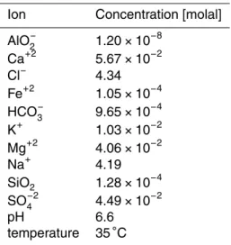
estimation of specific surface areas by Klein et al. (2013). Notably, one order of magni-tude is preserved between the specific reactive surface areas of clay minerals (kaolin-ite, chlorite and illite) and the non-clays. For the initial brine composition the available analyses of Würdemann et al. (2010) have been considered without further refinement besides the concentrations of SiO2and AlO

−

2 which were taken from the re-evaluation

5

performed by Klein et al. (2013).

The batch model, also simulated with TOUGHREACT, is defined as a porous medium of 1 m3volume, represented as one single cubic element in the program. The minerals’ volume fractions listed in Table 2 are assigned to the medium. The rest of pore space not occupied by the brine is assumed filled with CO₂ at an initial pressure of 70 bar,

10

which is an average value derived by the analysis of the hydrodynamic simulations of Kempka and Kühn (2013). The impact of pore pressure was investigated by Klein et al. (2013) by means of batch models with constant pressure, and found negligible with respect to the speed of reactions at least in the range of pressure expected in Ketzin. In the present case the system is closed, and thus the simulation is performed atconstant

15

volumefor the gas phase. The change in porosity and the consommation of water due to reactions, as well as the solubility of H₂O in the gas phase, are negligible in terms of volume change. Hence, the initial pressure governs how much CO2is contained in the

reference volume and therefore available for reactions. The reference simulation is for this reason chosen with an initial porosityϕ₌0.5 and a water saturation ofS_w₌0.5.

20

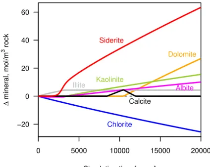
Figure 1 displays the outcome of the reference batch simulation. Anhydrite (not shown in the picture), is undersaturated at the beginning of the simulation and, being included as equilibrium phase in the model, is from the very first step of the simulation dissolved, staying substantially constant afterwards. Chlorite is dissolved and initially also albite. However, the latter inverts its trend and starts reprecipitating after around

25

(14)

GMDD

7, 6217–6261, 2014

M. De Lucia et al.

Title Page

Tables Figures

◭ ◮

Back Close

Full Screen / Esc

Discussion

P

a

per

|

Discus

sion

P

a

per

|

Discussion

P

a

per

|

Discussion

P

a

per

|

The most relevant feature of the model is the sequence of precipitating carbonate minerals. The first, starting from ca. 1500 simulation years, is the iron-bearing siderite, which is followed by a temporary appearance of calcite. Calcite starts redissolving as dolomite starts precipitating. Precipitation of siderite and dolomite continues until the end of simulation time. There is no appearance of magnesite in the model and a

negli-5

gible dissolution of hematite.

Prolonging the simulation to around 200 000 years sees the model approaching but not reaching an equilibrium state. At this point the precipitated volume of siderite reaches around 3000 cm3m−3of rock, or 0.3 % of the total rock volume. The precipita-tion of carbonates and illite, however, is partially compensated by dissoluprecipita-tion of

chlo-10

rite and anhydrite, and thus the calculated change in porosity after 200 000 years is

−0.00056 porosity units, which represents a relative change of around−0.11 % from

the initial value of 0.5. It can be safely considered negligible in terms of impact on the hydrodynamic properties of the medium.

3.2 Coupled simulations: spatial discretization and CO2injection 15

The simulation grid chosen for the coupled simulations in this study displays the typical complexity – and limitations – of reactive transport simulations in the domain of CO₂ storage, being coarse enough to allow for fully coupled reactive transport simulations in an affordable CPU time.

The spatial discretization of about 2.5 km×3.5 km near-field subset of the Stuttgart 20

formation of the Ketzin anticline comprises 2950 hexahedral elements arranged in one single layer with a 3-D structure following the topography of the target formation (Fig. 2). The thickness of the layer is around 75 m and thus comprises both main stratigraphic units of the Stuttgart Formation. Faults and discontinuities defined in the geological model have been geometrically smoothed in the one-layer model.

25

(15)

GMDD

7, 6217–6261, 2014

M. De Lucia et al.

Title Page

Tables Figures

◭ ◮

Back Close

Full Screen / Esc

Discussion

P

a

per

|

Discus

sion

P

a

per

|

Discussion

P

a

per

|

Discussion

P

a

per

|

build-up and is large enough that the injected CO₂does not arrive at the borders in the investigated time span.

Two distinct cases were investigated: an homogeneous medium with constant poros-ityϕ₌0.2 and permeability of 1×10−13m2and a spatially heterogeneous medium with

porosity ranging from 0.08 to 0.22 and permeability from 2.8×10−14to 3.0×10−12m2. 5

The heterogeneous distributions of porosity and permeability have been obtained by upscaling to the simulation grid respectively with arithmetic and geometric average the reservoir model described by Norden and Frykman (2013); Kempka et al. (2013a) and history-matched by Kempka and Kühn (2013). No further refinement of the upscaling was done, i.e., to obtain the same total pore volume in the simulation grids between

10

the homogeneous and heterogeneous cases, or more sophisticated permeability up-scaling.

The initial pressure for the models is set after equilibration runs assuming a hydro-static gradient. All simulations are isothermal at a temperature of 35◦

C. 67 000 t of CO₂ are injected at a constant rate in 5 years in the element highlighted in Fig. 2. This

rep-15

resents the amount of CO2 injected at the Ketzin site. After injection, the system is let

free to evolve until a total simulation time of 2200 years is reached.

It has to be stressed that the many adopted simplifications do not allow to consider the resulting model as an attempt to investigate the Ketzin site in a way coherent with the available monitoring data and previous modelling work. Again, the purpose of these

20

(16)

GMDD

7, 6217–6261, 2014

M. De Lucia et al.

Title Page

Tables Figures

◭ ◮

Back Close

Full Screen / Esc

Discussion

P

a

per

|

Discus

sion

P

a

per

|

Discussion

P

a

per

|

Discussion

P

a

per

|

4 Results

4.1 CO2migration in reactive and non-reactive simulations

For the purpose of this study it is important to evaluate the discrepancy between the reactive and fully coupled non-reactive simulations concerning the migration pattern of – and hence the reservoir volume exposed to – the injected CO2. The simplified

5

coupling is applied on the outcome of non-reactive simulations, and it must therefore be ensured that the bias with respect to the fully coupled simulations is quantitatively manageable. The reservoir volume exposed to the injected CO2, either gaseous or

dissolved, is therefore one of the crucial parameters in view of the application of the simplified coupling.

10

After injection, the CO2 would starts rapidly its migration mainly in upward direction

towards the anticline top, spreading and progressively dissolving in the formation brine along the way. Due to the coarseness of the simulation grid, the gaseous phase tends to progressively disappear, so that at the end of simulation time the majority of elements in which gas is still present display only a small residual gas saturation and almost

15

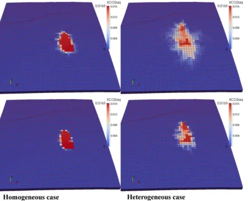
the whole injected CO2 is dissolved in the formation brine. The spatial distribution of

dissolved CO2 is displayed in Fig. 3, which collates snapshots after 2100 simulation

years for both the homogenous and heterogeneous cases. The significant differences in migration in the homogeneous and heterogeneous cases stem on one hand from the difference in total pore volume around the injection between the two simulations,

20

and on the other from the preferential flow paths which enhance the total spreading of the CO2(Lengler et al., 2010).

The non-reactive simulations show a quite enhanced spreading of the dissolved CO2

compared to the reactive case. However, this mainly consists of elements with small concentration located at the border of the CO2plume. Its central part, where the

high-25

(17)

GMDD

7, 6217–6261, 2014

M. De Lucia et al.

Title Page

Tables Figures

◭ ◮

Back Close

Full Screen / Esc

Discussion

P

a

per

|

Discus

sion

P

a

per

|

Discussion

P

a

per

|

Discussion

P

a

per

|

Figures 4 and 5 show the quantification of the exposed volumes respectively for the the homogeneous and the heterogeneous cases. In the diagrams the reservoir volume exposed to gaseous CO2(the black curves) is compared with the reservoir volume

ex-posed only to dissolved CO₂ in both fully coupled and non-reactive simulations (blue and red curves). It appears evident how soon after injection the reservoir elements

5

showing a gaseous phase reach a maximum and start decreasing immediately af-terwards. However, the discrepancy between reactive and non-reactive simulations is quite small in both cases: the presence of gas phase in an element is not significantly overestimated by the non reactive simulations.

Much more significant is the difference between the volumes exposed to dissolved

10

CO₂. Hereby two threshold values used to include the elements in the statistic are highlighted in blue and red, pointing out the large sensitivity of the outcomes on this choice. This is due to the fact that many elements are actually exposed only to low CO2

concentrations. Furthermore, a major discrepancy is found, both in the homogeneous and heterogeneous case, between the fully coupled and the non-reactive simulations:

15

the latter curves display a constant increase of exposed volume, whereas the reactive reach a maximum after around 500 years for the homogeneous case and around 1000 for the heterogeneous, afterwards substantially decreasing or hitting a plateau. This behavior actually means that in the non-reactive simulations the CO2plume continues

increasing its extent during the whole simulation time. Such discrepancy is actually

20

a measure of theoverestimationof the migration pattern caused by not accounting for chemical reactions.

However, the importance of the threshold, is not only spatial, but has also an im-pact on the definition of the considered exposure time. The larger the threshold, the later the arrival time of dissolved CO2is considered. In the simplified coupling the total

25

mineralization of the elements exposed only to dissolved CO₂ is limited on one hand to the actual maximum amount of CO2 reaching the element; but on the other it gets

also limited by the arrival time of CO2, which is retained as the starting point of the

(18)

GMDD

7, 6217–6261, 2014

M. De Lucia et al.

Title Page

Tables Figures

◭ ◮

Back Close

Full Screen / Esc

Discussion

P

a

per

|

Discus

sion

P

a

per

|

Discussion

P

a

per

|

Discussion

P

a

per

|

combination of its spatial and temporal effects which helps mitigating the overestima-tion of CO2migration returned by the non-reactive simulations.

In summary, the reservoir volume exposed to gaseous CO2is accurately predicted by

the non-reactive simulations and does not need a particular treatment. At the contrary, for the elements exposed only to dissolved CO2, the discrepancy between the

non-5

reactive and fully coupled reactive simulations is significant and imposes the choice of a threshold value for the CO₂ concentration considered geochemically active to miti-gate it.

4.2 Spatial self-similarity of reactions

The second major hypothesis is the self-similarity of chemical reactions in the fully

10

coupled simulations. In fact, the hypothesis underlying the simplified coupling is that the same reaction path is replicated in every element of the simulation grid, translated in time by the corresponding arrival time of CO2 and scaled according to the actual

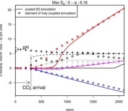
porosity and characteristic gas saturation of the element. Such replicated reaction path happens to be exactly the reference 0-D batch geochemical model depicted in Fig. 1.

15

The discrepancies among the elements of the coupled simulations can be imputed to the hydrodynamic transport of solute species, which is the only physical process responsible for “perturbing” the reactions, since by definition they all start from the same initial state in the whole domain.

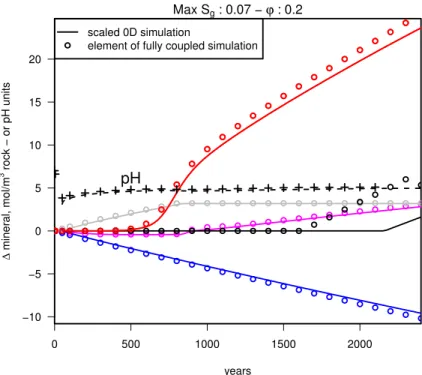
The comparison is visually represented in Figs. 6 and 7, which show two exemplary

20

elements taken respectively from the homogeneous and heterogeneous simulation. The first is an element exposed to gaseous CO2, while the second is exposed only to

dissolved CO2. The dotted lines represent the outcome of the fully coupled simulation

and the solid lines the output of the (scaled) 0-D model for one element of the simulation grid. The time axis of the scaled 0-D simulation have been translated to match the

25

actual arrival time of CO2in that element.

(19)

GMDD

7, 6217–6261, 2014

M. De Lucia et al.

Title Page

Tables Figures

◭ ◮

Back Close

Full Screen / Esc

Discussion

P

a

per

|

Discus

sion

P

a

per

|

Discussion

P

a

per

|

Discussion

P

a

per

|

in the majority of grid elements, which supports the hypothesis the simplified coupling is based on. Common discrepancies are represented by a slight delay in precipitation of some minerals (i.e. calcite in Fig. 6, the black line).

A numerical measure of the self-similarity is needed in order to control the initial hypothesis. This is achieved comparing the mineral changes in each element to the

5

0-D reference simulation. Noted with∆M_i the changes of a mineralM(in mass unit per m3rock) at the time stepsi ₌1,. . .,N from the fully coupled simulations and with∆M_i∗

the changes from the reference model (after translation of its time axis to match the arrival time of CO2 in the element), the similarity is defined as the average quadratic

relative error over the time samples:

10

Similarity=

v u u t1

N

N X

i=1

∆M_i−∆M∗ i

∆M∗ i

!2

(14)

From such definition follows that the similarity is a positive function, equal to zero if the compared reactions are exactly the same, and taking higher values for increasing discrepancy. Similarities can be computed for each mineral separately or for one of their possible linear combinations. In the following we will concentrate on the most

15

relevant linear combination for the purpose of this study, which is thetotal amount of precipitating carbonates.

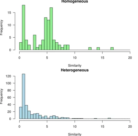
The results confirm that indeed the hypothesis of self-similarity holds: in Fig. 8 are shown the histograms of the calculated similarities for each element of the fully cou-pled simulations reached by CO2 in the homogeneous and heterogeneous case

re-20

spectively. For readability the histograms have been truncated to a value of 20 for the similarity function, which represents the 95th percentile in the homogeneous and the 99th percentile in the heterogeneous case. In both cases the vast majority of values are concentrated around 5 or less, with particularly small values – and thus high degree of similarity – for the heterogeneous simulations. Figures 6 and 7 display similarities

25

(20)

GMDD

7, 6217–6261, 2014

M. De Lucia et al.

Title Page

Tables Figures

◭ ◮

Back Close

Full Screen / Esc

Discussion

P

a

per

|

Discus

sion

P

a

per

|

Discussion

P

a

per

|

Discussion

P

a

per

|

discrepancy of total amount of mineralized CO₂ in the element is around 10 % at the end of the simulation time: in that particular case the delay in the mineralization of siderite and the temporary appearance of calcite explain such difference.

Figures 9 and 10 display the spatial distribution of the similariy function in the reser-voir, for the homogeneous and heterogenous cases. It appears that the best (lowest

5

values of the similarity function, in blue) similarities are located, in both cases, in the extern part of the CO₂ cloud, whereas the core part of the cloud show lower degree of similarity. On one side this is due to the longer exposure time and hence duration of reactive chemistry in such portion of reservoir, which amplificates and propagates the discrepancies; on the other side, this is an indirect measure of the influence of

hy-10

drodynamic transport: it is in the central portion of the cloud that the brine flow is the highest and thus most perturbs the chemistry.

In summary, for at least 95 % of the elements in which CO2 mineralization occurs,

the fully coupled simulations predict reactive chemistry which is qualitatively and quan-titatively nearly identical to the reference 0-D simulation. The second major hypothesis

15

for the application of the simplified coupling can be thus considered as verified.

4.3 Total mineralization

The next step is to evaluate the actual performance of the simplified coupling with respect to the outcome this method has been built for: the prediction of the total CO2

mineralization in the reservoir.

20

This result is shown in Fig. 11, highlighting the influence of the choice of the threshold on the result.

The diagram confirms that indeed the results of the simplified coupling (the dotted and the dashed lines) are quite on par with the outcome of the full coupling (the solid lines) for both the homogeneous and heterogeneous cases. It is also apparent that the

25

(21)

GMDD

7, 6217–6261, 2014

M. De Lucia et al.

Title Page

Tables Figures

◭ ◮

Back Close

Full Screen / Esc

Discussion

P

a

per

|

Discus

sion

P

a

per

|

Discussion

P

a

per

|

Discussion

P

a

per

|

nicely reproduced throughout the simulation time, with the exception of a slightly more significant deviation (in form of delay) in the first 500 simulation years for the homo-geneous simulation and around 1000 years in the heterohomo-geneous. After that, the sim-plified coupling approximates with excellent agreement the prediction of fully coupled simulations: under 3 % in terms of the total injected CO2.

5

Based on Fig. 11, a further consideration is possible, in particular from the observa-tion of the heterogeneous case (the blue curves). As result from the enhanced spread-ing of the injected CO2and the heterogeneity in porosity, contributing to the speed of

reactions, the mineralization is quite quick if compared with the homogeneous case, reaching a value of around 60 % of the injected CO₂ after 1700 years. Under these

10

conditions, a further prolongation of the simulation cannot be justified: the discrepancy in spreading and migration of CO2as estimated by the non-reactive simulations, which

are of course not accounting for the feedback of chemistry, will be obviously overesti-mated to an excessive degree, violating one of the hypotheses the simplified coupling is based on. Therefore, Fig. 11 is bounded on they axis: the outcome of the comparison

15

is not credible if the mineralization is too high.

The influence of the kinetics relative to the transport scenario was furthermore tested by replacing the chemical system considered until now with one with kinetic constants one order of magnitude smaller. The comparison procedure was repeated in an homo-geneous case, running the new 0-D batch geochemical model and the fully coupled

20

reactive transport, while the non-reactive simulations are the same as in the previous case. The considered simulation time for this case is 10 000 years. The outcome in terms of total mineralization is shown in Fig. 12.

Here one would expect that the slower kinetics would produce lower mineralization, and thus that the difference between reactive and non-reactive simulations would be

re-25

(22)

GMDD

7, 6217–6261, 2014

M. De Lucia et al.

Title Page

Tables Figures

◭ ◮

Back Close

Full Screen / Esc

Discussion

P

a

per

|

Discus

sion

P

a

per

|

Discussion

P

a

per

|

Discussion

P

a

per

|

explanation of this result is the decrease in self-similarity of reactions: in other words, for slower kinetics the relative importance of hydrodynamic transport of solutes be-comes more relevant, and thus one single geochemical model is less capable of rep-resenting the reactions in all elements of the spatial discretization. A faster kinetics would reinforce the hypothesis that only the presence of CO2in the element drives the

5

chemistry, reducing the relative importance of hydrodynamic transport. In this case it is more likely to experience more severe errors in the mass balance for the injected CO₂, which would also limit the applicability of simplified coupling approach.

In summary, the simplified coupling achieves an estimation of the total amount of mineralization which is in excellent agreement with the fully coupled simulations if an

10

optimal value for the threshold is employed.

5 Discussion and conclusion

5.1 The optimal choice for the threshold

A threshold value for the minimum dissolved CO2 concentration considered “active”

has been defined to filter out the overestimation of reservoir volume exposed to CO₂

15

(in both a spatial and a temporal sense) which comes from the non-reactive simula-tions. If too large, its choice can lead to severe underestimation, if too small, to severe overestimation of the total mineralization.

In a real application for the simplified coupling such optimal value is of course a priori unknown, since no fully coupled simulations are available. The strategy to determine

20

realistic values – or at least to define a realisticbandwidth– is always dependent on the investigated problem, and only guidelines can be outlined here.

A first consideration regards the proportion of elements exposed to dissolved CO2

in the simulations. In a typical storage system in saline aquifers, the reservoir volume exposed exclusively to dissolved CO₂can be much larger, in the time frame for which

25

(23)

GMDD

7, 6217–6261, 2014

M. De Lucia et al.

Title Page

Tables Figures

◭ ◮

Back Close

Full Screen / Esc

Discussion

P

a

per

|

Discus

sion

P

a

per

|

Discussion

P

a

per

|

Discussion

P

a

per

|

2013). However, the simulated concentration of dissolved CO₂ is often quite small, particularly at the front of the CO2plume.

Coarse spatial discretizations resulting in elements with very large volumes may induce an overestimation of the spatial extent of dissolved CO₂. In fact, most simulators allow the existance of gaseous CO2 in a separate, dense phase only if the dissolved

5

CO2excesses the saturation limit in the formation water in that element. Therefore, in

particular in presence of large volume elements, and particularly at the border of the CO2 plume, the presence (and hence propagation) of dissolved CO2 is favored with

respect to the gaseous phase, ending up in overestimating the total dissolved CO2.

Very small calculated concentrations of dissolved CO₂propagate to adjacent elements

10

to an extent which is not completely physical. Numerical dispersion may contribute to this effect. Notably, all these issues become more relevant for increasing coarseness of the simulation grid. Therefore, it can be expected that the fine hydrodynamic grids the simplified coupling is designed to be applied on should be far less sensitive to the threshold than the coarse model used in the present study for validation.

15

One-dimensional tests not showed in the present work support this hypothesis: through grid refinement not only the choice of threshold became less significant, but also the optimal threshold value was increased in the finer grids. Future work is how-ever needed to thoroughly assess this aspect. Another interesting option to explore in future work is the definition of a time-dependend threshold, and in particular increasing

20

along the progress of simulations.

A computational way to determine the optimal threshold is represented by the setup of 1-D or 2-D models mimicing the typical element dimension found in the full 3-D grid, the typical exposure time to CO2, and of course the same chemistry as in the original

model.

25

5.2 Applications and future work

(24)

GMDD

7, 6217–6261, 2014

M. De Lucia et al.

Title Page

Tables Figures

◭ ◮

Back Close

Full Screen / Esc

Discussion

P

a

per

|

Discus

sion

P

a

per

|

Discussion

P

a

per

|

Discussion

P

a

per

|

reservoir simulations, with no need to meet compromises such as the number of el-ements and the spatial heterogeneity described in the models.

This approach frees the reactive transport modelling from the limitations which ham-per many of its real life applications. It applies to hydrodynamic reservoir models, which are usualy well matched, without grid upscaling and therefore profiting of the best

pos-5

sible description of heterogeneity. This also includes boundary conditions and tran-sitory regimes (think about injection rate of CO₂ and its consequences on reservoir pressure), which are problematic to depict using oversimplified grids. The price for this ability – if all the hypotheses are met, which is usually the case in CO2 storage

sys-tems – is not a computational or numerical burden, but an approximation of the total

10

outcome of reactive chemistry, determined as bandwidth following the uncertainty of only one parameter: the concentration threshold.

Kempka et al. (2014) presents the application of the simplified coupling in the form described in the present work to a real-life scenario concerning the Ketzin pilot site. The simulation grid used for the hydrodynamic model amounts to 648 420 elements and the

15

simulation time reaches 16 000 years; it would have been impossible to achieve these results with the currently available fully coupled reactive transport simulators.

The storage in saline aquifer is actually an unfavorable case given its hydrodynamical complexity; much easier would be the case of CO2storage in depleted gas reservoirs,

where the water phase is present only in limited amount or residual saturations

(Audi-20

gane et al., 2009; De Lucia et al., 2012). In such cases the hypothesis of self-similarity of reactions will be met to an even better extent, since the solute transport in the for-mation brine will be quite reduced, if present at all.

The simplified approach is not limited to CO2 or gas storage, but can be employed

wherever its underlying assumptions are respected, and notably where the reactions

25

(25)

GMDD

7, 6217–6261, 2014

M. De Lucia et al.

Title Page

Tables Figures

◭ ◮

Back Close

Full Screen / Esc

Discussion

P

a

per

|

Discus

sion

P

a

per

|

Discussion

P

a

per

|

Discussion

P

a

per

|

A crucial application of the method is furthermore the ability to perform sensitivity and uncertainty analysis of the underlying components: both the hydrodynamic and the geochemical model. The advantage is of course represented by the separation of the processes, which can be therefore efficiently simulated on their own, and quickly “reassembled” in the post-processing approach, without the computational burden of

5

fully coupled simulations.

Finally, a combination of full coupling and simplified one-way coupling can be used for speeding up reactive transport simulations. Namely, in the framework of sequential coupling, in which at each time step first hydrodynamics is calculated on the simulation grid, and afterwards chemistry on each grid element, one could imagine to substitute

10

such expensive calculation of chemistry by scaling one single batch model as pro-posed in the simplified one-way approach. This would ensure consistency between CO2 available for transport and mineralized, eliminating the major uncertainty

con-nected to the application of the simplified approach in “post processing mode”. Also some other ideas presented in the present work could lead to improvements or further

15

computational speedups. In particular the check for self-similarity of reactions could be applied in heterogeneous settings in order to identify a reduced number of reaction paths that need to be actually included in the reactive transport simulations, much in a sense of the reduction of complexity of the chemical system discussed by De Lucia and Kühn (2013) or Hellevang et al. (2013).

20

6 Conclusions

The simplified one-way coupling introduced by Klein et al. (2013) has been validated by means of comparison with fully coupled reactive transport simulations in a typical CO2underground storage setting in a saline aquifer, exploring one homogeneous and

one heterogeneous case in terms of porosity and permeability. It was demonstrated

25

(26)

GMDD

7, 6217–6261, 2014

M. De Lucia et al.

Title Page

Tables Figures

◭ ◮

Back Close

Full Screen / Esc

Discussion

P

a

per

|

Discus

sion

P

a

per

|

Discussion

P

a

per

|

Discussion

P

a

per

|

0-D geochemical model can be used as proxy for the reactions occurring in all ele-ments of the simulation grid, and on the other side that the hydrodynamic transport of solutes plays a secondary role in comparison to the presence or not of the injected CO₂, which is the true driving force of the chemical reactions. The choice of athreshold valuefor dissolved CO2considered geochemically active governs the convergence of

5

the one-way coupling with the fully coupled simulations. This is particularly true for the given case study in which the migration of and exposure to dissolved CO₂represents the single most significant discrepancy between the non-reactive and the fully coupled simulations. For the considered case studies an optimal mass fraction concentration of around 0.0005 was found to ensure the best matching of the outcome of the fully

10

coupled simulations. Since in a real application this parameter is a priori unknown, the outcome of the simplified coupling has to be determined rather asbandwidth, for exam-ple by means of 1-D or 2-D simulations. However, given the advantage of performing coupled simulations on finely discretized grids with no simplifications and upscaling of heterogeneous features of the reservoirs, the uncertainty due to the simplified

cou-15

pling appears justified. Furthermore, removing the computational burden for reactive transport simulations makes the simplified approach particularly adapted to sensitiv-ity analyses, which are much needed given the uncertainty inherent to geochemical modelling.

Code availability 20

The analyses and methods outlined in this study are significant, in the opinion of the authors, rather from a methodological point of view than for their implementation, which is actually quite trivial and can be achieved using many different tools and programming environments. However, the R scripts (R Core Team, 2014) and the simulations needed to reproduce at least part of the presented results can be obtained directly contacting

25

(27)

GMDD

7, 6217–6261, 2014

M. De Lucia et al.

Title Page

Tables Figures

◭ ◮

Back Close

Full Screen / Esc

Discussion

P

a

per

|

Discus

sion

P

a

per

|

Discussion

P

a

per

|

Discussion

P

a

per

|

Acknowledgements. The authors gratefully acknowledge the funding for the Ketzin project received from the European Commission (6th and 7th Framework Program), two German ministries – the Federal Ministry of Economics and Technology and the Federal Ministry of Education and Research – and industry since 2004. The ongoing R&D activities are funded within the project COMPLETE by the Federal Ministry of Education and Research within the

5

GEOTECHNOLOGIEN program. Further funding is received by VGS, RWE, Vattenfall, Statoil, OMV and the Norwegian CLIMIT program.

The service charges for this open access publication have been covered by a Research Centre of the

10

Helmholtz Association.

References

Audigane, P., Gaus, I., Czernichowski-Lauriol, I., Pruess, K., and Xu, T.: Two-dimensional re-active transport modeling of CO₂injection in a saline aquifer at the Sleipner site, North Sea, Am. J. Sci., 307, 974–1008, doi:10.2475/07.2007.02, 2007. 6219

15

Audigane, P., Lions, J., Gaus, I., Robelin, C., Durst, P., der Meer, B. V., Geel, K., Oldenburg, C., and Xu, T.: Geochemical modeling of CO₂injection into a methane gas reservoir at the K12-B field, North Sea, AAPG Stud. Geol., 59, 499–519, 2009. 6240

Beyer, C., Li, D., De Lucia, M., Kühn, M., and Bauer, S.: Modelling CO₂-induced fluid–rock in-teractions in the Altensalzwedel gas reservoir. Part II: Coupled reactive transport simulation,

20

Environmental Earth Sciences, 67, 573–588, doi:10.1007/s12665-012-1684-1, 2012. 6219 De Lucia, M. and Kühn, M.: Coupling R and PHREEQC: efficient programming of geochemical

models, Energy Procedia, 40, 464–471, doi:10.1016/j.egypro.2013.08.053, 2013. 6241 De Lucia, M., Lagneau, V., de Fouquet, C., and Bruno, R.: The influence of

spa-tial variability on 2D reactive transport simulations, CR Geosci., 343, 406–416,

25

doi:10.1016/j.crte.2011.04.003, 2011. 6219

De Lucia, M., Bauer, S., Beyer, C., Kühn, M., Nowak, T., Pudlo, D., Reitenbach, V., and Stadler, S.: Modelling CO₂-induced fluid-rock interactions in the Altensalzwedel gas reser-voir. Part I: From experimental data to a reference geochemical model, Environmental Earth Sciences, 67, 563–572, doi:10.1007/s12665-012-1725-9, 2012. 6219, 6240