radar imaging observations with MAARSY
Svenja Sommer and Jorge L. Chau
Leibniz Institute of Atmospheric Physics at the University of Rostock, Kühlungsborn, Germany Correspondence to:Svenja Sommer ([email protected])
Received: 27 May 2016 – Revised: 21 November 2016 – Accepted: 22 November 2016 – Published: 19 December 2016
Abstract.A recent study has hypothesized that polar meso-spheric summer echoes (PMSEs) might consist mainly of lo-calized isotropic scattering. These results have been inferred from indirect measurements. Using radar imaging with the Middle Atmosphere Alomar Radar System (MAARSY), we observed horizontal structures that support our previous findings. We observe that small-scale irregularities, causing isotropic scattering, are organized in patches. We find that patches of PMSEs, as observed by the radar, are usually smaller than 1 km. These patches occur throughout the illu-minated volume, supporting that PMSEs are caused by lo-calized isotropic or inhomogeneous scattering. Furthermore, we show that imaging can be used to identify side lobe de-tections, which have a significant influence even for nar-row beam observations. Improved spectra estimations are ob-tained by selecting the desired volume to study parameters such as spectral width and to estimate the derived energy dissipation rates. In addition, a combined wide beam exper-iment and radar imaging is used to resolve the radial veloc-ity and spectral width at different volumes within the illumi-nated volume.
Keywords. Meteorology and atmospheric dynamics (turbu-lence; instruments and techniques) – radio science (remote sensing)
1 Introduction
Polar mesospheric summer echoes (PMSEs) are nowadays a well-understood phenomenon in the mesopause region, where turbulence plays a major role in the existence of these echoes in conjunction with charged ice particles and free electrons (Rapp and Lübken, 2004). These echoes are com-monly used as tracers for wind in polar regions in the
mid-dle atmosphere (e.g. Czechowsky et al., 1989; Stober et al., 2013) and are used to estimate the energy dissipation rate at mesospheric heights (Kelley et al., 1990).
and discuss the observations in relation to the Sommer et al. (2016a) findings.
The observation of PMSEs depends on the antenna beam pattern and, hence, the transmitting and receiving antenna. Large aperture radars such as Middle Atmosphere Alomar Radar System (MAARSY) have a strong side lobe suppres-sion of −17 dB (Latteck et al., 2012), but PMSEs can be stronger than that, and hence they can also be detected by side lobes (Chen et al., 2008). On the other hand, wind and turbulence estimation algorithms usually assume that the re-ceived signals come from the main beam (Hocking et al., 1986), which is not necessarily the case, especially if PMSEs are not equally distributed in the observation volume and/or they are stronger than the peak-to-side lobe level. Imaging techniques such as Capon (Palmer et al., 1998; Yu et al., 2001) or maximum entropy (Hysell and Chau, 2006) are ca-pable of resolving the scatter location within the beam vol-ume and are able to determine spectral parameters with their dependence on incident angle (Kudeki and Sürücü, 1991). This allows us to use the information either to identify what is really coming from the main beam or to lose the side lobe information to determine neutral dynamics.
In this paper, we present studies of PMSEs with coher-ent radar imaging (CRI) using Capon’s method. First, we show that PMSEs are composed of isotropic scattering that is horizontally inhomogeneously organized. Connected areas of isotropic scattering are here called patches. Theses patches are usually smaller than the beam volume. In the second part, we show how imaging can be used to identify side lobe detec-tions and apply a synthetic narrow beam for spectral analysis and energy dissipation rate determination.
2 Experimental setup and methods
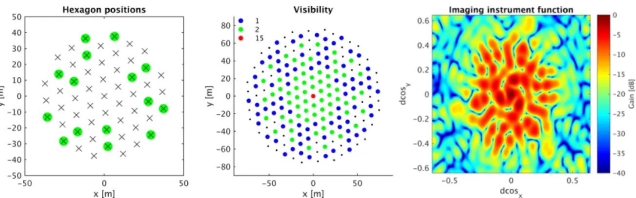
The Middle Atmosphere Alomar Radar System (MAARSY) is the only VHF (53.5 MHz) high-power large-aperture (866 kW) radar in northern polar regions capable of radar imaging. Its 433 Yagi antennas, each with its own transceiver module, are combined in groups of seven in a hexagonal structure. The whole array and 15 subarrays (or 16 subar-rays) can be sampled at once. To optimize the receiver con-figuration for radar imaging, a maximum of non-redundant baselines between all receivers is desirable. On 9 June 2015, MAARSY ran in the receiver configuration shown in Fig. 1, left side, with 145 unique baselines. The black crosses in-dicate possible receiver locations. However, MAARSY has a limited amount of 16 receiving channels. We chose 15 receiver locations, indicated by green circles, which are favourable for imaging, and one channel for the whole ar-ray. The visibility of the configuration is shown on the mid-dle panel of Fig. 1 to indicate the different baseline lengths and redundant baselines. The shortest baseline in this experi-ment was 10.6 m, the longest 73.3 m. The right panel of Fig. 1 shows the antenna beam pattern of the combined 15
subar-rays used for reception, i.e. the instrument function. For fur-ther MAARSY description, see Latteck et al. (2012).
Our radar imaging experiment was complemented with a narrow–wide beam configuration, meaning that two beam sizes of 3.6 and 12.6◦(half power full width (HPFW)) were transmitted almost simultaneously. The interpulse period of the experiment was 4 µs, and we expect that PMSEs change more slowly than that; hence we expect to observe the same PMSE with two different beam sizes. The beam direction was vertical with a range resolution of 150 m. The experi-ment had an interpulse period of 2 ms for each beam. Data were recorded after four coherent integrations, resulting in an effective time resolution of 8 ms. Continuous 32 s data blocks were recorded. Spectra estimation was done with two addi-tional coherent and four addiaddi-tional incoherent integrations. For further experiment details and parameters of the narrow– wide beam experiment, see Sommer et al. (2016a).
For this study, the data were analysed using Capon’s method (Capon, 1969; Palmer et al., 1998), as Capon’s method allows the direct access to the angular resolved spectral information and is adaptive to the data, unlike the Fourier method, and is able to suppress side-lobe contribu-tion. Capon’s method is fast and simple to implement com-pared to other methods such as maximum entropy and yields similar results in high signal-to-noise ratio (SNR) cases (Yu et al., 2000), which usually applies for PMSEs. The angular power distribution, called brightnessB, can be achieved by weighting each receiver signal with a linear filter to minimize side lobes adaptively and therefore possible interference. The resulting weighting vectorw(k) for a certain wavenumber
vector k=
θx θy θz, where θi is the direction cosine in x,y, andzdirection, respectively, can calculated as follows (Palmer et al., 1998):
wC= V
−1e
e†V−1e, (1)
wheree†represents the conjugate transpose of matrixe.
V=
V11 V12 . . . V1n V21 V22 . . . V2n
..
. ... ...
Vn1 Vn2 . . . Vnn
(2)
is the normalized cross-correlation matrix with the elements Vij=
hSiSj∗i
√
h|Si|2ih|Sj|2i
as the normalized cross correlation be-tween the signalsSi for receiversiandj (including also re-dundant baselines), and
e=eik·D1 eik·D2. . . eik·Dn, (3) whereDirepresents the centre of receiving arrayi.
The resulting brightness distribution is BC(k)=
1
Figure 1.Left: the receiving configuration of the imaging configuration in June 2015 is indicated by green circles. All possible receiving locations are indicated by black crosses. Middle: visibility function (as referred to by astrophysicists) for the imaging configuration. All possible baselines are indicated by black dots, and the colour code is the number of redundant baselines of the configuration used for imaging. Right: instrument function of the 15 hexagons indicated in the left panel. dcos is the direction cosine.
Capon’s method can be used not only for the angular power distribution but also to obtain radial velocities and spectral widths inside the beam volume, assuming quasi-stationarity during the observation period. For PMSEs, we obtain the spectrum for a certaink. Hence, we apply the weighting
vec-tor, obtained with the average of the time series, on the time series signalssof thenreceivers:
y(t )=w†
Cs(t ). (5)
The power spectral density for the parameter analysis is calculated by Fourier transforming each weighted time series for each pointing directionkand fitting a truncated Gaussian
function, yielding maps for the signal, Doppler velocity shift and spectral width.
The resulting radial velocities can be used to map the wind field. A simple approach such as a Doppler beam swinging (DBS) analysis could be applied, as well as more sophisti-cated approaches such as volume velocity processing, allow-ing for inhomogeneities in the wind field (Waldteufel and Corbin, 1979).
2.1 Results
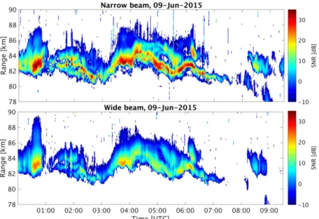
The signal-to-noise ratio (SNR) obtained from the narrow– wide beam experiment on 9 June 2015 is shown in Fig. 2. The top panel of Fig. 2 shows the SNR of the narrow beam with a beam width of 3.6◦HPFW. The lower panel of the
same figure shows the SNR of the wide beam (12.6◦HPFW)
experiment. The detection threshold for PMSEs was a SNR of −10 dB. During the observation time, PMSE occurrence was almost continuous at least in the narrow beam. Com-paring the results from both beams, the main features of the stronger PMSEs are observed in both beams, but the SNR of the wide beam is weaker than the SNR of the narrow beam. The most important reason is the geometry of the observa-tions: in the wide beam experiment, the power is spread over a larger solid angle, leading to less gain at zenith. If the beam
is wider, more energy will be transmitted to large off-zenith angles and scattered by PMSEs, but PMSEs appear in larger range gates at large off-zenith angles compared to a narrow beam. Decreasing the gain at zenith decreases therefore the SNR.
Due to the decreased SNR, some PMSEs cannot be de-tected (e.g. 07:30–08:30 UTC, 78–82 km) by the wide beam but can be seen in the narrow beam. On the other hand, sig-nal can be detected at larger ranges in the wide beam obser-vations than in the narrow beam obserobser-vations (e.g. 00:30– 01:00 UTC, 88–89.5 km).
The spectral parameters of the narrow beam experiment are shown in Fig. 3: (a) SNR, (b) radial Doppler velocity, (c) spectral width, (d) expected uncertainties for the Doppler velocity and (e) uncertainties for the spectral width. All the parameters are obtained from a truncated Gaussian fit like that used by Sheth et al. (2006). The red lines indicate two time intervals that are analysed later in detail with imaging. The Doppler velocity of the narrow beam varies mainly be-tween±15 m s−1 and are quite large compared to the ex-pected vertical wind component of only a few metres per second (Hoppe and Fritts, 1995) and indicate a horizontal wind contribution. Particularly large values (>15 m s−1) can be observed around 01:00 UTC above 88 km. The spectral width is sometimes enhanced during certain periods of time, e.g. 08:30–09:00 UTC, 83 to 85 km and 00:30–01:00 UTC, 85 km and above. The enhanced spectral width at the top of PMSEs, together with the increased corresponding radial velocity, is likely due to echoes coming from antenna side lobes, as we show below.
2.2 PMSE patch sizes
meth-Figure 2.RTI of the SNR from (top) narrow (3.6◦) and (bottom) wide (12.6◦) beam of the nested beam experiment on 9 June 2015.
Figure 3.Analysed parameters of the narrow beam (3.6◦).(a)SNR: the PMSE was strong during the observation time but got weaker in the last 2 h.(b)Doppler velocity: the radial velocity varies be-tween±15 m s−1.(c)The spectral width appears to be increased sometimes at the top of PMSE (00:00–01:00 UTC) or in the whole PMSE (08:00–09:00 UTC).(d)Doppler velocity error: error of the radial velocity estimation from the Gaussian fit.(e)Spectral width error: error of the width estimation from the Gaussian fit.
ods, like DBS or FCA, but these side lobe contributions could be estimated if the antenna beam pattern were known.
The remaining problem might be that the illuminated area is large and changes in PMSEs within the observed volume can occur. Therefore, using radar imaging, we analyse the
sizes of PMSE patches, i.e. areas with isotropic scattering, for different beam sizes and integration times. Such patches have been hypothesized by Sommer et al. (2016b).
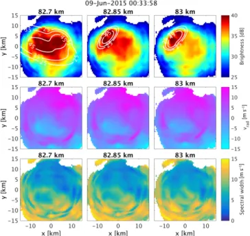
Figure 4 shows the obtained brightness (first row), radial velocity (second row) and spectral width (bottom row) for three adjunct altitudes after converting the image from angu-lar space and range into Cartesian coordinates and altitude with MAARSY at (0,0,0) for a 32 s wide beam data set. The limit for the maps was chosen to be a brightness of 25 dB to avoid presenting velocity and spectral width data with larger uncertainties. The white lines in the first row indicate fitted 2-D Gaussian ellipsoids. The point in time 00:33:58 UTC is marked by the first vertical red line in Fig. 3. The PM-SEs were strong at the time, and the observation volume was filled with PMSEs, which can be seen in the brightness dis-tribution. Although PMSEs occur in the whole beam volume, the strength varies. If PMSEs homogeneously filled the beam volume, the antenna beam pattern could be seen, which is not the case. In the lowest altitude, PMSEs fill almost homoge-neously the beam volume while at the highest altitude dis-played here, PMSEs are strongest in the upper left quadrant. In order to quantify the inhomogeneity, we fitted the peaks withN 2-D Gaussian ellipsoids (following Chau and Wood-man, 2001) of the form
f (x, y)= N
X
i=1
Aiexp −
x−x0i y−y0i
⊤
T⊤i 6i−1Ti
x−x0i y−y0i
!
+AN+1 (6)
with 6i=
2σxi 0 0 2σyi
Figure 4.Spectral parameters of PMSE after converting the image to Cartesian coordinates and altitude on 9 June 2015 00:33:58 UTC. The columns show three adjunct altitudes around the strongest PMSE altitude of 82.85 km. The brightness distributions are shown in the top row and are colour coded. The white lines indicate the fit-ted Gaussian ellipsoids. The middle row shows the radial velocities, indicating a horizontal wind, and the bottom row shows the imaged spectral width.
Ti =
cosθi sinθi
−sinθi cosθi
, (8)
whereAi is the amplitude,x0i andy0i are the centre coor-dinates,θi the anti-clockwise rotation angle, andσxiandσyi the width along major and minor axis of theith Gaussian el-lipsoid. The fitted ellipses are summed up and indicated by white lines. AN+1is the background brightness. The num-berNis determined by the number of peaks above a certain threshold.
The Doppler velocity is shown in the middle row of Fig. 4. The radial velocity becomes larger with increasing distance from the origin along the wind direction. This is reasonable with a horizontal wind component, given that the projected radial velocity depends on the off-zenith angle. The increase in radial velocity is not steady, indicating wind variability within the observed area. The belt of positive radial velocity that can be seen in all three images might be caused by spikes in the spectrum due to low SNR.
The spectral width is also not uniform (Fig. 4, bottom). Areas with increased brightness show a small spectral width while areas with increased spectral width occur mostly at larger distances from zenith, leading to an apparent larger spectral width.
Figure 5. Same as Fig. 4 but for 04:29:55 UTC and around
83.45 km.
A second example of PMSE images is shown in Fig. 5. It is similar to Fig. 4 but at 04:29:55 UTC. In contrast to Fig. 4, PMSEs are weaker and the beam volume is not completely filled. The radial velocities also indicate a horizontal wind field but show fewer variations than the wind field shown in Fig. 5. The spectral width maps do not show increased spectral width.
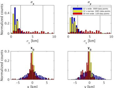
Figure 6.Histograms of the widths inxandydirection (top row) and centre locations (bottom row). For each figure, three histograms are shown. Yellow: 32 s narrow beam, blue: 32 s wide beam, red: 30 min wide beam
blue for 32 s integration period and in red for 30 min by aver-aging the spectra of the 32 s data set. The two black vertical lines indicate the 3 dB beam sizes at 85 km for the narrow (2.2 km) and wide beam (7.4 km), respectively. The bottom row shows the centre locations inxandydirection.
The patch sizes of the 32 s narrow and wide beams are rather similar with the peak of the size distribution under 2 km and therefore smaller than the narrow main beam inx as wellydirection. The wide beam patch distribution shows a shift to slightly larger values than the narrow beam patch distribution in both directions. This is probably due to the antenna beam pattern influence. The 30 min wide beam tribution does not show a distinct peak but a rather wide dis-tribution of patch sizes. This wider disdis-tribution might result from a non-homogeneous antenna beam pattern and imaging instrument function (see Fig. 2, right panel), as the Gaussian ellipsoid detection algorithm might detect only several dis-tinctive peaks. The second row shows the centre locations. All distributions are almost centred around the zenith but show different widths. The 32 s narrow beam centre distri-butions in x andy direction have the smallest width as the centre location is limited by the antenna beam pattern. The 32 s wide beam centre distributions have the broadest width, as patches of PMSEs can occur in a larger beam volume, and hence the spread is larger than in the narrow beam centre distribution. On the other hand, the 30 min wide beam cen-tre distributions are narrower than the 32 s distribution. With longer integration time, the antenna beam pattern should be-come more dominant and reduces the patchiness of PMSEs, resulting in a more centred distribution for the narrow beam.
2.3 Enhanced spectral width
The distinction between main beam and side lobe detection is crucial. Even with a strong side lobe attenuation of−17 dB of the first side lobe for its standard narrow beam, MAARSY is able to receive significant contributions of signals from the side lobes when strong PMSEs occur. Therefore, we show a way to identify the side lobe signals and improve the esti-mates of radial velocity and spectral width.
To identify main beam and side lobe detections, we apply radar imaging as described above, resulting in a spectrum for each virtual beam pointing directionk. Each spectrum was
analysed regarding Doppler velocity and spectral width. In order to avoid large angle contributions, we use imag-ing and compare the results to the standard narrow beam, for which we assume that all echoes come from the main beam. We averaged the spectra, obtained from imaging, only for a certain area, namely between−1.8 and 1.8◦, hereafter called
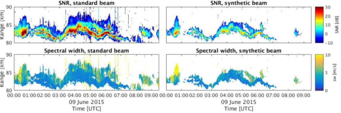
synthetic narrow beam, and determined the spectral width from the average of the spectra. The area corresponds to the HPFW main beam of MAARSY. Figure 7 shows range time intensity plots (RTIs) of the SNR and spectral width for the standard narrow beam (left column) and the synthetic narrow beam (right column). It can be seen that the spectral width of the standard narrow beam shows sometimes an increase at the upper edge of PMSEs. These features vanishes when the spectrum is only obtained from the synthesized narrow beam. This can be clearly seen around 06:20 UTC around 85 km. However, there are periods with increased spectral width in the synthetic narrow beam, possibly related to increased tur-bulence, e.g. around 08:00 UTC.
We used the approach of Hocking (1985) to estimate the turbulence strength in a simple approach by neglecting shear and wave broadening (Murphy et al., 1994; Nastrom and Eaton, 1997). We estimated the horizontal wind velocity us-ing the derived radial velocity maps presented above usus-ing a DBS approach. The resulting wind magnitude of the hor-izontal wind is presented in Fig. 8, top. Throughout the ob-servation period, increased periods of wind can be detected, leading to an increased spectral width due to beam broaden-ing. Following Hocking (1985), the turbulence strengthǫcan be derived from the HPFW of the spectrum by
fturb2 =fobs2 −fbb2, (9)
wherefturb is the increase in spectral width due to turbu-lence,fobsis the measured HPFW of the spectrum andfbb=
2
Figure 7.Comparison of spectral parameters obtained from the standard narrow beam, including side lobes (left column), and the synthetic narrow beam (right column). The synthetic narrow beam was obtained by gaining spectra for each virtual beam pointing directionkand average the resulting spectra only between−1.8 and 1.8◦. Comparing the SNR (first row), the echoes from the upper edges of PMSEs are removed in the main beam while the lower edges are in the same range. Signals with large spectral width (second row) due to side lobe detections are removed from the beam and increased spectral width to turbulence remains.
Figure 8.Top: magnitude of the horizontal wind velocity derived by DBS from Doppler velocity maps. Middle: derived energy dissipation rate for the standard narrow beam. Bottom: derived turbulent energy dissipation rate for a synthetic narrow beam.
which, however, is zero outside the MAARSY main beam (i.e.>1.8◦).
The mean square fluctuation velocityv2rmsis given by
v2rms=λ 2
4 fturb2
2 ln 2 (10)
yielding forǫ:
ǫ=CN vrms2 , (11)
whereC is a numerical constant andN the Brunt–Väisäla-frequency. Here, we use typical values for the polar meso-sphere, i.e.C=0.47 andN=0.0134 rad s−1(Gibson-Wilde et al., 2000). The results forǫare presented in Fig. 8, mid-dle, for the standard narrow beam, including side lobe con-tributions, and in the bottom panel for the synthetic narrow
Figure 9.Histogram for the energy dissipation rate forǫderived by the narrow beam and the synthetic narrow beam. Top left: 2-D correlation inǫbetween the standard narrow beam and the synthetic narrow beam. The red line indicatesx=y. A deviation can be seen especially for smallǫ. The cumulative histograms alongxandydirection are shown in the top right and lower panels, respectively. The red line shows the cumulative histogram for the standard narrow beam and the blue line for the synthetic narrow beam.
beam. For better comparison, the other histogram is shown with a dashed line. For low energy dissipation rates, com-paring the standard narrow beam and the synthetic narrow beam, a shift towards lower energy dissipations rates can be seen here also. That means that correcting for side lobe con-tribution affects mainly low-turbulence cases.
2.3.1 Discussion
The horizontal variation on larger scales have been inves-tigated by multi-beam experiments (Latteck et al., 2012; Stober et al., 2013). They showed that PMSEs can vary within observation volumes of 80 km diameter by 40 dB in SNR. Multi-beam experiments take time and the resolution is limited by the beam size. Röttger et al. (1990) concluded from spectral observations that PMSEs at 224 MHz must be smaller than their observation volume, i.e. 1 km in vertical and horizontal extent. To investigate the horizontal structure of PMSEs further and quantify the localized scattering, we applied Capon’s method of imaging. As shown in the re-sults section above, PMSEs vary in altitude, horizontal lo-cation and extent. PMSEs are composed of isotropic scatter-ing organized in horizontally contiguous areas. Sometimes, the beam volume is filled completely with isotropic scatter-ing, but the angular power distribution is not homogeneous
(Fig. 4). In other cases, PMSEs appear in patches of isotropic scattering that are asymmetric and can be smaller than 1 km. Even with the narrow beam experiment with a beam width of 3.6◦, the brightness distribution within the observation vol-ume is not homogeneous. It can be seen in Fig. 6 that the narrow and wide beam patches for 32 s integration time are of the same order of magnitude, although one would expect that the antenna beam pattern has a major influence. This might be due to the receiving antenna pattern, which is limited by the receiver configuration (compare to Fig. 1). Furthermore, the centre location of especially the wide beam patches is slightly shifted towards negativey0. This is probably due to a small phase calibration offset but the main features of PM-SEs are preserved.
resolution of the radars used in these studies is lower than the resolution presented in this paper and smaller structures might not have been resolved. Furthermore, we showed that PMSE backscatter can be received from the whole beam vol-ume, which makes it unlikely to be aspect-sensitive scatter-ing. Still, the structure of the isotropic scattering can be in-fluenced by gravity waves as suggested by Chen et al. (2008) for the reflection type of scattering.
The inhomogeneous structure is due to the nature of PM-SEs. As Rapp and Lübken (2004) pointed out, three major components must be present for PMSEs to exist: negatively charged ice particles, free electrons and turbulence. Baum-garten and Fritts (2014, Fig. 2) showed in NLC observations that ice particles in mesospheric altitudes also show wave structures with short wavelengths (<20 km) when ice parti-cles are moved to different altitudes. Hence, it is not surpris-ing that PMSEs, bound to the existence of these ice particles, display also wave structures on the small scale.
In addition to the patchy structure, we observe enhanced brightness within the observation volume, when PMSEs fill the complete beam volume. This might be caused by local-ized enhanced turbulence or electron density but needs fur-ther investigation.
The non-homogeneous PMSE distribution in space has ef-fects on measurement techniques for wind and/or turbulence estimations such as DBS or FCA. FCA is, as an in-beam es-timation method, especially influenced by small-scale wave activity, as the ground diffraction pattern is used to determine atmospheric parameters. Usually, the derivation required a statistically homogeneous scatter distribution with a verti-cal anisotropy (Doviak et al., 1996) or additional anisotropy inx andy direction (Holloway et al., 1997). In addition to the anisotropy of the scattering mechanism, the scatter itself might not be statistically homogeneously distributed in the observation volume, which can lead to an underestimation of the horizontal wind velocity (Holdsworth, 1995). This might be due to localized enhancements, patches or waves. Usually, the sampling time used for FCA is about 30 s as used in the results presented here. We showed that, on these timescales, the distribution of PMSEs in the beam volume is not homo-geneous. The non-homogeneity leads to an increased cor-relation compared to a statistically homogeneous scattering process and was previously interpreted as aspect sensitivity. Sommer et al. (2016b) compared aspect sensitivity values
ob-The assumption is that the scattering mechanism is isotropic and also homogeneous. We have shown above that on short timescales the assumption of a homogeneous scattering pro-cess is not nepro-cessarily given, resulting in a smaller volume reflectivity factor. This can be solved by calculating a beam-filling factor for the volume reflectivity or, following the ap-proach of Sommer et al. (2016b), by using longer integration periods. Latteck and Bremer (2013) used integration times of 5 min, which smoothes the localized signals and is already 10 times longer than the data sets presented here, while even longer integration periods would be more favourable.
In the second part of the discussion, we discuss radar imaging to remove side lobe detections. Mesosphere– stratosphere–troposphere (MST) radars like MAARSY are used to study atmospheric parameters such as radial veloc-ities for wind estimations and spectral width for turbulence estimations. Sensitive radar systems have a good side lobe suppression (e.g. MAARSY−17 dB one way; Latteck et al., 2012). The suppression of MAARSY is better than older sys-tems like ALWIN (Alomar wind radar) (−13 dB one way, Latteck et al., 1999), but MAARSY still receives significant backscatter from the side lobes. If these side lobe detections are not separated from the main beam detections, the results are compromised. In this paper, we showed that, with the help of imaging, side lobe detections of PMSEs could be re-duced significantly. The cleaned spectrum, only for the main beam, can now be analysed regarding the spectral parame-ters. As shown above, the side lobe detections have a major influence on the spectral width and therefore on turbulence estimations. On the other hand, we can use the information from the side lobes with imaging to resolve the spectral width and Doppler velocity in space as shown in Sect. 2.2.
(2004) expected ǫ=5 mW kg−1, while Gibson-Wilde et al. (2000) simulated values up to ǫ=150 mW kg−1 using a direct numerical simulation. Li et al. (2010) found en-ergy dissipation rates using the European Incoherent Scat-ter Svalbard Radar at 500 MHz (Bragg wavelength 30 cm) of ǫ=5–200 mW kg−1. Our observations agree also well with in situ measurements. Sounding rocket flights con-ducted by Lübken et al. (2002) measured values between ǫ=0 mW kg−1andǫ∼2400 mW kg−1 in the mesosphere. The mean value where PMSEs and turbulence coincided in the flights wasǫ=390 mW kg−1with a rather large standard deviation of 190 mW kg−1.
We also found strong turbulent events within PMSEs, even after removing side lobe contribution and beam broadening. Strong turbulent events showed ǫ >500 mW kg−1, which exceeds the expected theoretical values but still agrees with the sounding rocket measurements of Lübken et al. (2002). Furthermore, we showed that the corrections made in this pa-per affect the majority of low-turbulence cases. For high tur-bulence values, the synthetic narrow beam and the standard narrow beam values correlate well.
In this calculation, we neglected shear broadening as the range resolution is high and the shear contribution probably small compared to the other effects (Strelnikova and Rapp, 2011). We neglected also wave broadening, which would allow for high-frequency gravity waves. Still, the observed spectral width should exceed the contribution of shear and wave broadening and is therefore an indicator of strong tur-bulence. The analysis presented here should be expanded in future to include shear and beam broadening effects, which might have a significant contribution in weak turbulence measurements.
3 Conclusions
In this paper, we showed that PMSEs appear sometimes in horizontally contiguous areas, or patches, smaller than even 1 km, usually in patches with a few kilometres in diameter, and sporadically comparable in size to the observed volume (∼20 km) using radar imaging. Large patches of PMSEs can be observed on some occasions, but these patches are not ho-mogeneous. These inhomogeneities can be explained by an isotropic scattering mechanism that is probably influenced by the background dynamics, creating the patchiness. Long integration periods could be used to smooth out the patchy nature of PMSEs for experiments that do not require a high temporal resolution. The patchy structure of PMSEs might be misinterpreted as aspect sensitivity, which should be con-sidered in future investigations of PMSEs.
Furthermore, we showed that radar imaging can be used to identify side lobe contributions in spectral width that occur even in modern radar systems like MAARSY. The method presented here can be used to improve turbulence measure-ments with MST radars. We found that the correction is
sig-nificant most of the time in the analysed data. Events charac-terized by high spectral width show similar turbulence values before and after the beam broadening corrections.
4 Data availability
The raw data are not openly available since they are being used for other research topics. However, those interested can contact Jorge Chau ([email protected]) to get limited ac-cess to the data.
Acknowledgements. The authors thank the MAARSY team, es-pecially Ralph Latteck for his support during the imaging cam-paign, Toralf Renkwitz for providing the wide beam phases and also Bjørn Gustavsson from University of Tromsø for his help choos-ing the imagchoos-ing configuration. We also thank Gunter Stober for providing the spectral fit algorithm used in the imaging analysis. Svenja Sommer was supported by ILWAO.
The topical editor, C. Jacobi, thanks two anonymous referees for their help in evaluating this paper.
References
Baumgarten, G. and Fritts, D. C.: Quantifying Kelvin-Helmholtz instability dynamics observed in noctilucent clouds: 1. Meth-ods and observations, J. Geophys. Res., 119, 9324–9337, doi:10.1002/2014JD021832, 2014.
Briggs, B. H.: On the analysis of moving patterns in geophysics– I. Correlation analysis, J. Atmos. Terr. Phys., 30, 1777–1788, 1968. Capon, J.: High-Resolution Frequency-Wavenumber Spectrum
Analysis, IEEE Proc., 57, 1408–1418, 1969.
Chau, J. L. and Woodman, R. F.: Three-dimensional coherent radar imaging at Jicamarca: comparison of different inversion tech-niques, J. Atmos. Sol.-Terr. Phy., 63, 253–261, 2001.
Chen, J.-S., Hoffmann, P., Zecha, M., and Hsieh, C.-H.: Coherent radar imaging of mesosphere summer echoes: Influence of radar beam pattern and tilted structures on atmospheric echo center, Radio Sci., 43, RS1002, doi:10.1029/2006RS003593, 2008. Chilson, P. B., Yu, T.-Y., Palmer, R. D., and Kirkwood, S.: Aspect
sensitivity measurements of polar mesosphere summer echoes using coherent radar imaging, Ann. Geophys., 20, 213–223, doi:10.5194/angeo-20-213-2002, 2002.
Czechowsky, P., Reid, I. M., Rüster, R., and Schmidt, G.: VHF Radar Echoes Observed in the Siummer and Winter Polar Meso-sphere Over Andøya, Norway, J. Geophys. Res., 94, 5199–5217, 1989.
Doviak, R. J., Lataitis, R. J., and Holloway, C. L.: Cross correlations and cross spectra for spaced antenna wind profilers: 1. Theoreti-cal analysis, Radio Sci., 31, 157–180, 1996.
Gibson-Wilde, D., Werne, J., Fritts, D., and Hill, R.: Di-rect numerical simulation of VHF radar measurements of turbulence in the mesosphere, Radio Sci., 35, 783–798, doi:10.1029/1999RS002269, 2000.
1. Motion field characteristics and measurement biases, J. Geo-phys. Res., 100, 16813–16825, 1995.
Hysell, D. L. and Chau, J. L.: Optimal aperture synthesis radar imaging, Radio Sci., 41, 1–12, doi:10.1029/2005RS003383, 2006.
Kelley, M., Ulwick, J., Röttger, J., Inhester, B., Hall, T., and Blix, T.: Intense turbulence in the polar mesosphere: rocket and radar measurements, J. Atmos. Terr. Phys., 52, 875–891, doi:10.1016/0021-9169(90)90022-F, 1990.
Kudeki, E. and Sürücü, F.: Radar interferometric imaging of field-aligned plasma irregularities in the equatorial electrojet, Geo-phys. Res. Lett, 18, 41–44, doi:10.1029/90GL02603, 1991. Latteck, R. and Bremer, J.: Long-term changes of polar mesosphere
summer echoes at 69◦N, J. Geophys. Res., 118, 10441–10448, doi:10.1002/jgrd.50787, 2013.
Latteck, R., Singer, W., and Bardey, H.: The ALWIN MST Radar: Technical Design and Performance, European Rocket and Bal-loon Programs and Related Research, Proceedings of the 14th ESA Symposium held 31 May–3 June, 1999, Potsdam, edited by: Schürmann, B., European Space Agency, ESA-SP, 437, 179– 184, 1999.
Latteck, R., Singer, W., Rapp, M., Vandepeer, B., Renkwitz, T., Zecha, M., and Stober, G.: MAARSY: The new MST radar on Andøya-System description and first results, Radio Sci., 47, RS1006, doi:10.1029/2011RS004775, 2012.
Li, Q., Rapp, M., Röttger, J., Latteck, R., Zecha, M., Strelnikova, I., Baumgarten, G., Hervig, M., Hall, C., and Tsutsumi, M.: Mi-crophysical parameters of mesospheric ice clouds derived from calibrated observations of polar mesosphere summer echoes at Bragg wavelengths of 2.8 m and 30 cm, J. Geophys. Res., 115, D00I13, doi:10.1029/2009JD012271, 2010.
Lübken, F.-J., Rapp, M., and Hoffmann, P.: Neutral air tur-bulence and temperatures in the vicinity of polar meso-sphere summer echoes, J. Geophys. Res., 107, 4273, doi:10.1029/2001JD000915, 2002.
Murphy, D., Hocking, W., and Fritts, D.: An assessment of the effect of gravity waves on the width of radar Doppler spectra, J. At-mos. Terr. Phys., 56, 17–29, doi:10.1016/0021-9169(94)90172-4, 1994.
Swartz, W. E.: Polar mesosphere summer echoes observed with the EISCAT 933-MHz radar and the CUPRI 46.9-MHz radar, their similarity to 224-MHz radar echoes, and their relation to turbulence and electron density profiles, Radio Sci., 25, 671–687, doi:10.1029/RS025i004p00671, 1990.
Sheth, R., Kudeki, E., Lehmacher, G., Sarango, M., Woodman, R., Chau, J., Guo, L., and Reyes, P.: A high-resolution study of mesospheric fine structure with the Jicamarca MST radar, Ann. Geophys., 24, 1281–1293, doi:10.5194/angeo-24-1281-2006, 2006.
Smirnova, M., Belova, E., and Kirkwood, S.: Polar mesosphere summer echo strength in relation to solar variability and geomag-netic activity during 1997–2009, Ann. Geophys., 29, 563–572, doi:10.5194/angeo-29-563-2011, 2011.
Sommer, S., Chau, J. L., and Schult, C.: On high time-range res-olution observations of PMSE: statistical characteristics, J. Geo-phys. Res., 121, 6713–6722, doi:10.1002/2015JD024531, 2016a. Sommer, S., Stober, G., and Chau, J. L.: On the angu-lar dependence and scattering model of Poangu-lar Mesospheric Summer Echoes at VHF, J. Geophys. Res., 121, 278–288, doi:10.1002/2015JD023518, 2016b.
Stober, G., Sommer, S., Rapp, M., and Latteck, R.: Investigation of gravity waves using horizontally resolved radial velocity mea-surements, Atmos. Meas. Tech., 6, 2893–2905, doi:10.5194/amt-6-2893-2013, 2013.
Strelnikova, I. and Rapp, M.: Majority of PMSE spectral width at UHF and VHF are compatible with a single scattering mecha-nism, J. Atmos. Sol.-Terr. Phy., 73, 2142–2152, 2011.
Waldteufel, P. and Corbin, H.: On the analysis of single Doppler data, J. Appl. Meteorol., 18, 53–542, 1979.
Yu, T. Y., Palmer, R. D., and Hysell, D. L.: A simulation study of coherent radar imaging, Radio Sci., 35, 1129–1141, 2000. Yu, T.-Y., Palmer, R. D., and Chilson, P. B.: An investigation of
scattering mechanisms and dynamics on PMSE using coherent radar imaging, J. Atmos. Sol.-Terr. Phy., 63, 1797–1810, 2001. Zecha, M., Röttger, J., Singer, W., Hoffmann, P., and Keuer, D.: