Determining water sources in the boundary layer from tall tower profiles of water vapor and surface water isotope ratios after a snowstorm in Colorado

(1)

ACPD

12, 16327–16375, 2012

Determining water sources in the boundary layer

D. Noone et al.

Title Page

Abstract Introduction

Conclusions References

Tables Figures

◭ ◮

Back Close

Full Screen / Esc

Printer-friendly Version Interactive Discussion

Discussion

P

a

per

|

Dis

cussion

P

a

per

|

Discussion

P

a

per

|

Discussio

n

P

a

per

|

Atmos. Chem. Phys. Discuss., 12, 16327–16375, 2012 www.atmos-chem-phys-discuss.net/12/16327/2012/ doi:10.5194/acpd-12-16327-2012

Atmospheric Chemistry and Physics Discussions

This discussion paper is/has been under review for the journal Atmospheric Chemistry and Physics (ACP). Please refer to the corresponding final paper in ACP if available.

Determining water sources in the

boundary layer from tall tower profiles of

water vapor and surface water isotope

ratios after a snowstorm in Colorado

D. Noone1,2, C. Risi1,2,*, A. Bailey1,2, M. Berkelhammer1,2, D. P. Brown1,2, N. Buenning1,2,**, S. Gregory1,2,***, J. Nusbaumer1,2, D. Schneider1,2,****, J. Sykes1,2, B. Vanderwende1, J. Wong1,2, Y. Meillier2, and D. Wolfe2,3

1

Department of Atmospheric and Oceanic Sciences, University of Colorado, Boulder, CO, USA 2

Cooperative Institute for Research in Environmental Sciences, University of Colorado, Boulder, CO, USA

3

Physical Sciences Division, Earth System Research Laboratory, National Oceanic and Atmospheric Administration, Boulder, CO, USA

*

now at: Laboratoire de M ´et ´eorologie Dynamique, Paris, France **

now at: Department of Earth Sciences, University of Southern California, Los Angeles, CA, USA

***

now at: Precision Wind Inc., Boulder, CO, USA ****

(2)

ACPD

12, 16327–16375, 2012

D. Noone et al.

Title Page

Tables Figures

◭ ◮

Back Close

Full Screen / Esc

Discussion

P

a

per

|

Dis

cussion

P

a

per

|

Discussion

P

a

per

|

Discussio

n

P

a

per

|

Received: 24 April 2012 – Accepted: 18 May 2012 – Published: 4 July 2012

Correspondence to: D. Noone ([email protected])

(3)

ACPD

12, 16327–16375, 2012

D. Noone et al.

Title Page

Tables Figures

◭ ◮

Back Close

Full Screen / Esc

Discussion

P

a

per

|

Dis

cussion

P

a

per

|

Discussion

P

a

per

|

Discussio

n

P

a

per

|

Abstract

The D / H isotope ratio is used to attribute boundary layer humidity changes to the set of contributing fluxes for a case following a snowstorm in which a snow pack of about 10 cm vanished. Profiles of H₂O and CO₂mixing ratio, D / H isotope ratio, and several thermodynamic properties were measured from the surface to 300 m every 15 min dur-5

ing four winter days near Boulder, Colorado. Coeval analysis of the D / H ratios and CO₂concentrations find these two variables to be complementary with the former be-ing sensitive to daytime surface fluxes and the latter particularly indicative of nocturnal surface sources. Together they capture evidence for strong vertical mixing during the day, weaker mixing by turbulent bursts and low level jets within the nocturnal stable 10

boundary layer during the night, and frost formation in the morning. The profiles are generally not well described with a gradient mixing line analysis because D / H ratios of the end members (i.e., surface fluxes and the free troposphere) evolve throughout the day which leads to large uncertainties in the estimate of the D / H ratio of surface water flux. A mass balance model is constructed for the snow pack, and constrained with 15

observations to provide an optimal estimate of the partitioning of the surface water flux into contributions from sublimation, evaporation of melt water in the snow and evapo-ration from ponds. Results show that while vapor measurements are important in con-straining surface fluxes, measurements of the source reservoirs (soil water, snow pack and standing liquid) offer stronger constraint on the surface water balance. Measure-20

ments of surface water are therefore essential in developing observational programs that seek to use isotopic data for flux attribution.

1 Introduction

The representation of the land surface energy and water budget is a significant source of dispersion between climate model projections of future changes in temperature and 25

(4)

ACPD

12, 16327–16375, 2012

D. Noone et al.

Title Page

Tables Figures

◭ ◮

Back Close

Full Screen / Esc

Discussion

P

a

per

|

Dis

cussion

P

a

per

|

Discussion

P

a

per

|

Discussio

n

P

a

per

|

et al., 2000; Boe and Terray, 2008) or land use changes (Pitman et al., 2009). Land-atmosphere interactions also play a key role in the meteorological and hydrological variability at different times scales from weeks to decades (Avissar and Werth, 2005; Milly et al., 2005; Bosilovich and Chern, 2006; Guo et al., 2006; Koster et al., 2006). Inadequate representation of surface fluxes and their dependence on surface condi-5

tions are among the key sources of uncertainties in quantifying regional hydroclimate (Koster and Milly, 1997; Gedney et al., 2000; Boone et al., 2004). A particularly vexing subset of this issue arises in regions covered by snow, where the representation of processes in the snow pack is largely unconstrained (Slater et al., 2001; Boone et al., 2004; Rutter et al., 2009). Additional surface flux uncertainties arise from imperfect de-10

piction of boundary layer processes, notably under stable conditions (Holtslag, 2006). Reducing these uncertainties requires better understanding of the movement of water between the landscape and the atmosphere.

Because the stable hydrogen and oxygen isotope ratio of water vapor, liquid and ice reflects the balance of processes influencing regional hydrology, measurements of 15

the oxygen and hydrogen isotope ratios of water can provide constraints for water bal-ance studies and expose model shortcomings (Jouzel and Merlivat, 1984; Henderson-Sellers et al., 2004; Henderson-Henderson-Sellers, 2006; Sturm et al., 2010). The utility of iso-tope ratio information stems from the fractionation that accompanies phase changes in which the heavier isotopologues preferentially remain in liquid or solid form during 20

evaporation and condensation (Bigeleisen, 1961; Dansgaard, 1964). At the continental scale, the distributions of the isotopic composition of precipitation have been used to partition continental recycling into evaporation from standing water and transpiration (Salati et al., 1979; Gat and Matsui, 1991). At the local scale, isotopic measurements of water vapor and soil water have been used to partition evapotranspiration into tran-25

(5)

ACPD

12, 16327–16375, 2012

D. Noone et al.

Title Page

Tables Figures

◭ ◮

Back Close

Full Screen / Esc

Discussion

P

a

per

|

Dis

cussion

P

a

per

|

Discussion

P

a

per

|

Discussio

n

P

a

per

|

1999; Ehhalt et al., 2005; Angert et al., 2008; Noone et al., 2011). However, studies to date have been limited by the availability of measurements of water vapor isotopic ratios.

A common approach in water source partitioning is to estimate the isotopic com-position of the total surface flux. This is typically estimated using a “Keeling plot” ap-5

proach (Keeling, 1958; Pataki et al., 2003) which is based on a simple two-member mixing model. This technique has been applied to both temporal series (e.g., Moreira et al., 1997; Noone et al., 2011; Noone, 2012) and vertical profiles (Yepez et al., 2003; Williams et al., 2004). However there is some evidence from CO2 and

13

C measure-ments from tall towers that both have limitations due to advection that invalidates the 10

assumptions underlying the method (Griffis et al., 2007). With the advent of field de-ployable water vapor isotopic instruments, many of the previous technical limitations in obtaining water vapor isotopic data have been overcome and high frequency mea-surements can now be performed (e.g., Lee et al., 2007; Gupta et al., 2009; Wang et al., 2010). Such measurements allow reexamination of the mixing line method and the 15

question of how to attribute fluxes to multiple contributing components.

In this paper, we test the use of isotopic information to decompose surface latent heat flux into different physical components. The flux attribution calculation employs mass balance to partition the flux associated with loss of the snow pack into sublimation and evaporation from melt ponds and employs a maximum likelihood estimation approach 20

to provide an optimal estimate in the under-constrained problem. The technological improvement in observational capacity is exploited to measure vertical profiles of water vapor isotopic composition within the boundary layer from the surface to 300 m near Boulder, Colorado at a vertical resolution of a few tens of meters every 15 min. The study focuses on results from a four-day field campaign in February 2010 during which 25

(6)

ACPD

12, 16327–16375, 2012

D. Noone et al.

Title Page

Tables Figures

◭ ◮

Back Close

Full Screen / Esc

Discussion

P

a

per

|

Dis

cussion

P

a

per

|

Discussion

P

a

per

|

Discussio

n

P

a

per

|

information, limitations of mixing line methods are exposed and more advanced models and estimation techniques are warranted.

2 Methods and theory

2.1 Measurements and data

A four day field campaign was held between 15 and 18 February 2010 at the 300 m 5

turbulence research tower at the NOAA Boulder Atmospheric Observatory (40.050 N, 105.003 W, 1584 m a.s.l.). The location is mostly flat terrain about 25 km east of the foothills of the Rocky Mountains (Kaimal and Gaynor, 1983). The facility has been used for a large range of atmospheric research applications such as boundary layer meteorology (Blumen, 1984; Gossard et al., 1985), wave-turbulence interactions (Ein-10

audi et al., 1989; Einaudi and Finnigan, 1993), atmospheric chemistry (Brown et al., 2007), and instrument testing (Cohn et al., 2001). This period was chosen because it followed a winter snow storm that ended on 14 February, and the experiment termi-nated after nearly all the snow had been lost from the surface and snow had begun to fall in association with another storm on the evening of 18 February. The weak synoptic 15

evolution and moderate local wind speeds between the snowstorm of the 13–14th and the subsequent snow storm on the 18th provided an ideal opportunity for the boundary layer and surface water balance study.

During the experiment, a water vapor isotopic analyzer (Picarro model L1115-i, Gupta et al., 2009) was installed on an instrument elevator platform and measure-20

ments were made continuously at approximately 0.16 Hz. The elevator platform moves the length of the tower over a nine-minute period with an ascent/descent rate of ap-proximately 0.55 m s−1. During the experiment, profile measurements were started every 15 min (nine minutes for the elevator to ascend or descend on the tower, and six minutes when the elevator was stationary) to give a total of 312 profiles in ei-25

(7)

ACPD

12, 16327–16375, 2012

D. Noone et al.

Title Page

Tables Figures

◭ ◮

Back Close

Full Screen / Esc

Discussion

P

a

per

|

Dis

cussion

P

a

per

|

Discussion

P

a

per

|

Discussio

n

P

a

per

|

profiles using heights derived from the (assumed constant) ascent/descent rate. The isotopic analyzer was installed in a non-temperature controlled enclosure with a heated 0.125 inch outer diameter stainless steel sample inlet line drawing air into the ana-lyzer at 30 scc min−1from a horizontal boom that extended approximately 4 m from the tower. The inlet tip was the top half of a plastic bottle which was used to prevent any 5

precipitation from entering the sample line. Isotope ratios,R, are reported in “delta” no-tation (δ=R/R_std−1, andRstd is the Vienna Standard Mean Ocean Water standard),

andδ18O is for R=18O /16O andδD is for R=D / H. The raw isotopicδ values were sequentially corrected to account for (1) humidity dependence, (2) calibration to the primary reference scale and (3) memory effects. Careful calibration is needed for spec-10

troscopic measurements, and the approach used here is given in Appendix A. Memory in the measurement system can arise from the instrument’s internal plumbing, in as-sociation with wake turbulence near the boom arm and the gas volume in the inlet and sample line. The algorithm to minimize the influence of memory effects is given in Ap-pendix B. The average accuracy of corrected values used in the analysis is 3.4 ‰ for 15

δD and 0.45 ‰ forδ18O.

Surface snow, puddle, mud and frost samples were collected into 60 ml wide mouth Nalgene bottles and stored frozen until time of analysis in our laboratory. Water sam-ples were obtained from mud using the cryogenic vacuum extraction method based on published protocols (West et al., 2006), with two repeat extractions from each mud 20

sample yielding around 1 ml of water. Samples were weighed before and after extrac-tions to ensure the water mass transfer was complete. All liquid isotopic analyses were performed using the same L1115-i isotopic analyzer that was used on the tower. The instrument precision for liquid analyses is less than 0.5 ‰ forδD and 0.02 ‰ forδ18O. Each sample was injected three times to allow correction for memory effects. Instru-25

(8)

ACPD

12, 16327–16375, 2012

D. Noone et al.

Title Page

Tables Figures

◭ ◮

Back Close

Full Screen / Esc

Discussion

P

a

per

|

Dis

cussion

P

a

per

|

Discussion

P

a

per

|

Discussio

n

P

a

per

|

personnel communication, 2010). Although measurements of bothδ18O andδD were made, the analysis here focuses on the single speciesδD.

Profile measurements of temperature and wind speed were made using a very fast response (response time<0.001 s, and sampled at 1000 Hz) thermocouple and hot wire probe on the Cooperative Institute for Research in Environmental Sciences teth-5

ered lift system (TLS) to characterize the turbulence structure of the lower boundary layer (Balsley et al., 1998; Frehlich et al., 2003). The TLS comprises the instrument package suspended from a helium filled blimp with profiles of temperature and wind speed attained during slow ascent and decent (0.1–1 m s−1_{) that was digitally controlled}

by a winch. These measurements were made approximately 400 m to the southwest of 10

the main tower, and only data from the night of 16 February are reported here.

Additional measurements from the tower elevator included high speed (10 Hz) wind from a Gill Windmaster ultrasonic anemometer and H2O and CO2concentrations from

an open path non-dispersive infrared analyzer (Licor 7500) provided by the NOAA Physical Sciences Division. Temperature measurements on the platform are from a 15

Vaisala HMP 45C sensor, which has a characteristic response time of less than one minute. While vibrations of the elevator are likely to influence the high frequency (faster than 1 Hz) measurements, our analysis focuses on 10 s averages to minimize vibration influences.

2.2 Mixing line analysis and source estimation 20

Noone et al. (2011) showed that representing turbulent exchange as a diffusive process leads to mixing models that can be applied to isotope ratios as either spatial gradients or time series. The result can be derived simply from the mass balance for a single atmospheric parcel. Specifically, the water vapor mixing ratio (q) is considered the sum of some background water vapor (say, free troposphere water vapor mixing ratio,qT)

25

and water vapor derived from a surface flux (qF, either a source or sink) such that:

(9)

ACPD

12, 16327–16375, 2012

D. Noone et al.

Title Page

Tables Figures

◭ ◮

Back Close

Full Screen / Esc

Discussion

P

a

per

|

Dis

cussion

P

a

per

|

Discussion

P

a

per

|

Discussio

n

P

a

per

|

A similar mass balance can be written for mixing ratio of HDO. Using Eq. (1) to eliminate qFand converting toδD one can write

δD=δDF−

1

q[qT(δDF−δDT)] (2)

where again the subscripts “T” and “F” denote the free troposphere and the surface flux. This is analogous to the derivation given by Keeling (1958), and suggests a graphical 5

method determiningδDF by plotting measured δD as a function of the reciprocal of q

and finding the intercept (i.e., the asymptotic limit atq−1

=0). While theq−1

plot is a convenient graphical device, Miller and Tans (2003) showed that regression errors are reduced if Eq. (2) is written as

qδD=qδD_F−qT(δDF−δDT) (3)

10

and δDF is found as the slope of the regression of qδD versusq, with error in δDF

described by the confidence limits on the regression coefficient given total uncertain-ties (quadrature sum of accuracy and precision) in bothqand δD. This model can be applied freely when the vapor flux and the free tropospheric vapor remains unchanged with time. The model may also be valid in some instances even when the tropospheric 15

background is changing (Miller and Tans, 2003). The surface flux can be from evap-otranspiration or sublimation and Eq. (2) is also applicable to frost (or dew) with the sign convention thatqF is negative. In this case,δDF gives the isotopic composition of

the frost. Mixing line analysis is often applied to time series data [hereafter identified as the temporal mixing line (TML) method], and requires that time variations inδD are 20

due to the progressive input of the same water vapor source. This is not always a good assumption.

A mixing line analysis can be reconciled with similarity theory. The steady state pro-file of wind and constituents (such as H2O, HDO, CO2) in the constant flux surface layer

is 25

u=u

∗

k

ln

_z

z₀

+ψ_mz L

(10)

ACPD

12, 16327–16375, 2012

D. Noone et al.

Title Page

Tables Figures

◭ ◮

Back Close

Full Screen / Esc

Discussion

P

a

per

|

Dis

cussion

P

a

per

|

Discussion

P

a

per

|

Discussio

n

P

a

per

|

and

q=q

∗

k

ln

_z

z₀

+ψ_qz L

+q0 (5)

wherez is height,z0 is the roughness length,k is the von Karman constant (∼0.4),

q0 is the mixing ratio analogous to z0, L is the Obukhov length, ψ is the turbulent

structure function for momentum (subscriptm) or trace constituents (subscriptq) from 5

similarity under non-neutral conditions,u∗ _{is the friction velocity and}_q∗ _{is the moisture}

perturbation scale. Given an air density of ρ, the latent heat flux (either positive or negative) isE=−ρ u∗q∗. For the isotopologue mixing ratio the comparable relationship is

Rq=R

∗_q∗

k

ln

_z

z0

+ψ_qz L

+R0q0. (6)

10

whereΨq may be used for all isotopologues when turbulence dominates. Analogously, the evaporative flux of the isotopologue isE_i =−ρ u∗R∗q∗, andR∗is the isotopic com-position of the flux. As withu∗ _and _q∗_,_R∗ _{can be readily evaluated as the slope of a}

linear regression of observed values ofRqas a function of the term in square brackets [≈ln(z)]. We refer to this as the gradient mixing-line (GML) approach.

15

Equivalence between the GML and the one-box mixing model (i.e., Eq. 2) is immedi-ately evident by substituting Eq. (5) into (6) to eliminate the height term andq∗_{, dividing}

byqthen subtracting 1 to convert the isotope ratios toδvalues to obtain:

δD=δD∗

−1 q

q0(δD∗−δD0)

. (7)

This result suggests an isotopic mixing line approach is appropriate in the surface 20

(11)

ACPD

12, 16327–16375, 2012

D. Noone et al.

Title Page

Tables Figures

◭ ◮

Back Close

Full Screen / Esc

Discussion

P

a

per

|

Dis

cussion

P

a

per

|

Discussion

P

a

per

|

Discussio

n

P

a

per

|

the TML method which is based on time evolution of a single control volume as in Eq. (2) (e.g., Moreira et al., 1997) and requires more ideal conditions to be valid.

Given that the simple mixing configurations discussed assume stationary end mem-bers, assessing the fidelity of mixing line methods comprises identifying changes in the mixing line end members. For profile data obtained we consider three distinct configu-5

rations where a single factor dominates the measurements at any time (Fig. 1). First, a surface source associated with evaporation or sublimation will increase the humid-ity and, likely, the isotope ratio from the bottom up (Fig. 1a). Second, in the case of near-surface formation of dew or frost, the mixing is between the ambient vapor and the vapor that remains after the continual loss of water and heavy isotopes from the 10

surface vapor (Fig. 1b). Third, in the absence of surface sources, vertical mixing at the top of the boundary layer with the free troposphere at night leads to mixing between the initial boundary layer vapor and the free troposphere vapor (Fig. 1c). These situations highlight that the mixing approach is built on the assumption that the profile structure is not influenced by other factors such as lateral inhomogeneity and advection, which 15

we show confounds the technique.

2.3 Mass balance for surface water and fluxes

Estimates ofδDF are used to attribute the surface water flux into contributions from

different components. A mass balance model for surface snow and liquid is depicted in Fig. 2 and is motivated by visual evidence for changes in snow grain size and the 20

formation of muddy ponds during the experiment. The quantitative mass balance as-sumes that over some time interval a portion the snow pack melts (fmelt) and a portion

sublimates (fsub). Some portion of the melt water in the snow drains and adds to the

mass of ponds (fdrain) and a portion can evaporate (fevapsnow). Similarly, some portion of

the pond water evaporates (fevappond). The model does not account for water drainage

25

(12)

ACPD

12, 16327–16375, 2012

D. Noone et al.

Title Page

Tables Figures

◭ ◮

Back Close

Full Screen / Esc

Discussion

P

a

per

|

Dis

cussion

P

a

per

|

Discussion

P

a

per

|

Discussio

n

P

a

per

|

in the previous section, and a model to describe the isotopic exchange between the snow, melt water, pond water and the ambient vapor.

An enrichment of snow (by about 20 ‰) and ponds (by about 35 ‰) was observed at the end of each day compared to morning snow. The enrichment of pond water is likely due to evaporation. The enrichment of snow water can have several causes. 5

First, isotopic re-equilibration between snow crystals and melt water as it percolates through the snow pack can lead to a significant enrichment (Taylor et al., 2001; Lee et al., 2010). The isotope ratio of ice,Rc, in the case of partial re-equilibration is

Rc=αf

_R

l0+aRc0

1+aαf

(8)

where Rl0 and Rc0 are the initial isotope ratios of the liquid and ice, αf is the

liq-10

uid/ice fractionation coefficient [ice is 19.5 ‰ enriched compared to liquid at equilib-rium (O’Neil, 1968)], and a is the mass of ice affected by the equilibration per unit mass of liquid. Knowing the time evolution of Rc, a can be deduced. Second, snow

enrichment can occur due to recrystallization of melt water within the snow pack that has undergone partial evaporation (Gurney and Lawrence, 2004). Third, there remains 15

the possibility of fractionation during snow sublimation (Ekaykin et al., 2009), which would lead to enrichment as in a Rayleigh process. We neglect this possible effect in the default configuration of the mass balance model because the process is not well constrained by existing theory and because it can be shown that it is not necessary to explain the enrichment. The importance of fractionation during sublimation is exam-20

ined with sensitivity tests. Fourth, vertical heterogeneity in the snow pack could lead to different compositions uncovered with time. Frost formation on the existing snow pack would increase heterogeneity, but is likely to be a small contribution to the mass. Snow samples were collected from a single depth in the diminishing snow pack and the role of heterogeneity in the layering of snow on the landscape cannot be checked.

25

(13)

ACPD

12, 16327–16375, 2012

D. Noone et al.

Title Page

Tables Figures

◭ ◮

Back Close

Full Screen / Esc

Discussion

P

a

per

|

Dis

cussion

P

a

per

|

Discussion

P

a

per

|

Discussio

n

P

a

per

|

much larger than the reservoir of pond water, the isotope ratio of the pond liquid (Rl)

is governed by the combination of a Rayleigh-like distillation and re-equilibration of the liquid with the ambient vapor. The model is

Rl=γRv+(Rl0−γRv) 1−fevappond

β

(9)

where 5

β=1−αlαk(1−h)

αlαk(1−h)

(10)

γ= αlh

1−αlαkh

. (11)

αl is the liquid/vapor equilibrium fractionation coefficient (Majoube, 1971), αk is the

kinetic fractionation coefficient,his the relative humidity, 1−fevappond is the fraction of

10

pond water that remains after evaporation, andR_l0is the initial liquid isotope ratio. The kinetic fraction is calculated as

αk=

_D

Di

n

(12)

whereD andDiare the diffusivities of light and heavier isotopic species in air

respec-tively (Merlivat, 1978) andnis a coefficient ranging from 0.58 (in the case of standing 15

water, Stewart, 1975) to 0.67 (in the case of saturated soil, Mathieu and Bariac, 1996). Here we usen=0.58, but this choice has little effect on the results.

The model has six unknown parameters:f_sub,f_evapmelt,f_evappond,f_melt andf_drain , and the parameterain Eq. (10). They are obtained by an optimal estimation approach that is constrained with observations of Rv, Rl, Rc, and the estimate of RF derived from

20

(14)

ACPD

12, 16327–16375, 2012

D. Noone et al.

Title Page

Tables Figures

◭ ◮

Back Close

Full Screen / Esc

Discussion

P

a

per

|

Dis

cussion

P

a

per

|

Discussion

P

a

per

|

Discussio

n

P

a

per

|

06:00 p.m. The rate of loss of snow mass is assumed constant with time. It is assumed that at 06:00 a.m., all the snow mass loss is due to sublimation given that cold morning temperatures preclude standing liquid, but the proportion of snow sublimation versus melt decreases linearly to a fraction that is the two timesfsub(the factor of two is so the

daily mean sublimated fraction isfsub). The model is integrated 10 000 times using

uni-5

formly randomly chosen parameters that sample their full possible range. Simulations that yield predictions within the (one standard deviation) uncertainty of the observations are selected as plausible solutions. The mean and spread of the ensemble of plausible outcomes are reported as the optimal set which describes the flux partitioning.

3 Results 10

3.1 Overview of synoptic evolution

A snow storm on 12 February (36 h before the campaign) was accompanied by a cold air mass and synoptic-scale flow from the northwest. Flow over Colorado remained mostly north-easterly at upper-levels between 14–17 February with weak anticyclonic flow in the wake of the earlier front. Cold nighttime temperatures on 15 February were 15

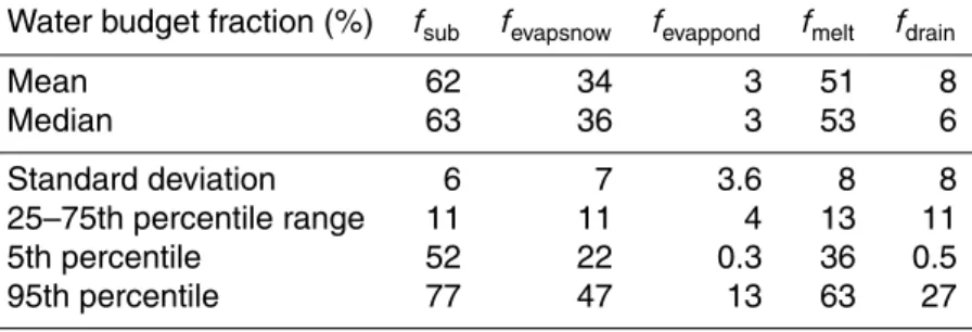
associated with upper level cold air advection from the north and strong surface cool-ing. During the day on 18 February, upper level clouds were associated with westerly flow while high humidity air at lower altitudes was associated with southerly advection. Fresh snowfall began at around 05:00 p.m. local time on 18 February and ended the experiment. Figure 3 shows time-height cross sections of temperature, wind speed, 20

water mixing ratio (q),δD and CO2mixing ratio. Time series of specific humidity, δD

and CO₂mixing ratio at the surface and at 300 m are shown on Fig. 4.

At the top of the tower, both specific humidity andδD increase during the afternoon on 17 February (Fig. 4), and signifies a shift of the air mass. The isotopic signature of this transition is characterized further using the location of the observedq,δD pair on 25

(15)

ACPD

12, 16327–16375, 2012

D. Noone et al.

Title Page

Tables Figures

◭ ◮

Back Close

Full Screen / Esc

Discussion

P

a

per

|

Dis

cussion

P

a

per

|

Discussion

P

a

per

|

Discussio

n

P

a

per

|

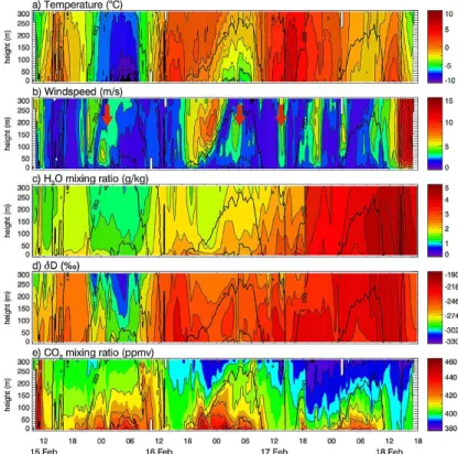
the isotopic ratios (Noone, 2012). The data show evidence of two distinct moisture pathways. The difference in the two populations of observations is expected from the change in the synoptic flow to the west and south on 18 February. For most of the experiment, the values remain close to a single coherent area of the phase diagram clustered around a line that is consistent with a saturated Rayleigh distillation (i.e., a 5

pseudoadiabatic processes) from a oceanic moisture source at 10◦C and 70 % relative humidity (purple curve). At the end of the experiment the air mass associated with the snowfall on the 18 February lies on a Rayleigh curve drawn with a saturated ocean source at around 25◦C (solid cyan curve). A model in which the precipitation efficiency is 0.5 (dashed cyan curve, see Noone 2012) captures the values early in the onset 10

of the storm. The transition between the two air masses is well described by a mixing line constrained on the upper end with an end member of −90 ‰, which is typical for wintertime precipitation in the region (e.g., Araguas-Araguas et al., 2000). These curves were chosen to provide qualitative context.

The evolution of δD during the snow storm on 18 February has two components. 15

First, enrichment is associated with the air mass change to the westerly flow in the morning (as noted above). Then, a strong depletion is associated with strong vertical mixing involving the entire troposphere in frontal systems and is accompanied by high wind speed in the final hours of the experiment (Fig. 3).

3.2 Diurnal evolution 20

Many salient features observed are related to the diurnal cycle. Figure 4 shows hu-midity at both the surface and 300 m decrease linearly throughout the first two nights, accompanied by a similar steady linear decrease ofδD values. On the first night this is associated with stable subsidence and the second night this is associated with the formation of a low level jet (LLJ). At night, surface CO2mixing ratio increase with time

25

(16)

ACPD

12, 16327–16375, 2012

D. Noone et al.

Title Page

Tables Figures

◭ ◮

Back Close

Full Screen / Esc

Discussion

P

a

per

|

Dis

cussion

P

a

per

|

Discussion

P

a

per

|

Discussio

n

P

a

per

|

the morning, specific humidity andδD values increase due to the surface latent heat flux and the growth of a convective boundary layer allows ventilation of near-surface air with low CO2 and lowδD air entrained into the boundary layer from the troposphere.

In the evening, water vapor mixing ratio andδD decreases at 300 m once thermally driven convection terminates which stops the steady input of surface water of highδD. 5

The surface source of highδD vapor does not cease immediately in the evening but becomes trapped within the growing stable boundary layer and does not reach 300 m. Two-hour averaged δD profiles are shown in Fig. 6 for different times of day that illustrate the evolution of the profile in the cases anticipated from Fig. 1. In the morning, sublimation of snow increases the humidity andδD in the boundary layer. During the 10

night the boundary layer attains lower δD values associated with air entering from above (Fig. 6a). Evidence for an evaporative source is seen in theδD as a maximum near the surface (Fig. 6b). This moist and enriched anomaly propagates quickly upward due to the strong mixing that accompanies the steadily growing convective boundary layer (Figs. 3 and 6b). The CO2, water vapor andδD all show reduced vertical gradients

15

during the day associated with strong mixing driven by solar heating (Fig. 3). In the meantime, mixing within the boundary layer and with the free troposphere allows the night time CO2maximum to dissipate.

3.3 Evolution of turbulence properties

Since highδD water vapor is emitted at the surface during the day and CO2is emitted

20

at the surface is trapped during the night,δD and CO2are complementary tracers that

reveal information about boundary layer mixing processes. For stationary boundary layers, the relative role of mixing within the boundary layer, and between the boundary layer and the free troposphere, can be exposed on the basis of mixing that follows a mixing-length hypothesis. However, when the boundary layer is heterogeneous or 25

(17)

ACPD

12, 16327–16375, 2012

D. Noone et al.

Title Page

Tables Figures

◭ ◮

Back Close

Full Screen / Esc

Discussion

P

a

per

|

Dis

cussion

P

a

per

|

Discussion

P

a

per

|

Discussio

n

P

a

per

|

Figure 3 reveals periods when δD and CO2 both feature sudden and large

varia-tions. During the night in particular, both tracers reveal the slow mixing is punctuated by bursts within the boundary layer or originating at the top of the observed profile. Such intermittent dynamical processes that affect the momentum and heat balance of the nocturnal boundary layer structure have been noticed in previous studies (Poulos et 5

al., 2002; Salmond and McKendry, 2005). An example of the influence of these events on trace gases is seen at 10:00 p.m. on 15 February:δD and CO₂suddenly decrease at 300 m and within the profile, suggesting a turbulent burst that leads to enhanced ex-change with the free troposphere. Subsequently,δD decreases while CO2 increases,

suggesting a turbulent burst within the boundary layer that mixes depletedδD down-10

ward and transports the high CO₂concentration upward, or from a lateral source. This type of transient dynamical feature is not characterized by a mixing line analysis.

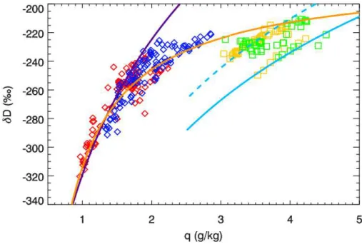
The formation of a LLJ during the second night is a sustained dynamical structure that is also not resolved by mixing line analysis. LLJs can result from many generation mechanisms. In this case, the very stable conditions, evident in both the tower data 15

(Fig. 3a) and from the TLS (Fig. 7), tends to extinguish turbulence above the typically thin surface boundary layer, which leads to unbalanced horizontal pressure gradients that accelerates the flow until turbulence is reestablished (e.g., Businger, 1973). Figure 7 shows a series of very high resolution profiles during the time of the LLJ from the TLS. The turbulence profiles show the 10–15 m deep surface layer. Before the jet appears, 20

the boundary layer profiles (the first seven profiles in Fig. 7) show a steep inversion near in the lowest 15 m that indicates the depth of the surface layer, while the structure above is near neutral. The jet appears at 21:05 LT as a result of the enhanced stability. The gas tracers show that boundary layer air is replaced by well mixed air mass advected in by the jet above the surface layer, while air below the height of the jet retains CO2

25

(18)

ACPD

12, 16327–16375, 2012

D. Noone et al.

Title Page

Tables Figures

◭ ◮

Back Close

Full Screen / Esc

Discussion

P

a

per

|

Dis

cussion

P

a

per

|

Discussion

P

a

per

|

Discussio

n

P

a

per

|

turbulent boundary layer extends up to about 150 m. When the jet disappears, CO₂and qare transported upward again at the slow rate governed by the nighttime stability.

The advective influences of the LLJ on the moisture profile would invalidate the con-ditions required for the isotope GML to be useful. The impact of a similar advective influence on the profile is illustrated well by the arrival of the frontal air mass in the 5

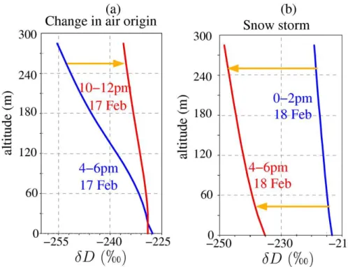
evening of the 17 February (Fig. 8a). While reminiscent of the conceptual depiction in Fig. 1c, the vertical structure is not governed by a mixing process and so is not well modeled with a mixing line. Similarly, changes in the air mass over the depth of the profiles associated with the passage of the front on the 18th (Fig. 8b) are not captured by a mixing line analysis. Under these types of advective conditions the gradient mixing 10

line approach may be valid in the surface layer where the surface exchange dominates, but transient and dynamic phenomenon are not readily accounted for in a simple tracer mixing line analysis over different sections of the full 300 m profile. On the other hand, the isotopic information is useful in identifying these dynamic changes since they do not conform to a simple mixing hypothesis.

15

3.4 Surface flux composition from mixing lines

Estimates of the δD of surface fluxes associated with evaporation and sublimation (i.e.,δDF) are obtained from the observed vertical profiles using a mixing line approach.

The temporal mixing line (TML) analysis applied on temporal series in windows of 3.5 h of data taken from any single height yields noisy results and values ofδDFthat are not

20

bounded byδD values of the snow and so appear unphysical. Testing different tempo-ral windows from 1 to 6 h, applying smoothing filters and using different heights failed to produce results that could be deemed reliable without a priori knowledge of the flux. This demonstrates that even over the time scale of a few hours, the dynamic and non-stationary nature of the boundary layer (illustrated in the previous section) violates the 25

(19)

ACPD

12, 16327–16375, 2012

D. Noone et al.

Title Page

Tables Figures

◭ ◮

Back Close

Full Screen / Esc

Discussion

P

a

per

|

Dis

cussion

P

a

per

|

Discussion

P

a

per

|

Discussio

n

P

a

per

|

Figure 9a (green), shows flux values derived from the surface (10 m, and within the surface layer), which appear to be the most reliable because it is closest to the source and because the dynamics of the surface layer are simpler than the rest of the bound-ary layer. Uncertainty is shown in Fig. 9b as the standard deviation derived from the quadrature sum of precision of the measurement, uncertainty in all steps of the calibra-5

tion and the estimate on the mixing line regression. The latter dominates. Uncertainties inδD are associated with measurement precision are±5 ‰ at 1 g kg−1and uncertain-ties arising from memory effects are typically±2 ‰. This shows that while the TML method is not generally appropriate for boundary layer data, time series data obtained from short towers may be useful. This result suggests that studies using cryogenic 10

methods to obtain samples that integrate over 10s of minutes to hours may be reliable when the conditions are chosen carefully.

The GML approach applied on profiles in the surface layer (taken from 0 to 60 m, Fig. 9 blue) yields values ofδDFat noon and in the afternoon that remain between the

predictedδD of snow sublimation and the predictedδD of evaporation of snow melt. It 15

also captures the composition of the frost sample on the morning of 18 February. Dur-ing other periods however, estimated δDF seems unphysical. This was most notable

for the case of the frost event as the surface flux changes sign from upward during the day to downward at night in association with the frost. Similar limitations can be ex-pected when the flux is small. The gradient mixing approach is sensitive to the height 20

over which the mixing line is plotted. For instance, when calculated from 0 to 300 m, the approach yields significantly higherδDF values. The results show that while the GML

method has advantages over the TML method it is not without limitations. The reason for some of the limitations and for the sensitivity to profile height warrants discussion.

The gradient mixing line approach requires a stationary profile. Most of the time, 25

(20)

ACPD

12, 16327–16375, 2012

D. Noone et al.

Title Page

Tables Figures

◭ ◮

Back Close

Full Screen / Esc

Discussion

P

a

per

|

Dis

cussion

P

a

per

|

Discussion

P

a

per

|

Discussio

n

P

a

per

|

red). The observed linear relationship suggests that the state is stationary, and explains the small sensitivity to profile height. This increases the confidence one may have in the δDF estimate. In contrast, later in the day, surface fluxes shift from sublimation

to evaporation from standing surface liquid water, so that the surface end member varies with time. This transition leads to curvature of the mixing line in the evening 5

(Fig. 10b, red). This explains why theδDF estimated from the full profiles are higher,

and are probably larger than the trueδDF value. Changes in the free tropospheric end

member associated with shifts in synoptic-scale moisture origin similarly complicate the interpretation of the mixing line.

Figure 11 illustrates the behavior of mixing lines in the morning. During the night, 10

the mixing line follows the same trajectory as that from the previous day and thus reflects the previousday’s surface fluxes (Fig. 11a, black). When frost forms, however, the mixing line follows a new slope near the surface, which leads to curvature when the full profile is considered (Fig. 11a, red). This explains the particularly low estimates ofδDF in the morning of 16, 17 and 18 February. These values do not represent the

15

δD value of frost, but rather reflect the shift from one mixing line to another. When frost formation is stronger (relative to the mixing timescale) and dominates the profile, a new stationary mixing line is established and reflects frost formation very near the surface (Fig. 11b). Indeed the gradient mixing line approach applied to the bottom 60 m (i.e., the surface layer) can resolve the isotope ratio of frost early on 18 February.

20

3.5 Bounds on attribution of surface water flux

Surface snowδD is observed to increase by about 20 ‰ every day, and decrease dur-ing the night (Fig. 9). Since evaporative enrichment of pond water, enrichment durdur-ing sublimation and re-equilibration of the snow pack with liquid give surface fluxes of dif-ferent isotope ratio, the relevant processes can be constrained with the observedδDF

25

(21)

ACPD

12, 16327–16375, 2012

D. Noone et al.

Title Page

Tables Figures

◭ ◮

Back Close

Full Screen / Esc

Discussion

P

a

per

|

Dis

cussion

P

a

per

|

Discussion

P

a

per

|

Discussio

n

P

a

per

|

to the observed values ofδDc=−175 ‰ andδD=−255 ‰ respectively. The

observa-tional constraints are typicalδD values observed on 16 and 17 February at 06:00 p.m.: δDl=−140±3 ‰ for ponds,δDc=−155±3 ‰ for snow andδDF=−220±15 ‰.

Sim-ulations were selected as plausible when the results were within one standard deviation of the observations. The mean of the ensemble of plausible solutions provides a mea-5

sure of the most likely partitioning of fluxes, and the standard deviation and confidence intervals based on percentile bins provides an estimate of the uncertainty. Table 1 sum-marizes the results for each model parameter.

Simulation results show that both evaporative enrichment and re-equilibration with melt water are necessary to explain the observed approximate 20 ‰ enrichment of the 10

snow each date. The role of snow re-equilibration is supported by observable changes in physical properties of snow over the course of the experiment from a “powder” con-sistency to a larger grained and icier structure. This is consistent with significant melting and recrystallization.

Despite the wide range of possible values for the six model parameters, the set 15

which produce simulations that match the observations depict a very consistent set of processes controlling the surface water budget (Fig. 12). Sublimation accounts for 70 to 73 % of the total surface water fluxes over the day, and for 59 to 60 % of the total snow loss. Snow samples contain 13 to 21 % of water that is refrozen liquid. The observed decrease of snow δD in the evening can be explained by drainage of evaporatively 20

enriched liquid water that had accumulated within the snow pack during the day, but this is not resolved in the calculation.

A series of eight sensitivity experiments is used to test the importance of (1) the uncertainty in the observational constraints and (2) assumptions about the isotopic model on the resulting partitioning estimate. The sensitivity to observational uncertainty 25

(22)

ACPD

12, 16327–16375, 2012

D. Noone et al.

Title Page

Tables Figures

◭ ◮

Back Close

Full Screen / Esc

Discussion

P

a

per

|

Dis

cussion

P

a

per

|

Discussion

P

a

per

|

Discussio

n

P

a

per

|

range. Values shown in the table that are higher than one show where the possible range of values has increased, and values lower than one show that the uncertainty has decreased.

The sensitivity tests show that (1) theδDF constraint does not influence the

uncer-tainty because it is itself uncertain, (2) the snowδD is the most significant constraint, 5

and (3) when the pond waterδD constraint is not used the uncertainty in the drainage fraction and pond evaporation is larger. The uncertainty of each of δDF, δD of snow

andδD of pond water was reduced by a factor of two (tests 4, 5 and 6) and shows that there is only moderate change in the uncertainty on the final partitioning fractions which suggests that the measurement capabilities are sufficient. The importance of fraction-10

ation during sublimation is tested by allowing the fractionation during sublimation to vary between the model default value of 0 ‰ (e.g., Jouzel et al., 1987; Hoffmann et al., 1998) to 40 ‰ (the maximum value observed in laboratory experiments under windy conditions, Ekaykin et al., 2009). Adding this extra degree of freedom yields signifi-cantly larger uncertainty in the estimate of the partitioning. The degree of fractionation 15

during sublimation is better constrained if the estimate ofδDFis better, as illustrated by

test 8 in which sublimation is allowed and the uncertainty ofδD_F is reduced by a factor of two.

The suite of sensitivity tests shows that the strongest constraint on the model of the snow pack is offered by measurements of the isotopic composition of the snow 20

pack itself, and that uncertainty in the estimate of the partitioning between evaporation from liquid in the snow versus sublimation is much larger with only the estimate of the net flux. Because of this, the assumption on the existence of fractionation during sublimating becomes an important aspect in obtaining robust estimates of the partition fractions.

(23)

ACPD

12, 16327–16375, 2012

D. Noone et al.

Title Page

Tables Figures

◭ ◮

Back Close

Full Screen / Esc

Discussion

P

a

per

|

Dis

cussion

P

a

per

|

Discussion

P

a

per

|

Discussio

n

P

a

per

|

4 Conclusions

Measurements of the lower boundary layer vertical profiles of specific humidity and the hydrogen isotope ratio of water vapor were made from a 300 m tall tower every 15 min during four winter days in Colorado. At the synoptic scale, the isotopic evolution reflects the origin and differing hydrologic histories of air masses. At the daily scale, the 5

evolution of the isotope ratio reflects the sublimation of snow, evaporation of ponds and strong boundary layer mixing during the day. Since water vapor sources are largest and positive during the day and CO2 is emitted at the surface is trapped at night, they are

complementary tracers of boundary layer mixing. Together, they show strong vertical mixing during the day and a shallow well stratified boundary layer during the night, in 10

which mixing occurs mainly through intermittent bursts of turbulence.

Several approaches were employed to deduce the isotope ratio of the flux using a mixing line analysis. Mixing line analyses applied to time series data yield very noisy results, due to the non-stationary and diverse set of processes (e.g., evaporation, turbu-lent mixing, slow shifts in tropospheric composition, etc.) taking place over the duration 15

of the sections of data. Mixing lines constructed from vertical profiles yield more physi-cally satisfying results during the day when thermal convection is well established, and the mixing line estimates from the surface layer (up to a few 10s of meters) provide the most reliable estimates. This confirms that measurements from short (10 m) towers are beneficial, but there remains a need for careful analysis of the gradient method. 20

The profile above the surface layer is influenced by more complex dynamics, and cap-tures processes and source other than those associated with surface exchange, which negates the assumptions underlying the mixing model. The gradient mixing line ap-proach is also able to capture some frost formation events before sunrise. However, it fails during the night and every time the profiles deviate significantly from station-25

(24)

ACPD

12, 16327–16375, 2012

D. Noone et al.

Title Page

Tables Figures

◭ ◮

Back Close

Full Screen / Esc

Discussion

P

a

per

|

Dis

cussion

P

a

per

|

Discussion

P

a

per

|

Discussio

n

P

a

per

|

suggests a shift from snow sublimation in the morning to pond evaporation through the day, which provides the evidence for physical changes in the characteristics of the source and a constraint for quantitative attribution.

Although limitations in mixing line analysis have been revealed at the processes level, the use of an optimal estimation approach allows synthesis of uncertain data from 5

multiple sources with an adequate forward mass balance model to form an estimate of the flux partitioning. This is an important advance in the source attribution problem because it sets a path for more formal assimilation of surface isotopic data into detailed process models to constrain surface water and energy balance rather than relying on simple mixing methods. Additional information on water vapor source and exchange 10

processes is provided by combiningδD andδ18O, i.e., from deuterium excess mea-surements (e.g., Gat and Matsui, 1991). Developing appropriate calibration procedures for water vapor isotope ratio measurements remains a challenge, especially for deu-terium excess when the humidity is low and highly variable as is typical in field settings. The analysis shows that while vapor measurements are important, measurements of 15

the possible source reservoirs (especially soil water, snow pack, standing liquid and potentially precipitation, etc.) offer stronger constraints. These should be considered essential in developing observational programs that seek to use isotopic data for flux attribution.

Appendix A 20

Calibration of isotopic measurements

Raw δ (both D and 18O) measurements are corrected to remove measurement de-pendence on mixing ratio and calibrated to the standard scale as shown schematically in Fig. 13. Calibration is based on data obtained from discrete injections of five known standards with a PAL autosampler and the Picarro vaporizer unit. Injections were made 25

(25)

ACPD

12, 16327–16375, 2012

D. Noone et al.

Title Page

Tables Figures

◭ ◮

Back Close

Full Screen / Esc

Discussion

P

a

per

|

Dis

cussion

P

a

per

|

Discussion

P

a

per

|

Discussio

n

P

a

per

|

syringe for 6.20 and 12.4, and a 500 nl syringe for lower mixing ratios). Standard waters from Florida, Boulder, and the West Antarctic Ice Sheet, Greenland and Vostok were supplied by the University of Colorado Stable isotope Laboratory and tied to SMOW-SLAP scale using IAEA primary standards. Humidity dependence is characterized by fitting a function, f, to measured values. Various functions can be used (geometric, 5

splines, polynomials, etc.), and here we choose a cubic polynomial in the formδ=f(x) wherexis the natural logarithm ofq. The fit accounts for uncertainty in theδandq us-ing a Monte Carlo approach. The shape of the curve depends weakly on theδvalue of the standard water, which is accounted for by linearly interpolating the regression coef-ficients between the knownδ values of the standard water and the measuredδvalue. 10

The humidity correction is the difference between the δ value at the measurement q value and theδvalue at a reference value taken asqref=6.2 g kg−

1

(Fig. 13a). Adjust-ment to the SMOW-SLAP scale is achieved with a quadratic fit between the values of standard waters known from mass spectrometer measurement and the measurements of those standard waters with the spectroscopic analyzer (Fig. 13b). A quadratic fit is 15

needed to remove the non-linearity that would otherwise introduce errors of 2.8 ‰ for δD and 0.15 ‰ forδ18O.

Uncertainty associated with instrument precision (which is a function of humidity), re-peatability in measurement of standard waters, uncertainty in regression and curve fit-ting coefficients and accuracy of calibration waters is propagated though the approach 20

using a Monte Carlo method to give an estimate on the measurement accuracy. The Monte Carlo ensemble is constructed by perturbing all quantities involved in the cali-bration by a normally distributed random amount proportional to one standard deviation of each quantity. The Monte Carlo ensemble has 10 000 members for each measured value, and the mean and standard deviation of the ensemble provides the estimate of 25

(26)

ACPD

12, 16327–16375, 2012

D. Noone et al.

Title Page

Tables Figures

◭ ◮

Back Close

Full Screen / Esc

Discussion

P

a

per

|

Dis

cussion

P

a

per

|

Discussion

P

a

per

|

Discussio

n

P

a

per

|

forδD, and 1.0 to 0.30 ‰ for δ18O over the observed range of q. The precision of q measurements is 2 %.

Appendix B

Algorithm for memory correction

Because of significant memory effects associated with low flow rates (30 cc min−1), the 5

volume of the inlet and sample lines and instrument effects, the calibratedδprofiles for upward and downward motions of the elevator are different, and need to be reconciled by a posterior correction. Downward profiles haveδvalues typically 9.1±9.5 ‰ lower than the upward profiles. This is because downward profiles retain the memory of the depleted vapor encountered at the top of the tower, whereas upward profiles retain the 10

memory of enriched vapor encountered at the surface.

It is assumed that at each measurement timet, the composition of the vapor inside the isotopic analyzer,δobs(t), is a combination of new sample vapor and the vapor from

previous observations, and that the vapor is mixed with a time constantτ. The value ofτ accounts for both the time required for mixing and the time scale of interactions 15

between water molecules and all internal surfaces. Each vapor measurement reflects the environment vapor with a lag of∆tlagdue to the transport time in the inlet. At each

timet,δobs is expressed as

δobs(t)=

1−∆t

τ

δobs(t−∆t)+

∆t τ

δenv(t−∆tlag) (B1)

whereδenv is theδ value of the environment and∆tis the time interval between

mea-20

surements. Bothτand∆tlagvary with time, depend on wind, humidity and temperature

(27)

ACPD

12, 16327–16375, 2012

D. Noone et al.

Title Page

Tables Figures

◭ ◮

Back Close

Full Screen / Esc

Discussion

P

a

per

|

Dis

cussion

P

a

per

|

Discussion

P

a

per

|

Discussio

n

P

a

per

|

This estimation problem is regularized under the following assumptions: (1)τ(t) and

∆tlag(t) are constant over each upward and downward motion of the elevator, (2)δenv

varies slowly enough in time for δenv to be treated as constant for each of the 156

elevator cycles (a cycle includes one up and one down), and (3) the vertical structure ofδenv(z) takes the form:

5

δenv(z)=δ0+γz+Bzrln

_z

zr

+Aexp (

−(z−zm)

2

2σ2

)

(B2)

This function is quite flexible, and allows a wide range ofδvalue profiles, with different average values, different vertical gradients, curvatures at the top or bottom, and up to two local maxima or minima. The time scale of the memory effect, of the order of several minutes, prevents statistically robust retrieval of any more detail in the profiles 10

other than those included in Eq. (13).

This leaves 11 parameters to optimize for each elevator cycle: 7 parameters for the shape ofδ_env(z) and up and down values for τ and ∆t_lag. With 11 parameters over a 300 m profile it is reasonable to conceptualize an effective resolution of approximately 27 m. Using all measurements from the δenv(t) time series for both the upward and

15

downward motions of the elevator allowsδenv(t) to be constrained efficiently.

Minimiz-ing the (root mean squared) difference between the upward and downward profiles effectively removes the memory effect. This mismatch is typically less than 2.5 ‰ for δD which is comparable in size to the measurement precision.

The procedure is applied independently toδD,δ18O andq. 20

Acknowledgements. We thank Bruce Vaughn, Valerie Morris and Jim White of the University of Colorado Stable Isotope Laboratory for providing calibration standards and invaluable advice on sample preparation and laboratory isotopic analysis. We thank Chris Still of University of Cal-ifornia at Santa Barbara and Brent Helliker of Penn State for advice on design of the vacuum cryogenic extraction line. We are indebted to Emily Graham and Peter Blanken of the

Depart-25

(28)

ACPD

12, 16327–16375, 2012

D. Noone et al.

Title Page

Tables Figures

◭ ◮

Back Close

Full Screen / Esc

Discussion

P

a

per

|

Dis

cussion

P

a

per

|

Discussion

P

a

per

|

Discussio

n

P

a

per

|

Career program (AGS-0955841), NASA Atmospheric Composition Program (NNX08AR23G), a grant from the NASA Jet Propulsion Laboratory and the University of Colorado Undergraduate Research Opportunities Program.

References

Angert, A., Lee, J. E., and Yakir, D.: Seasonal variations in the isotopic composition of

near-5

surface water vapour in the eastern Mediterranean, Tellus B, 60, 674–684, 2008.

Araguas-Araguas, L., Froehlich, K., and Rozanski, K.: Deuterium and oxygen-18 isotope com-position of precipitation and atmospheric moisture, Hydrol. Process., 14, 1341–1355, 2000. Avissar, R. and Werth, D.: Global hydroclimatological teleconnections resulting from tropical

deforestation, J. Hydrometeorol., 6, 134–145, 2005.

10

Balsley, B. B., Jensen, M. L., and Frehlich, R. G.: The use of state-of-the-art kites for profiling the lower atmosphere, Bound.-Lay. Meteorol., 87, 1–25, 1998.

Bigeleisen, J.: Statistical mechanics of isotope effects on the thermodynamic properties of con-densed systems, J. Chem. Phys., 34, 1485–1493, 1961.

Blumen, W.: An Observational Study of Instability and Turbulence in Nighttime Drainage Winds,

15

Bound.-Lay. Meteorol., 28, 245–269, 1984.

Boe, J. and Terray, L.: Uncertainties in summer evapotranspiration changes over Eu-rope and implications for regional climate change, Geophys. Res. Lett., 35, L05702, doi:10.1029/2007GL032417, 2008.

Boone, A., Habets, F., Noilhan, J., Clark, D., Dirmeyer, P., Fox, S., Gusev, Y., Haddeland, I.,

20

Koster, R., Lohmann, D., Mahanama, S., Mitchell, K., Nasonova, O., Niu, G. Y., Pitman, A., Polcher, J., Shmakin, A. B., Tanaka, K., van den Hurk, B., Verant, S., Verseghy, D., Viterbo, P., and Yang, Z. L.: The Rhone-aggregation land surface scheme intercomparison project: An overview, J. Climate, 17, 187–208, 2004.

Bosilovich, M. G. and Chern, J. D.: Simulation of water sources and precipitation recycling for

25

the MacKenzie, Mississippi, and Amazon River basins, J. Hydrometeorol., 7, 312–329, 2006. Brown, S. S., Dub ´e, W. P., Osthoff, H. D., Wolfe, D. E., Angevine, W. M., and Ravishankara, A.