CAMPUS DE ILHA SOLTEIRA
SIDNEY BRUCE SHIKI
APPLICATION OF VOLTERRA SERIES IN NONLINEAR
MECHANICAL SYSTEM IDENTIFICATION AND IN STRUCTURAL HEALTH MONITORING PROBLEMS
APPLICATION OF VOLTERRA SERIES IN NONLINEAR
MECHANICAL SYSTEM IDENTIFICATION AND IN STRUCTURAL HEALTH MONITORING PROBLEMS
Thesis presented to the Faculdade de Enge-nharia de Ilha Solteira - UNESP as a part of the requirements for obtaining the Doctorate in Mechanical Engineering.
Knowledge area: Solid Mechanics.
Prof. Dr. Samuel da Silva Advisor
Prof. Dr. Gaëtan Kerschen Co-advisor
. .
FICHA CATALOGRÁFICA
Desenvolvido pelo Serviço Técnico de Biblioteca e Documentação
Shiki, Sidney Bruce.
Application of Volterra series in nonlinear mechanical system identification and in structural health monitoring problems / Sidney Bruce Shiki. -- Ilha Solteira: [s.n.], 2016
114 f. : il.
Tese (doutorado) - Universidade Estadual Paulista. Faculdade de Engenharia de Ilha Solteira. Área de conhecimento: Mecânica dos Sólidos, 2016
Orientador: Samuel da Silva Co-orientador: Gaëtan Kerschen Inclui bibliografia
1. Nonlinear structures. 2. Structural health monitoring. 3. Volterra models. 4. Kautz filters. 5. Nonlinear model updating.
I would like to thank Prof. Samuel da Silva for almost 6 years of orientation and friendship since when I was an undergraduate student at Foz do Iguaçu. The dedication given by Prof. Samuel is one of the big reasons for me to pursue the academic life.
To Profs. Vicente Lopes Junior, Michael J. Brennan and João Antonio Pereira from UNESP who contributed to this thesis with many advices and questions.
To Profs. Gaëtan Kerschen (Université de Liège) and Michael D. Todd (University of California, San Diego) for the valuable period of research internship in their laboratories and the many comments and perspectives about my research.
To my girlfriend Giselle who gave me more than 7 years of unconditional support for me to pursue my dreams even when I needed to be far. Her affection and care were fundamental for me to reach my goals.
To my mother Ilda and all my family that always supported me to study hard and go after the best opportunities in my life.
To my friends from the "República" Cristian, Oscar and Vinícius for the friendship in the good and the tough times during the doctorate studies. All the the breaks for coffees and talks were necessary to keep our minds in a stable state.
To the technician from UNESP Carlos Santana and to my friend and colleague Cris-tian Hansen who gave me a lot of help during the experimental tests used in this thesis.
To all my colleagues from the Group of Intelligent Materials and Systems (GMSINT), the Mechanical Engineering Department and to all the technical staff from UNESP.
I would also like to thank the São Paulo Research Foundation (FAPESP) who pro-vided financial support for my master degree (grant number 2012/04757-6I), direct docto-rate (grant number 2013/25148-0II) and during my research internship abroad in Belgium (grant number 2012/21195-1III) and in the United States (grant number 2015/03560-2IV).
I
http://www.bv.fapesp.br/pt/bolsas/134447
II
http://www.bv.fapesp.br/pt/bolsas/149957
III
http://www.bv.fapesp.br/pt/bolsas/139239
IV
and Technological Development (CNPq, grant number 470582/2012-0) which provided resources for the participation in conferences and also equipments for the experiments during the thesis. Finally the author also thank CNPq and the Fundação de Amparo à Pesquisa do Estado de Minas Gerais (FAPEMIG) for partially funding the research through the National Institute of Science and Technology in Smart Structures in Engi-neering (INCT-EIE).
V
did not have some inkling of this through observations could ever have imagined such a marvel as nature is.
Nonlinear structures are frequent in structural dynamics, specially considering screwed components, with joints, clearance or flexible components presenting large displacements. In this sense the monitoring of systems based on classical linear methods, as the ones based on modal parameters, can drastically fail to characterize nonlinear effects. This thesis proposed the use of Volterra series for nonlinear system identification aiming appli-cations in damage detection and parameter quantification. The property of this model of representing the linear and nonlinear components of the response of a system was used to formulate damage features to make clear the need of nonlinear modeling. Also metrics based on the linear and nonlinear residues of the terms of the Volterra model were em-ployed to identify parametric models of the structure. The proposed methodologies are illustrated in experimental setups to show the relevance of nonlinear phenomena in the structural health monitoring.
Estruturas com comportamento não-linear são frequentes em dinâmica estrutural, principalmente considerando componentes parafusados, com juntas, folgas ou estruturas flexíveis sujeitas à grandes deslocamentos. Desse modo, o monitoramento de estruturas com métodos lineares clássicos, como os baseados em parâmetros modais, podem falhar drasticamente em caracterizar efeitos não-lineares. Neste trabalho foi proposta a uti-lização de séries de Volterra para identificação de sistemas mecânicos não-lineares em aplicações de detecção de danos e quantificação de parâmetros. A propriedade deste modelo de representar separadamente os componentes de resposta linear e não-linear do sistema foi aplicada para se construir índices de dano que evidenciam a necessidade de modelagem não-linear. Além disso métricas de resíduo linear e não-linear dos termos do modelo de Volterra são empregadas para identificar modelos paramétricos da estrutura. As metodologias propostas são ilustradas em bancadas experimentais de modo a eviden-ciar a importância de fenômenos não-lineares para o monitoramento de estruturas.
a1 - Parameter of the β function a2 - Parameter of the β function
bη - Parameter of the Kautz orthonormal function c - Damping coefficient
dη - Parameter of the Kautz orthonormal function eη - Prediction error of order η
eη,ref - Prediction error of order η in the reference condition eη,unk - Prediction error of order η in the unknown condition f - Input force
H0 - Null hypothesis
H1 - Alternative hypothesis
h1 - First-order Volterra kernel in the continuous-time formulation h2 - Second-order Volterra kernel in the continuous-time formulation h3 - Third-order Volterra kernel in the continuous-time formulation hη - η−order Volterra kernel in the continuous-time formulation
J1 - Number of orthonormal functions to represent the first Volterra kernel J2 - Number of orthonormal functions to represent the second Volterra
ker-nel
J3 - Number of orthonormal functions to represent the third Volterra kernel Jη - Number of orthonormal functions to represent theη−thVolterra kernel k - Sample number for the discrete-time formulation in the Volterra series k1 - Linear stiffness
k2 - Quadratic stiffness k3 - Cubic stiffness
lη,ij - Input signal filtered by the orthonormal function
m - Mass coefficient
N1 - Memory length of the first Volterra kernel in the discrete-time formula-tion
N2 - Memory length of the second Volterra kernel in the discrete-time for-mulation
n1 - First-order sample delay in the discrete-time formulation of Volterra series
n2 - Second-order sample delay in the discrete-time formulation of Volterra series
n3 - Third-order sample delay in the discrete-time formulation of Volterra series
nη - η-order sample delay in the discrete-time formulation of Volterra series P - Probability density function of the λη damage index
p - Vector with the parameters to be found p - Probability value of the distribution (p-value) T - transpose of a matrix
t - Continuous time variable
u - Input signal applied in the Volterra series V - maximum number of used orthonormal filters
v1 - Number of degrees of freedom for the prediction error in the unknown condition
v2 - Number of degrees of freedom for the prediction error in the reference condition
x - Displacement of the Duffing oscillator ˙
x - Velocity of the Duffing oscillator ¨
x - Acceleration of the Duffing oscillator
y - Vector with the total output of the Volterra series y1 - Vector with the first-order output of the Volterra series y2 - Vector with the second-order output of the Volterra series y3 - Vector with the third-order output of the Volterra series y - Total output of the Volterra series
yexp - Experimentally measured response y1 - First-order output of the Volterra series y2 - Second-order output of the Volterra series y3 - Third-order output of the Volterra series yη - η−order output of the Volterra series
B
B2 - Second-order Volterra kernel in the orthonormal basis
B2,ref - Reference second-order Volterra kernel in the orthonormal basis
B3 - Third-order Volterra kernel in the orthonormal basis
B3,ref - Reference third-order Volterra kernel in the orthonormal basis
Bη - η−order Volterra kernel in the orthonormal basis
Clin - Linear objective function for parameter identification
Cnlin - Nonlinear objective function for parameter identification
H1 - First-order Volterra kernel in the discrete-time formulation
H2 - Second-order Volterra kernel in the discrete-time formulation
H3 - Third-order Volterra kernel in the discrete-time formulation
Hη - η−order Volterra kernel in the discrete-time formulation
Sη - Pole representing the Kautz functions in the continuous frequency do-main
Zη - Pole representing the Kautz functions in the discrete frequency domain ¯
Zη - Conjugate of the pole representing the Kautz functions in the discrete frequency domain
Greek letters
α - Significance value of the hypothesis test Γ - Matrix with combinations of the input signal
Γ1 - Matrix with combinations of the input signal for the first-order output Γ2 - Matrix with combinations of the input signal for the second-order
out-put
Γ3 - Matrix with combinations of the input signal for the third-order output ζ1 - Damping ratio representing the first Volterra kernel in the orthonormal
basis
ζ2 - Damping ratio representing the second Volterra kernel in the orthonor-mal basis
λ2 - Damage index of second-order λ3 - Damage index of third-order λη - Damage index of order η
ξ - Damping ratio of the Duffing oscillator σ - Standard deviation operator
τ1 - Time delay for the first Volterra kernel in the continuous-time formula-tion
τ2 - Time delay for the second Volterra kernel in the continuous-time for-mulation
τ3 - Time delay for the third Volterra kernel in the continuous-time formu-lation
τη - Time delay for theη−th Volterra kernel in the continuous-time formu-lation
Φ - Vector with the considered Volterra kernels Φ1 - Vector with the first Volterra kernel
Φ2 - Vector with the second Volterra kernel Φ3 - Vector with the third Volterra kernel
ψ - Orthonormal function in the discrete-time domain Ψ - Orthonormal function in the discrete frequency domain
ω1 - Frequency representing the first Volterra kernel in the orthonormal ba-sis
ω2 - Frequency representing the second Volterra kernel in the orthonormal basis
CDF - Cumulative distribution function FRF - Frequency response function GVT - Ground vibration testing HBM - Harmonic balance method
HOFRF - Higher-order frequency response function LANL - Los Alamos National Laboratory
MIMO - Multiple inputs/multiple outputs
NOFRF - Nonlinear output frequency response function PDF - Probability density function
PSD - Power spectral density RMS - Root mean square
ROC - Receiver operating characteristic SHM - Structural health monitoring SIMO - Single input/multiple outputs SISO - Single input/single output
1 Flowchart showing the methodology for the identification of Volterra models. 41 2 Detection of nonlinearity in the Duffing oscillator. The continuous line
is the low input (0.1 N), -△- is the medium input (0.3 N) and -○- is the high input (0.5 N). . . 42 3 Convergence analysis of the Volterra model representing the Duffing
oscil-lator. . . 43 4 Illustration of the first Volterra kernel in the physical basis representing
the Duffing oscillator. . . 45 5 Illustration of the second Volterra kernel in the physical basis representing
the Duffing oscillator. . . 45 6 Illustration of the third Volterra kernel in the physical basis representing
the Duffing oscillator. . . 46 7 Output of the identified Volterra model. The continuous line---represents
the response of the model and, ○ is the response of the Duffing oscillator. . 46 8 Components of the response to a chirp input for the Duffing oscillator. The
continuous line is the linear component (y1), is the second order nonlinear response (y2) and is the third order nonlinear response (y3). 47 9 Comparison between the Fourier series coefficients of the responses to a sine
excitation of the oscillator and the identified model. -○- is the reference
signal and -△-is the response of the Volterra model. . . 47 10 Comparison between the Fourier series coefficients of the response
compo-nents to a sine excitation. -△- is the linear component, -Ԃ- is the second
14 Experimental setup of the magneto-elastic system. . . 61
15 Detection of nonlinearity in the magneto-elastic system. The continuous line is the low input (0.01 V), -△- is the medium input (0.10 V) and -○- is the high input (0.15 V). . . 62
16 Convergence analysis of the Volterra model representing the magneto-elastic system. . . 63
17 Identified Volterra kernels representing the magneto-elastic system. The continuous line is the normalized 1st kernel (H 1/∣∣H1∣∣), is the normalized main diagonal of the 2nd kernel (diag(H 2)/∣∣diag(H2)∣∣) and-○ -is the normalized main diagonal of the 3rd kernel (diag(H 3)/∣∣(diag(H3)∣∣). 65 18 Output of the identified Volterra model. The continuous line---represents the response of the model and, ○ is the response of the Duffing oscillator. . 65
19 Components of the response to a chirp input for the magneto-elastic system. The continuous line is the linear component (y1), is the second order nonlinear response (y2) and is the third order nonlinear response (y3). . . 66
20 Nonlinearity index for the magneto-elastic system. . . 66
21 Photo illustrating the GVT in the F-16 aircraft. . . 67
22 Detailed photos of the GVT in the F-16 fight aircraft. . . 68
23 Mode shape of the F-16 aircraft subjected to nonlinear effects. . . 68
24 Time-frequency distribution of the response of the F-16 aircraft to a 15 N chirp excitation. . . 68
25 Experimental FRFs of the F-16 aircraft using a chirp input. The continuous line is the low input (5 N), -△- is the medium input (10 N) and-○-is the high input (15 N). . . 69
the model and, ○ is the measured response. . . 71 29 Output of the identified Volterra model representing the F-16 aircraft for
an input level of 15 N. The continuous line --- represents the response of the model and, ○ is the measured response. . . 71 30 Components of the output of the Volterra model representing the F-16
aircraft. The blue continuous line is the linear component (y1) and the red line is the nonlinear component (y3). . . 72 31 Time-frequency distribution of the components of the response to a chirp
excitation obtained by the Volterra model of the F-16 aircraft. . . 72 32 FRFs of the output of the Volterra kernels using a chirp input. The
con-tinuous line is the low input (5 N), -△- is the medium input (10 N) and -○- is the high input (15 N). . . 73
33 Nonlinearity index for the F-16 aircraft. . . 73 34 Illustration of the damage simulation . . . 76 35 Linear index under two different input levels. The continuous line
is representing the indexes during the damage applications (states 1 to 4) and represents the indexes during the repair (states 5 to 8). . . 77 36 Nonlinear index under two different input levels. The continuous line
is representing the indexes during the damage applications (states 1 to 4) and represents the indexes during the repair (states 5 to 8). . . 77 37 Distribution of the experimental linear damage index compared to the
the-oretical distribution. The blue bar represents the experimental data and the continuous line represents the theoretical distribution. . . 78 38 Distribution of the experimental nonlinear damage index compared to the
theoretical distribution. The blue bar represents the experimental data and the continuous line represents the theoretical distribution. . . 79 39 ROC curves of the damage indexes. -△-is the curve for the low level input
(0.05 V) and -○-has a high input level (0.10 V). . . 83
42 Experimental stepped sine response for the pre-compressed beam. The continuous line was calculated for a low input level (0.01 V),-△- has a medium input level (0.14 V) and-○- has a high input level (0.20 V). . . . 83
43 Identified Volterra kernels representing the pre-compressed beam. The continuous line is the normalized 1st kernel (H
1/∣∣H1∣∣), is the normalized main diagonal of the 2nd kernel (diag(H
2)/∣∣diag(H2)∣∣) and-○ -is the normalized main diagonal of the 3rd kernel (diag(H
3)/∣∣(diag(H3)∣∣). 85 44 Linear objective function as a function of the mass coefficient. . . 86 45 Nonlinear objective function in relationship to the k3 andζ for the medium
input level data (0.05 V). . . 87 46 Nonlinear objective function in relationship to the k3 and ζ for the high
input level data (0.10 V). . . 87 47 Output of the identified grey-box model. The continuous line
repre-sents the response of the model and, ○ is the measured response. . . 88 48 Experimental FRF for the pre-compressed beam. The continuous line
was calculated for a low input level (0.01 V), -△- has a medium input level (0.05 V) and -○-has a high input level (0.10 V). . . 88
1 Comparison between different input signals in the identification of Volterra kernels. . . 38 2 Input signal used for the identification of the Volterra kernels representing
the Duffing oscillator. . . 42 3 Optimization parameters for the calculation of the Kautz parameters in
the Duffing oscillator. . . 44 4 Information for the identification of the Kautz functions of the Duffing
oscillator. . . 44 5 Input signal used for the identification of the Volterra kernels representing
the magneto-elastic system. . . 63 6 Optimization parameters for the calculation of the Kautz parameters in
the magneto-elastic system. . . 64 7 Information for the identification of the Kautz functions of the
magneto-elastic system. . . 64 8 Input signal used for the identification of the Volterra kernels representing
the F-16 aircraft. . . 69 9 Optimization parameters for the calculation of the Kautz parameters of
the F-16 aircraft. . . 70 10 Information for the identification of the Kautz functions of the F-16 aircraft. 70 11 Structural states simulated in the nonlinear system. . . 76 12 Results of the hypothesis tests for different significance levels under low
level input (0.01 V). . . 80 13 Results of the hypothesis tests for different significance levels under high
15 Optimization parameters for the calculation of the Kautz parameters in the pre-compressed beam. . . 84 16 Information for the identification of the Kautz functions of the pre-compressed
1 Introduction 23
1.1 Motivation . . . 23 1.2 Main contributions of the thesis . . . 25 1.3 Objective . . . 26 1.4 Outline of the thesis . . . 26
2 Identification of Volterra models 28
2.1 Overview of the literature in nonlinear system identification with Volterra series . . . 28 2.2 Volterra series . . . 30 2.3 Identification of Volterra kernels . . . 33 2.4 Identification of the kernels using orthonormal functions . . . 35 2.5 Identification of the Volterra kernels for a Duffing oscillator . . . 40 2.6 Conclusions . . . 48
3 Methodologies for the application in SHM 50
3.1 Overview of the literature for nonlinear techniques in SHM . . . 50 3.2 Damage detection using Volterra series . . . 53 3.3 Parameter identification using the Volterra kernels . . . 57 3.4 Conclusions . . . 58
4 Identification of Volterra kernels in experimental examples 60
4.3 Conclusions . . . 73
5 Experimental application of Volterra series for SHM 75
5.1 Application of Volterra series in the detection of structural variations . . . 75 5.2 Parameter quantification in a nonlinear system . . . 81 5.3 Conclusions . . . 89
6 Final remarks 91
6.1 Main conclusions . . . 91 6.2 Suggestions for future works . . . 92
References 94
Appendix A - Details on the identification of Volterra kernels 103
1
Introduction
This chapter presents a brief introduction to the subject of the thesis. A motivation of the research is presented in the section 1.1. The main contributions of this thesis and the objectives of the research are presented in the sections 1.2 and 1.3, respectively. Finally, section 1.4 shows the outline of the chapters and the respective content.
1.1
Motivation
The relevance of considering nonlinear phenomena in the dynamics of structures and machines increased due to the need of better performance in terms of comfort, weight reduction, noise among other requirements (KERSCHEN et al., 2006). Nonlinear behavior can bring complex effects as jumps, limit cycle oscillations, harmonic distortion, chaos, among others even in simple academic examples as the ones described in the book of Virgin (2000). These effects can be a problem for the use of traditional techniques fundamentally based on the linear superposition principle (WORDEN; TOMLINSON, 2001) or can cause harm to the systems due to the sudden appearance of unexpected change in the structure vibration as is the case of the jump phenomenon (BRENNAN et al., 2008). On the other hand it is also possible to make use of nonlinear properties in the improvement of mechanical design. A few examples are in the use of nonlinearities for vibration isolators (KOVACIC et al., 2008) and energy harvesters (ERTURK; INMAN, 2011) aiming to improve the performance of these devices. Those cases shows both examples where one would prefer to avoid nonlinear effects and situations where these responses can improve the development of new devices.
be fully described by the following actions:
1. Identification of the presence of damage in the structure; 2. Determination of the geometric location of the damage; 3. To establish the kind of damage present;
4. Quantification of the severity of the damage;
5. Prediction of the remaining useful life of the system.
The nonlinear behavior of structures can be important in all the five steps for the damage identification process since it can change significantly the expected results in these systems. For this reason a big concern in the SHM literature is to take in account nonlinear effects in order to properly identify the damage state of a structure. In this way the nonlinear behavior in mechanical systems is treated by two main approaches (NICHOLS; TODD, 2009) where the analyst must handle with this behavior (or else
avoid it):
• First approach: nonlinearity is considered to be caused by the damage in the system; • Second approach: the systems is inherently nonlinear even before the occurrence of
the damage.
In the first approach the damage is directly related to the nonlinear behavior and the structure is considered to be linear before its occurrence. This is an appealing strategy because typical fault modes like cracks, impacts, delamination and rubbing of rotating machinery induce nonlinearity in the response of the system (NICHOLS; TODD, 2009). This situation allows to detect structural changes by identifying and characterizing the presence of nonlinear behavior in the response of the system. For this case many well-established nonlinear tools as coherence functions, Hilbert transform, higher-order spec-tra and phase-space methods can be employed (CAMBRAIA, 1990; OVERBEY; TODD, 2007; WORDEN et al., 2008). Many recent papers in the SHM literature still use this kind of approach with good results considering damage features based on modal proper-ties (BANDARA et al., 2014), wave propagation (YELVE et al., 2014) and other signal processing tools (GHAZI; BÜYÜKÖZTÜRK, 2015).
system (BORNN et al., 2010). This case demands to properly model the baseline behavior of the structure in a way that the inherent nonlinear effects of the system are not mis-takenly viewed as due to a damage. In this situation nonlinear system identification and signal processing techniques can be used to take in account nonlinear effects before the structural change. Techniques as restoring force surface method, nonlinear autoregressive models, Hilbert transform, principal component analysis, time-frequency analysis among others can be applied to identify such nonlinearity (KERSCHEN et al., 2006; WORDEN et al., 2008; BORNN et al., 2010; CHANPHENG et al., 2012; REYNDERS et al., 2013). However, there is still no general model to deal with nonlinear dynamics in a comprehen-sive way, and the application of mathematical tools in nonlinear problems tends to be case-specific (KERSCHEN et al., 2006).
In this thesis the focus will be given to problems where the system is nonlinear be-fore the occurrence of the damage. The investigation will aim to present possible ways of applications of the Volterra series expansion in the identification of the presence of the damage and quantification of parameters. This model will be used in the single in-put/single output (SISO) formulation to represent nonlinear vibrating structures. The Volterra model is identified by minimizing the output error of the series expansion with relationship to the experimental response measured in the system. The properties of this model will be used to show the needs of considering nonlinear models when monitoring structures under the nonlinear regime of motion.
1.2
Main contributions of the thesis
The main contributions of the research presented in this thesis are:
• Proposition of a methodology for the identification of discrete Volterra kernels in vibratory systems using Kautz functions;
• Utilization of the Volterra model for the detection of structural changes and in the quantification of parameters;
• Comparison between the consequences of assuming or not a nonlinear damage index under the nonlinear regime of motion in the structure;
The results of this thesis also allowed a few publications in conference and journal papers. The appendix B summarize the publications submitted during the doctorate.
1.3
Objective
To develop methodologies using Volterra series for the damage detection and parame-ter quantification aiming applications in SHM of initially nonlinear systems.
1.4
Outline of the thesis
This thesis is organized in 6 chapters and two appendices with the following content: • Chapter 1 - Introduction: shows the motivation and main objectives of the
research presented in this thesis;
• Chapter 2 - Identification of Volterra models: describe the Volterra series ex-pansion and the formulation of this model using orthonormal functions to represent the Volterra kernels. After that the procedure to make a least-squares estimation of the kernels is summarized and a simulated example of the identification of kernels is performed in a classical asymmetric Duffing oscillator;
• Chapter 3 - Methodologies for the application in SHM:introduces the reader to the proposed methodologies of application of the Volterra model as a tool for damage detection and parameter identification problems.
• Chapter 4 - Identification of Volterra kernels in experimental examples: the calculation of the Volterra kernels representing two experimental setup is pre-sented in this chapter. The first example is illustrated by a magneto-elastic system with hardening behavior. The second example is a F-16 aircraft tested during a ground vibration testing which showed softening effects in the frequency domain. With the Volterra models representing these systems it is then possible to analyze the components of the Volterra model to show the linear and nonlinear contribu-tions.
• Chapter 6 - Final remarks: this chapter presents the main final conclusions about the present thesis with proposals for further development in this research area.
• Appendix A - Details on the identification of Volterra kernels: the ap-pendix is a complement of the chapter 2 in order to have a better understanding of the Volterra series and the practical identification of the kernels.
2
Identification of Volterra models
This chapter brings the essential information to understand the methodology for the identification of a Volterra model. Additional explanation of this formulation is given in the appendix A. The section 2.1 starts with an overview of the literature available in the subject of nonlinear system identification, specially in the applications with Volterra series in mechanical systems. The Volterra series formulation is presented in the section 2.2. Sections 2.3 and 2.4 shows the method for the calculation of the kernels of the Volterra model and the orthonormal representation of the kernels respectively. In the section 2.5 the methodology is illustrated in a simple Duffing oscillator. Finally the conclusions about the content of the chapter are presented in section 2.6.
2.1
Overview of the literature in nonlinear system
identification with Volterra series
The development of models to represent nonlinear systems is still a major topic in the literature. In the area of structural dynamics techniques as the restoring force surface method (WORDEN; TOMLINSON, 2001), nonlinear autoregressive models (FASSOIS; SAKELLARIOU, 2007), nonlinear normal modes (PEETERS et al., 2011), subspace methods (NOËL; KERSCHEN, 2013), and others are often applied with promising re-sults. Despite all the efforts on this subject there is still no general tool to deal with nonlinearities and more development is still needed in this area of research.
aeroelastic systems instead of relying on computational fluid dynamics models.
Cafferty and Tomlinson (1997) identified analytic expressions of the Volterra kernels in automotive dampers with the probing method obtaining the higher-order frequency response functions (HOFRF) which are the frequency-domain versions of the kernels. The main diagonals of the HOFRFs were used to estimate the nonlinear parameters of the system. The Volterra model was also quite popular in applications for the modeling of biological systems (ZHANG et al., 1998; MARMARELIS, 2004) and nonlinear electrical devices (BJÖRSELL et al., 2010).
Many authors in the signal processing and system identification literature already mentioned the Volterra series expansion with strong skepticism. One example of this can be found in the book of Bendat and Piersol (2011) where the authors discuss about the utility of higher-order spectra and Volterra kernels: ‘‘[...] the desired optimum frequency response functions can be obtained by computing appropriate first-order spectral density functions, second-order bispectral density functions, and third-order trispectral density functions. The second-order and third-order functions are complicated to compute and difficult to interpret [...]’’. The authors also made some interesting remarks about the usefulness of the Volterra model: ‘‘These Volterra models and techniques should not be used except as a last resort because they can often be replaced by the simpler practical SI/SO nonlinear models and techniques recommended here [...]’’. Despite criticisms about the model, it is necessary to emphasize that more practical ways to calculate the Volterra kernels (as the methodology presented in this thesis) are available. Also, some efforts are being made in order to allow a generalization of concepts valid for linear systems to the nonlinear domain. Examples of this can be found in the papers of Tawfiq and Vinh (2003) and Tawfiq and Vinh (2004) which tried to extend the properties in the classical linear modal analysis to the case of nonlinear vibrating systems. In these papers, properties of the linear model are compared to features of the higher-order kernels trying to illustrate similarities, since the nonlinear terms are generalizations of the convolution integral.
Despite the big number of applications of the Volterra model, limitations related to the large number of parameters to represent the model and convergence issues are a frequent problem of this technique. Due to this, many authors tried to observe the limitations of the technique and in some cases proposing methods to minimize known problems. Peng et al. (2008) compared the performance of the harmonic balance method (HBM) and the method
responses of the systems to sinusoidal excitation are separated and analyzed according to the variation of the frequency of the excitation signal. In the simulations with the Duffing oscillator, a better performance was found by using the HBM, but this method may have high computational cost and possible failures when higher harmonics are considered. The NOFRF, however, had a poor performance in frequencies next to the resonance of the system, and in this case it was not possible to reproduce the jump phenomenon.
Da Silva et al. (2010) applied the Volterra model in the identification of a cantilever beam with a local stiffness nonlinearity in the free end. The model was used in the form expanded in orthonormal Kautz functions in a way to substantially reduce the number of terms necessary to represent the kernels. The authors stated about the advantages of the Volterra model in separating linear and nonlinear components of the response of the system, and the possibility of the application of this technique in problems of nonlinear model updating.
Rosa et al. (2007) developed a sub-optimal method to find the poles of the orthonor-mal Kautz basis used to expand the Volterra kernels. The method is based in the mini-mization of the superior limit of the truncation error of the kernels. The results showed good approximations in a case study using a second order kernel with a oscillatory and exponential decaying behavior.
These papers showed that there is still a lot of efforts on studies aiming to find more robust models that can represent the complex nonlinear dynamics. The Volterra series has an interesting structure of the model but a few limitations of this tool are still a problem. In the next sections the formulation of discrete-time Volterra series is presented and one way to minimize problems of the model is illustrated using orthonormal functions to represent the Volterra kernels.
2.2
Volterra series
well-known linear model based on the impulse response function (SCHETZEN, 1980). In the continuous time (t) formulation of the Volterra series, the response y(t) of a nonlinear system can be described by an infinite sum ofη-order responses written asyη(t) (SCHETZEN, 1980):
y(t)= +∞ ∑ η=1
yη(t)=y1(t)+y2(t)+y3(t)+. . . (1) where y1(t), y2(t) and y3(t) are the first, second and third order components of the response respectively. The main interesting property of this model is thaty1(t)represents the linear portion of the output and the sum of higher-order terms y2(t)+y3(t)+. . . represents the nonlinear response (RUGH, 1991). In this way the linear component is written as a classical convolution integral:
y1(t)=∫ ∞ 0
h1(τ1)u(t−τ1)dτ1 (2)
whereh1(τ1)is the linear impulse response function and u(t−τ1) is the input signal with a time delay τ1. In this simple representation the response of the system is written as a function of the applied input signal u(t) and the information regarding the system is in the term h1(τ1). In a similar way, the second order response y2(t) is written as a bidimensional convolution between the second-order impulse response functionh2(τ1, τ2) and the input signal delayed inτ1 and τ2:
y2(t)=∫ ∞
0 ∫
∞
0
h2(τ1, τ2)u(t−τ1)u(t−τ2)dτ1dτ2 (3) It is usual to name the η-order impulse response functions (hη(τ1, . . . , τη)) as the Volterra kernels of the system. In this representation the η−th response yη(t) is repre-sented as multidimensional convolution integrals:
yη(t)=∫ ∞
0
. . .∫ ∞ 0
hη(τ1, . . . , τη)u(t−τ1). . . u(t−τη)dτ1. . . dτη (4) where u(t−τη) is the excitation applied in the system delayed in τη. It is clear that the equation 4 is a generalization of the linear convolution showed in equation 2 describing higher-order responses.
Three main considerations should be done about the model to apply it in nonlinear system modelling (EYKHOFF, 1974):
• hη(τ1, . . . , τη)=0 ∀τη <0
• lim
τ1,...,τη→∞
hη(τ1, . . . , τη)=0
The first consideration allows one to consider equal the terms of hη(τ1, . . . , τη) for all the permutations of τ1, . . . , τη (e.g. h2(τ1, τ2) = h2(τ2, τ1)). With this it is possible to calculate only the unique terms of the kernels instead of all terms, this will be better explored in the discrete-time representation of the model that will be later explained.
The second statement is to restrict the representation for causal systems with null initial conditions. The causality means in practice that the response of the system does not depend on future input samples (GEROMEL; PALHARES, 2005).
Finally the last statement is done in order to ensure the stability of the system des-cribed by the Volterra series. It is necessary that the model have finite length memory which means that the terms inside the Volterra kernels hη(τ1, . . . , τη) need to reach zero (MARMARELIS, 2004). This is specially important in the discrete-time version of the
model to allow one to truncate the model in some finite time.
A more appealing way to use the Volterra series is using the discrete-time representa-tion of this model. This allows one to directly deal with experimental input and output signals measured on a nonlinear system. For this formulation the k−th sample of the discrete output y(k) is the sum of infinite η−order responses yη(k)(RUGH, 1991):
y(k)=
+∞ ∑ η=1
yη(k)=y1(k)+y2(k)+y3(k)+. . . (5) where y1(k), y2(k) and y3(k) are the first, second and third-order discrete-time compo-nents of the response of the Volterra model. Although this representation is an infinite series expansion it is usually necessary to truncate the model in some order η. In the discrete-time version of the model the linear component of the responsey1(k)is a simple convolution sum:
y1(k)= N1−1
∑ n1=0
H1(n1)u(k−n1) (6)
sums (SCHETZEN, 1980):
y2(k)= N2−1
∑ n1=0
N2−1 ∑ n2=0
H2(n1, n2)u(k−n1)u(k−n2) (7)
y3(k)= N3−1
∑ n1=0
N3−1 ∑ n2=0
N3−1 ∑ n3=0
H3(n1, n2, n3)u(k−n1)u(k−n2)u(k−n3) (8)
where H2(n1, n2) and H3(n1, n2, n3) are the second and third-order kernels respectively, N2 and N3 are the memory lengths forH2(n1, n2) andH3(n1, n2, n3) respectively, andn2 andn3 are the sample delays for the input signals. Intrinsic in this formulation is the fact that it is considered that theη−th kernel has the same size in all directions of the array (Nη).
Generalizing equations 6, 7 and 8 it is possible to obtain the η−th response yη(k): yη(k)=
Nη−1
∑ n1=0
ȂNη−
1
∑ nη=0
Hη(n1, . . . , nη) η ∏ i=1
u(k−ni) (9)
where Hη(n1, . . . , nη) is the η−th Volterra kernel, Nη is the memory length of the η−th kernel and ni is the i−th delay in the input signal. Since the Volterra model is linear with respect to the parameters (AGUIRRE, 2007), it is possible to write the vector of the output signaly as a simple matrix equation:
y=ΓΦ (10)
whereΓ is the matrix with the combinations of the input signalu(k)and Φis the vector with the Volterra kernels considered in the truncation of the model. More details about the construction of the Γ and Φmatrices are presented in the appendix A.
2.3
Identification of Volterra kernels
HOFRF. The main drawback of this technique is that the motion equation or other types of models of the system should be known before to obtain the Volterra kernels. In experimental tests this idea can be applied by mapping theη−thHOFRF using a sum ofη sine signals with different frequencies (MARMARELIS, 2004), the main problem with this identification method is in the ammount of time to calculate all the terms in the HOFRFs, specially for higher-order terms. Despite of these limitation, many papers in the already applied the probing method for system identification (CAFFERTY; TOMLINSON, 1997) and damage detection (CHATTERJEE, 2010).
A more practical approach, using the discrete-time version of the model, is to use the matrix form of the Volterra series presented in equation 10 to estimate the vector with the considered Volterra kernels Φ. Since the input signal matrix Γ is not necessarily a square matrix it is possible to apply a least-squares estimation (AGUIRRE, 2007):
Φ= (ΓTΓ)−1
ΓTy (11)
where T stands for the transpose of a matrix and −1 is the inverse operation. Since the equation 11 has to deal with the inversion of the matrix ΓTΓ, numerical problems can appear due to small terms in the input signal. In order to minimize this problem a normalization procedure is used in both the input and output signals:
un=u/cu (12)
yn=y/cy (13)
where u is the vector with the collection of the input signal samples, un and yn are the normalized input and output vectors respectively, and cu and cy are the constant factors used to normalize u and y respectively. In this case the matrix equation of the multidimensional convolution becomes:
yn= Γ cu(
cu cy
Φ) (14)
In this way, using the normalized data, the kernels found by the least-squares approx-imation of equation 11 are multiplied by cu
cy and to be corrected after the estimation the
obtained vector has to be multiplied by the inverse term cy
cu. In this thesis the constants
Although this seems an appealing approach where the vector with the Volterra kernels Φcan be determined by having a collection of input and output signals to apply equation 11, there are many terms in the vector Φ to be calculated in this way. This is specially relevant when considering higher-order kernels which have additional dimensions in the representation leading to a problem of overparameterization (TAWFIQ; VINH, 2003). One way to minimize this issue is presented in the next section by using orthonormal functions to represent the Volterra kernels.
2.4
Identification of the kernels using orthonormal
functions
Problems of overparameterization can appear due to the high number of samples to represent the discrete Volterra kernels with large memory size. One way to minimize this problem is to assume an orthonormal representation instead of directly using the physical form of the kernel Hη(n1, . . . , nη). In this formulation, the η−order Volterra kernel is written as a combination of orthonormal functionsψη,ij(nj) (MARMARELIS, 2004):
Hη(n1, . . . , nη) ≈ J1 ∑
i1 Ȃ∑Jη
iη
Bη(i1, . . . , iη) η ∏ j=1
ψη,ij(nj) (15)
where Bη(i1, . . . , iη) is an array with η dimensions that can be seen as the orthonormal projection of the physical kernel, andJ1, . . . , Jη are the number of orthonormal functions chosen to represent the kernel. In order to have a shorter representation of the output of the nonlinear system the input signal filtered by the orthonormal functions (lη,ij) is
defined by:
lη,ij(k) = V−1
∑ ni
ψη,ij(ni)u(k−ni) (16)
where V =max(J1, . . . , Jη). Using the filtered input signal lη,ij(k) the η−th output of
the Volterra model can be calculated by:
yη(k) ≈ Jη−1
∑ i1=0
ȂJη−
1
∑ iη=0
Bη(i1, . . . , iη) η ∏ j=1
lη,ij(k) (17)
ψη,ij(nj)that should be applied in order to represent the response of a nonlinear system.
The orthonormal representation of the kernels only works in an effective way when the function ψη,ij(nj) represents the type of dynamical behavior in the nonlinear system
(ROSA et al., 2007).
In order to represent nonlinear systems with oscillatory behavior, Kautz functions are often employed (KAUTZ, 1954). These functions were already applied for the rep-resentation of nonlinear circuits and magnetic systems (ROSA, 2009). In the frequency domain the Kautz functions can be represented as a pair of discrete functions Ψη,2g(z) and Ψη,2g−1(z):
Ψη,2g(z)=
√ (1−d2
η)(1−b 2 η)z z2+
bη(dη−1)z−dη[
−dηz2+bη(dη−1)z+1 z2+
bη(dη−1)z−dη ] g−1
(18)
Ψη,2g−1(z)=
z−bη
√
1−b2 η
Ψ2g(z) (19)
wherezis the complex variable in the discrete domain,gis an index whereg∈[1,2, . . . , Jη/2] and bη and dη can be obtained by:
bη =
(Zη+Z¯η)
(1+ ZηZ¯η)
(20)
dη= −ZηZ¯η (21)
where Zη and ¯Zη are the pair of conjugate poles that are the parameters of the Kautz functions. Note that the mentioned time-domain orthonormal functionsψη,ij(nj)are the
impulse response functions of the frequency-domain Kautz filters Ψη,2g(z)and Ψη,2g−1(z). The poles of these functions should be determined somehow in order to identify the Volterra kernels using the least-squares estimation depicted in equation 11. Note that the poles Zη and ¯Zη are both in the discrete z domain which are related to the continuous version of the poles in the s domain through the equation:
Zη =exp(Sη/Fs) (22)
the sampling frequency configured in the acquisition system used to capture the input and output signals from the system. The continuous polesSη can be parameterized as a function of the η−th natural frequency ωη and damping ratio ζη through the equation:
Sη = −ζηωη+jωη √
1−ζ2
η (23)
In this case, the pair of conjugate poles of the Kautz functions can be represented in terms of ωη and ζη and these values are usually close to the parameters describing the linear dynamics of the system (i.e the natural frequency ωn and damping ratio ξ of the mechanical system) (DA SILVA et al., 2010). The complete process of the identification of a Volterra model is separated here in five main steps which are summarized in figure 1:
Step 1 - Data acquisition and pre-processing: data acquisition from the dy-namical system in the nonlinear regime and normalization of the data to avoid numerical issues. This task can also include a preliminary analysis of the system using for example classical spectral analysis in order to estimate the FRF of the system (STOICA; MOSES, 2005). A procedure of modal parameter extraction can be performed in the experimental FRF of the system, mainly in the linear regime (FU; HE, 2001). This procedure can extract the natural frequencyωn and damping ratioξof the vibration mode to be studied in order to obtain a first guess for the parameters of the Kautz functions.
One important question in this step is about the selection of the input signal to be used in the calculation of the kernels. While sinusoidal and impact signals are not able to excite all the terms in the Volterra kernels (SCHETZEN, 1980), random excitation tends to linearize the system response (WORDEN; TOMLINSON, 2001). Stepped sine excitations, composed by sequential sines in different frequencies, can be used to show a sudden increase or decrease in vibration response called jump phenomenon (BRENNAN et al., 2008), but with the cost of a long test time. A simpler test can be done by using a chirp signal in which the frequency range to be studied can be adjusted as well as the input level and sweep rate in order to expose the nonlinear behavior. Table 1 summarizes the main features of input signals and the advantages and drawbacks of each type of test (WORDEN; TOMLINSON, 2001).
Table 1 – Comparison between different input signals in the identification of Volterra kernels.
Input Time-frequency Advantages Drawbacks
Impact
Frequency
Amplitude
• Practical and fast testing;
• Broadband excita-tion.
• Excite only the main diagonal of Volterra kernels;
• Difficulty to excite nonlinearities. Sine Time Frequency Amplitude [dB] -60 -55 -50 -45 -40 -35 -30 -25 -20 -15
• Energy concen-trated in a single frequency;
• Can show harmon-ics in the response.
• Excite only a few terms of Volterra kernels. Random Time Frequency Amplitude [dB] -50 -45 -40 -35 -30 -25
• Usual input in lin-ear modal testing;
• Broadband excita-tion.
• Energy is spread in the frequency range;
• Difficulty to excite nonlinearities. Chirp Time Frequency Amplitude [dB] -50 -45 -40 -35 -30 -25 -20
• Sweep range can be adjusted to excite nonlinearities;
• Can select a fre-quency range to an-alyze;
• Can illustrate har-monic distortion in the response.
• Does not let the system to reach a steady state response;
• Response is diffi-cult to character-ize. Stepped sine Time Frequency Amplitude [dB] -20 -15 -10 -5 0
• Excite each single frequency during certain time;
• Shows harmonics in the response
for multiple
frequencies;
• Able to illustrate up and jump-down.
• Very long test.
of the response of the system can be analyzed since theη−th Volterra kernel can obtain a response representing an η−order harmonic.
For an initial guess in this step the values of the natural frequency and damping ratio extracted in an experimental modal analysis can be used for the parameters ωη and ζη describing the Kautz parameters Zη and ¯Zη. The output error of the model can be analyzed as a function of the number of orthonormal filters (J1, J2Ȃ, Jη) in order to decide the amount of functions to represent the kernels. In this thesis, the error was calculated based on the normalized root mean square error (NRMSE) between the experimental response (yexp) and the model response calculated by equation 10:
NRMSE= ∥yexp−ΓΦ∥ ∥yexp−mean(yexp)∥
(24)
The value of NRMSE can be used as a measure of quality of the orders J1, J2Ȃ, Jη that define the number of orthonormal functions representing the kernels. While the NRMSE of the model does not converge, the orders are updated until the convergence criterion is reached.
Step 4 - Evaluation of the performance of the model: in this last step the kernels were already defined in the previous steps. With these kernels it is possible to evaluate theη−order responseyη(k)to an input signalu(k). In order to verify the model it is possible to use a signal u(k) different from the one used in the calculation of the Volterra kernels. The harmonic content of the response can be analyzed to verify the separation of linear and nonlinear components of the output.
2.5
Identification of the Volterra kernels for a Duffing
oscillator
The steps of the identification of Volterra kernels are illustrated in this section with a classical asymmetric Duffing oscillator (BRENNAN et al., 2008). In this kind of system the motion equation can be written as:
mx¨+cx˙+k1x+k2x2+k3x3=f(t) (25) where m is the mass coefficient [kg], cis the viscous damping [N.s/m], k1, k2 and k3 are the linear [N/m], quadratic [N/m2] and cubic stiffness [N/m3] respectively, ¨x, ˙
xand xare the acceleration [m/s2], velocity [m/s] and displacement [m] respectively, and
f(t) is the input force in the system [N]. This kind of oscillator can represent many types of physical systems (KOVACIC; BRENNAN, 2011).
In this thesis the parameters of a clamped-clamped beam with a preload in the center of the beam are used as described in Shiki et al. (2014). For this structure it is possible to obtain the valuesm=0.078 kg,c=0.50 Ns/m,k1 =2200 N/m,k2=4.9×105 N/m2 and k3=8.1×10⁷ N/m3.
Figure 1 – Flowchart showing the methodology for the identification of Volterra models.
Data acquisition and pre-processing
Step 1
Set the number of terms in the expansion and the number of orthonormal functions
1, 2, ,
J J J
2.1
Use and for all the Parameters of and
n
2.2
,2 g
,2g1
Estimation of the kernels: 2.3
1 2.3 ( )
T T
Φ Γ Γ Γ y
Calculate error: 2.4 2.3 ( ) exp exp exp y NRMSE
y mean y
ΓΦ
Step 2
Converged ? NRMSE
Update
and repeat Step 2 1, 2, ,
J J J No
Step 3
Yes
Set parameters of orthonormal functions
1, ,1 2, 2, , ,
Estimation of the kernels: 3.2
1 3.2 ( )
T T
Φ Γ Γ Γ y
3.1 Calculate error: 3.3 3.2 ( ) exp exp exp y NRMSE
y mean y
ΓΦ
Update
and repeat Step 3 No
Yes
1, ,1 2, 2, , ,
Converged ? Identified kernels: 3.2 Φ Φ Step 4
Evaluation of the response of the model
( )
u k y k( )
NRMSE
Φ
Source: Prepared by the author.
In the Step 1 of the proposed procedure the chirp input and the corresponding displacement (x) to low (0.005 N) and high levels (0.5 N) were used, as the input and output signals respectively, to estimate the Volterra kernels. The amplitudes and sweep rate mentioned previously were chosen by a trial-and-error process aiming to obtain the minimum number of samples in the input signal that still shows some nonlinear behavior as illustrated in figure 2. For the identification of the linear kernels a low input level dataset was used while a high input level dataset was applied in order to calculate the higher-order kernels. The informations regarding the input signals are summarized in table 2.
Figure 2 – Detection of nonlinearity in the Duffing oscillator. The continuous line is the low input (0.1 N), -△- is the medium input (0.3 N) and -○-is the high input (0.5 N).
Excitation frequency [Hz]
O u tp u t fr eq u en cy [Hz ]
20 40 60 80 100
50 100 150 200
(a) Time-frequency distribution of the response with a chirp with input amplitude of 0.5 N.
Ampl itude [mm/N] Frequency [Hz] 12 10 8 6 4 2 0 30 29 28 27 26 25
(b) Frequency response curve to a stepped sine in-put.
Source: Prepared by the author.
Table 2 – Input signal used for the identification of the Volterra kernels representing the Duffing oscillator.
Parameter Value
Input signal type Chirp
Frequency range [Hz] 1−200
Number of samples 8192
Sweep rate [Hz/s] 24.3
Input levels [N] 0.005 N (low) and 0.5 N (high) Source: Prepared by the author.
of orthonormal functions of the model, a convergence analysis was performed by varying the number of Kautz filters used to represent the kernels H2(n1, n2) and H3(n1, n2, n3) while the first kernel was chosen to be represented by 2 orthonormal functions due to the second order nature of linear oscillatory systems.
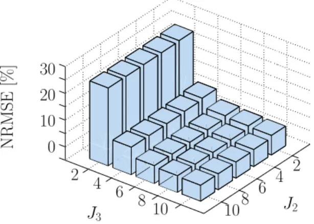
Figure 3 shows the NRMSE of the model as function of the number of orthonormal bases in H2(n1, n2) and H3(n1, n2, n3). Analyzing figure 3, it is possible to observe that the second kernel does not have a great effect in the response of the system while the third kernel has the convergence of the error close to 6 functions. Considering this information the order of the model was considered to be J1 = 2, J2 = 2 and J3 =6 representing the first, second and third order kernels respectively (Step 2).
Figure 3 – Convergence analysis of the Volterra model representing the Duffing oscillator.
J2
J3 0 10
NR
MSE
[%]
20 30
2 4
6 8
2 4 6 8 10 10
Source: Prepared by the author.
After deciding the number of orthonormal functions to be used in the Volterra kernels, the Kautz parameters should be defined (Step 3). An optimization procedure based on sequential quadratic programming (SQP) was used in order to define these parameters (LUENBERGER; YE, 2008). Since the frequencies and damping ratios of the Kautz parameters are generally close to the values describing the linear dynamics of the system, the optimization can search values close to the ones observed in a frequency-domain analysis of the identification data (SHIKI et al., 2014). In this study the Kautz parameters describing the first Volterra kernel (ω1 and ζ1) were fixed in the values of the known natural frequency and damping ratio of the Duffing oscillator. In this way the parameters ω2, ζ2, ω3 and ζ3 were optimized to minimize the NRMSE of the model. The parameters of the SQP optimization are summarized in table 3.
Table 3 – Optimization parameters for the calculation of the Kautz parameters in the Duffing oscillator.
Parameter of the optimization Value
Algorithm SQP
Objective function NRMSE
Number of parameters 4 ([ω2, ζ2, ω3, ζ3])
Maximum number of iterations 1000
Termination tolerance on the variable 10−10 Termination tolerance on the objective function 10−10
Initial guess [26.7 Hz, 1.9 %, 26.7 Hz, 1.9 %]
Lower search bound [21.3 Hz, 0.1 %, 21.3 Hz, 0.1 %]
Upper search bound [32.1 Hz, 5.0 %, 32.1 Hz, 5.0 %]
Source: Prepared by the author.
Table 4 – Information for the identification of the Kautz functions of the Duffing oscillator.
ω1 [Hz] ζ1[%] ω2 [Hz] ζ2[%] ω3 [Hz] ζ3[%] 26.7 1.9 26.9 2.2 26.1 1.3 Source: Prepared by the author.
Figure 4 – Illustration of the first Volterra kernel in the physical basis representing the Duffing oscillator. n1 0.1 0.05 0 -0.05
-0.10 200 400 600 800 100012001400
H1
(a) First Volterra kernelH1.
Frequency [Hz]
10−4
10−6
10−8
10−10
10−12
200 150 100 50 0 PSD [mm
2/Hz]
(b) PSD ofH1
Source: Prepared by the author.
Figure 5 – Illustration of the second Volterra kernel in the physical basis representing the Duffing oscillator.
n1=n2 0
-0.2
-0.4
-0.6
-0.80 100 200 300 400 500 600
diag
(
H2
)
(a) Main diagonal ofH2.
Frequency [Hz]
10−2
10−3
10−4
10−5
10−6
10−7
200 150 100 50 0 PSD [mm
2/Hz]
(b) PSD of the main diagonal ofH2
Source: Prepared by the author.
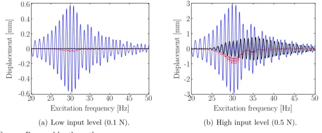
The direct comparison between the response obtained from the numerical integration of the Duffing oscillator and through the Volterra model is illustrated in figure 7 showing a good agreement for a low and high level of displacement. The components of the response of the Volterra model to a chirp excitation in the lowest level of amplitude (0.1 N) and in the highest one (0.5 N) can be observed in figure 8. The increase in y2 and y3 with respect to y1 is evident in this figure. Also it is interesting to see that y2 represents the asymmetry of the displacement in the oscillator due to the quadratic stiffnessk2.
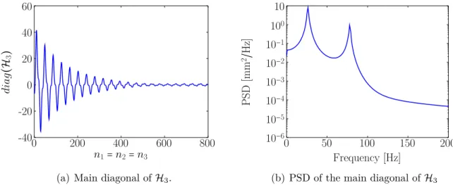
Figure 6 – Illustration of the third Volterra kernel in the physical basis representing the Duffing oscillator.
n1=n2=n3 60
40
20
0
-20
-400 200 400 600 800
diag
(H
3
)
(a) Main diagonal ofH3.
Frequency [Hz] 10
100
10−1
10−2
10−3
10−4
10−5
10−6
200 150 100 50 0 PSD [mm
2/Hz]
(b) PSD of the main diagonal ofH3
Source: Prepared by the author.
Figure 7 – Output of the identified Volterra model. The continuous line --- represents the response of the model and,○ is the response of the Duffing oscillator.
Excitation frequency [Hz] 0.8 0.6 0.4 0.2 0 -0.2 -0.4 -0.6
-0.820 25 30 35 40 45 50
Di
spl
acement
[mm]
(a) Low input level (0.1 N).
Excitation frequency [Hz] 3 2 1 0 -1 -2 -3
-420 25 30 35 40 45 50
Di
spl
acement
[mm]
(b) High input level (0.5 N)
Source: Prepared by the author.
of the system (26.7 Hz).The Fourier series coefficients of the response of the Volterra model as well as its components are depicted in the figures 9 and 10 respectively.
Figure 8 – Components of the response to a chirp input for the Duffing oscillator. The continuous line is the linear component (y1), is the second order nonlinear response (y2) and is the third order nonlinear response (y3).
20 25 30 35 40 45 50
-0.6 -0.4 -0.2 0 0.2 0.4 0.6
Excitation frequency [Hz]
Di
spl
acement
[mm]
(a) Low input level (0.1 N).
20 25 30 35 40 45 50
-3 -2 -1 0 1 2 3
Excitation frequency [Hz]
Di
spl
acement
[mm]
(b) High input level (0.5 N). Source: Prepared by the author.
Figure 9 – Comparison between the Fourier series coefficients of the responses to a sine excitation of the oscillator and the identified model. -○-is the reference signal and -△-is the response of the Volterra model.
Ampl
itude
[mm]
Frequency [Hz] 1.5
1
0.5
0
-0.50 20 40 60 80 100
Source: Prepared by the author.
These separated components can be used to calculate a metric of the degree of non-linearity in the system response modeled by the Volterra model. Figure 11 shows a ratio between the root mean square (RMS) level of the nonlinear components and the root mean square of the total response (RM S(y2+y3)/RM S(y)) as a function of the input level for the case of chirp excitation. Due to the polynomial nature of the stiffness, an increase in the level of nonlinear response can be observed as the displacement of the system is increased.
Figure 10 – Comparison between the Fourier series coefficients of the response components to a sine excitation. -△-is the linear component, -Ԃ-is the second order component and
-○- is the third order component.
Ampl
itude
[mm]
Frequency [Hz] 101
100
10−1
10−2
10−3
10−4
10−5
100 80
60 40 20 0
Source: Prepared by the author.
Figure 11 – Nonlinearity index for the Duffing oscillator.
0.4 0.3 0.2 0.1
Input level [N] 0.5 0
0.1 0.5
R
M
S
(
y2
+
y3
)/
R
M
S
(
y
)
0.4
0.3
0.2
Source: Prepared by the author.
will be used to analyze other nonlinear systems.
2.6
Conclusions
linear and nonlinear responses in a separated way. Although only a single input/single output (SISO) formulation of the model was presented, single input/multiple outputs (SIMO) and multiple inputs/multiple outputs (MIMO) are also perfectly possible but are
not explored in this thesis.
3
Methodologies for the
application in SHM
This chapter presents strategies for the application of Volterra series for structural health monitoring. Section 3.1 shows a brief review of the literature concerning the aspects of SHM involving nonlinearities. Section 3.2 shows a possible option of application for an identified Volterra model as representing the reference state of a structure in a way that the prediction error of the model can be monitored to detect structural variations. Section 3.3 shows the methodology for the parameter quantification using the reference Volterra kernels to estimate physical information of the system. Finally in the section 3.4 some partial conclusions about the methodology are presented.
3.1
Overview of the literature for nonlinear techniques
in SHM
As previously mentioned in chapter 1, a frequently used approach in the damage identification literature is to consider the nonlinear effects caused by the occurrence of damage. Many researchers already used this appealing idea to detect nonlinear damages like cracks, impacts, delamination or rotor-stator rub (NICHOLS; TODD, 2009). Haroon and Adams (2007) shows the characterization of nonlinear behavior in experimental tests on a vehicular suspension system under different simulated damage conditions. Mechani-cal faults in the suspensions are done by the loosening of bolts and cuts in the structure. These damages are identified in the experimental data using nonlinear restoring force surface method and autoregressive models with exogenous input.