www.geosci-model-dev.net/8/1321/2015/ doi:10.5194/gmd-8-1321-2015
© Author(s) 2015. CC Attribution 3.0 License.
Modelling the role of fires in the terrestrial carbon balance by
incorporating SPITFIRE into the global vegetation model
ORCHIDEE – Part 2: Carbon emissions and the role of fires in the
global carbon balance
C. Yue1,2, P. Ciais2, P. Cadule2, K. Thonicke3, and T. T. van Leeuwen4,5
1Laboratoire de Glaciologie et Géophysique de l’Environnement, UJF, CNRS, Saint Martin d’Hères CEDEX, France 2Laboratoire des Sciences du Climatet de l’Environnement, LSCE CEA CNRS UVSQ, 91191 Gif-Sur-Yvette, France 3Potsdam Institute for Climate Impact Research (PIK) e.V., Telegraphenberg A31, 14473 Potsdam, Germany
4SRON Netherlands Institute for Space Research, Sorbonnelaan 2, 3584 CA, Utrecht, the Netherlands 5Institute for Marine and Atmospheric Research Utrecht, Utrecht University, Princetonplein 5,
3584 CC, Utrecht, the Netherlands
Correspondence to:C. Yue ([email protected])
Received: 20 November 2014 – Published in Geosci. Model Dev. Discuss.: 18 December 2014 Revised: 30 March 2015 – Accepted: 14 April 2015 – Published: 6 May 2015
Abstract. Carbon dioxide emissions from wild and anthro-pogenic fires return the carbon absorbed by plants to the at-mosphere, and decrease the sequestration of carbon by land ecosystems. Future climate warming will likely increase the frequency of fire-triggering drought, so that the future terres-trial carbon uptake will depend on how fires respond to al-tered climate variation. In this study, we modelled the role of fires in the global terrestrial carbon balance for 1901–2012, using the ORCHIDEE global vegetation model equipped with the SPITFIRE model. We conducted two simulations with and without the fire module being activated, using a static land cover. The simulated global fire carbon emissions for 1997–2009 are 2.1 Pg C yr−1, which is close to the 2.0 Pg C yr−1 as estimated by GFED3.1. The simulated land car-bon uptake after accounting for emissions for 2003–2012 is 3.1 Pg C yr−1, which is within the uncertainty of the residual carbon sink estimation (2.8±0.8 Pg C yr−1). Fires are found to reduce the terrestrial carbon uptake by 0.32 Pg C yr−1
over 1901–2012, or 20 % of the total carbon sink in a world without fire. The fire-induced land sink reduction (SRfire) is
significantly correlated with climate variability, with larger sink reduction occurring in warm and dry years, in particular during El Niño events. Our results suggest a “fire respira-tion partial compensarespira-tion”. During the 10 lowest SRfireyears
(SRfire=0.17 Pg C yr−1), fires mainly compensate for the
heterotrophic respiration that would occur in a world with-out fire. By contrast, during the 10 highest SRfire fire years
(SRfire=0.49 Pg C yr−1), fire emissions far exceed their
res-piration partial compensation and create a larger reduction in terrestrial carbon uptake. Our findings have important im-plications for the future role of fires in the terrestrial carbon balance, because the capacity of terrestrial ecosystems to se-quester carbon will be diminished by future climate change characterized by increased frequency of droughts and ex-treme El Niño events.
1 Introduction
Vegetation fires contribute significantly to the interannual variability (IAV) of atmospheric CO2concentration.
Defor-estation and peat fires emit carbon that is not offset by rapid vegetation regrowth, and thus contribute to a net increase in atmospheric CO2(Bowman et al., 2009; Langenfelds et al.,
2002; Schimel and Baker, 2002; van der Werf et al., 2009). Besides the direct effect of fires in reducing the capacity of terrestrial ecosystems to sequester carbon, other greenhouse gases (e.g. CH4, N2O), ozone precursors, and aerosols
can also impact climate by changing the land surface prop-erties, such as vegetation structure and albedo (Beck et al., 2011; Jin et al., 2012), as well as the energy partitioning (Liu and Randerson, 2008; Rocha and Shaver, 2011). Changes in temperature and precipitation patterns, in particular drought frequency and severity, also influence fire regimes and their emissions (Balshi et al., 2009; Kloster et al., 2012; Wester-ling et al., 2011), causing complex fire–vegetation–climate interactions.
The estimation of global carbon emissions from fires was pioneered by Seiler and Crutzen (1980), who used avail-able literature data of field experiments to assess important fire parameters like area burned, fuel load and the combus-tion completeness. More recently, large-scale spatially ex-plicit estimation of fire carbon emissions has been aided by satellite-derived burned area and active fire counts (Giglio et al., 2010; Roy et al., 2008; Tansey et al., 2008), as well as vegetation models in which burned area is either prescribed (Randerson et al., 2012; van der Werf et al., 2006, 2010) or simulated with a prognostic fire model (Kloster et al., 2010; Li et al., 2013; Prentice et al., 2011; Thonicke et al., 2010). Several recent estimates have converged to give annual fire carbon emissions of ∼2 Pg C yr−1, as pointed out by Li et
al. (2014). Van der Werf et al. (2006) showed that the IAV of global fire carbon emissions is decoupled from the variation in burned area, mainly due to the disproportionate contribu-tion to global emissions by fires with a large fuel consump-tion (forest fire, deforestaconsump-tion fire and peat fire). Prentice et al. (2011) examined how burned area in tropical and subtrop-ical regions is influenced by the El Niño–Southern Oscilla-tion (ENSO) climate variability, and quantified the contribu-tion of fire emission anomaly to the anomaly of land sink as diagnosed by atmospheric inversions. However, it is only re-cently that Li et al. (2014) have simultaneously constrained the simulated fire carbon emissions and net biome production (NBP, i.e. the land carbon sink) in their absolute terms, em-ploying a modelling approach. These modelled components of the carbon balance have rarely been reported simultane-ously before. Li et al. (2014) also compared the difference in simulated NBP from two simulations with and without fires. However, the specific climatic driving factors for this fire-induced NBP difference have not been investigated. Given the profound perturbation of the climate system by human activities (Cai et al., 2014; Liu et al., 2013; Prudhomme et al., 2013), and with fire activities likely to increase in the future (Flannigan et al., 2009; Kloster et al., 2012), it is therefore important to examine how fires and their contribution to the global carbon balance have responded to historical climate variations. This knowledge will give us insight into the likely impact of fires on the future land carbon balance.
Just as vegetation can be classified into biomes accord-ing to its climatic, morphological and physiological features, so fires occurring under different climate and vegetation pat-terns have distinctive features that allow them to be charac-terized byfire regime. Attributes of different fire regimes
in-clude the frequency, season, size, intensity and extent of fires (Gill and Allan, 2008). Trade-offs may exist between these different aspects of fire; e.g. ecosystems with frequent fires often have a long fire season but can hardly support high-intensity fires because of their low fuel load (Saito et al., 2014). Efforts have been made to further classify fires by ex-amining co-occurring fire characteristics and relating these fire groups (named pyromes) to climatic, human and eco-nomic factors (Archibald et al., 2013; Chuvieco et al., 2008). Archibald et al. (2013) proposed an approach to divide fires into five pyromes, using the most extensive available global fire regime data sets including fire extent, fire season length, fire return interval, fire size and fire intensity. Though related to the biome distribution, pyromes are different from biomes. For example, the “intermediate–cool–small” fire pyrome oc-curs throughout the globe, particular in regions of deforesta-tion and agriculture, whereas the “frequent–intense–large” fire pyrome is associated with tropical grassland-dominated systems. Different fire pyromes are suspected to also have impacts on the amount, seasonality and IAV of fire carbon emissions, and further consequences for the terrestrial car-bon balance.
2 Data and methods
2.1 ORCHIDEE land surface model
ORCHIDEE is a global dynamic vegetation model that sim-ulates the exchange of energy, water and carbon between the atmosphere and the land surface. It is the land surface model of the IPSL-CM5 Earth system model (Dufresne et al., 2013; Krinner et al., 2005). The processes and equations of the SPITFIRE fire model (Thonicke et al., 2010) were imple-mented in ORCHIDEE, with some modifications being de-scribed in Yue et al. (2014). There, the model was evaluated against different satellite observations for simulated burned areas and fire regimes.
The SPITFIRE module simulates burned area and fire con-sequences (e.g. emissions, plant mortality) in a mostly mech-anistic way. The central underlying engine is the Rothermel fire spread model (Rothermel, 1972; Pyne et al., 1996; Wil-son, 1982), which links fire spread rate to fuel state, weather conditions and fire physics. Weather and fuel moisture con-ditions determine the time that a fire persists, which, com-bined with fire spread rate, yields an estimate of mean fire size. Ignition sources are scaled into fire numbers depend-ing on weather conditions, with sources from both lightndepend-ing and human activities being included. The daily burned area is thus derived as the product of fire number and mean fire size. Anthropogenic ignitions are estimated as a function of pop-ulation density with the maximum ignition being obtained at ca. 16 ind km−2 (Venevsky et al., 2002; Thonicke et al., 2010). Anthropogenic ignitions are implicitly suppressed by humans within the ignition equation, while lightning igni-tions are not suppressed.
Fire carbon emissions follow a classical paradigm (Seiler and Crutzen, 1980) as the product of daily burned area, fuel load, and combustion completeness. Dead litter on the ground and live biomass from grasses and trees are available for burning. For live grass biomass and dead litter, combus-tion completeness is calculated as a funccombus-tion of fuel moisture state following the approach of Peterson and Ryan (1986). Tree crown live biomass consumption is simulated to depend on fire intensity and fire scorching height. Two factors are considered concerning fire-caused tree mortality: damage to tree crown because of crown scorching; and cambial damage linked with fire persistence time and tree bark resistance to fire. We refer the reader to Yue et al. (2014) and Thonicke et al. (2010) for a more detailed description of the fire module. The simulation of combustion completeness (CC) for sur-face dead fuel was modified compared to the original scheme as presented by Thonicke et al. (2010). In SPITFIRE, the calculation of surface fuel CC follows Peterson and Ryan (1986), which allows CC to increase with decreasing fuel wetness and level out when the fuel wetness drops below some threshold (see Fig. 1 in Yue et al., 2014). During the model testing, it was found that simulated CCs were much higher than the recently compiled field observations for
dif-ferent biomes (van Leeuwen et al., 2014). We thus adjusted the maximum CC for fuel classes of 100 (with original max-imum CC as 1.0) and 1000 h (with original maxmax-imum CC as 0.8) to mean values provided by an earlier version of van Leeuwen et al. (2014) (R. G. Detmers, personal communica-tion) which was available when preparing the current study. The categorization of fuels in terms of magnitude of hours describes the order of magnitude of time required to lose (or gain) 63 % of the fuel moisture difference with the equi-librium moisture state under defined atmospheric conditions (Thonicke et al., 2010). The mean observational values were adopted as the maximum values in the model equations, be-cause the simulated burned area is dominated by low fuel wetness, so that the simulated CC value is close to its maxi-mum. However, we kept the original CC simulation scheme in the original SPITFIRE model for the convenience of fu-ture elaboration. According to the earlier-version data set of van Leeuwen et al. (2014), the biome-dependent maximum CC is 0.49 for tropical broadleaf evergreen and seasonal dry forests, 0.45 for temperate forests, 0.41 for boreal forests, and 0.85 for grasslands.
2.2 Model productivity calibration
As shown by Yue et al. (2014), the mean annual burned area on non-crop lands for 2001–2006 was simulated to be 346 Mha yr−1 by ORCHIDEE. This falls within the range 287–384 Mha yr−1 from three global satellite-derived data sets (GLOBCARBON, L3JRC and GFED3.1), and is close to the 344 Mha yr−1obtained in GFED3.1 when agricultural
fires are excluded. The simulated global burned area on a decadal timescale during the twentieth century agrees mod-erately well with the historical reconstruction by Mouillot and Field (2005), corrected for regional mean bias using GFED3.1 for 1997–2000. However, one ORCHIDEE model shortcoming is that the terrestrial productivity is overesti-mated (as also revealed by Piao et al., 2013), possibly due to the absence of nutrient limitation, which leads to overesti-mated fire carbon emissions.
The simulated global gross primary productivity (GPP) by ORCHIDEE (version 1.9.6) as driven by CRUNCEP cli-mate forcing data is 205 Pg C yr−1 for 1982–2010. This is much higher than the estimated 119±6 Pg C yr−1 by
Jung et al. (2011), which was derived by interpolating eddy-covariance measurements over the globe using climate, remote-sensing fAPAR and a multiple tree regression ensem-ble algorithm (hereafter referred to as MTE-GPP). In order to correct for the positive bias of GPP, we use a simple ap-proach to adjust the optimal carboxylation rates (Vcmax, in
unit of µmol m−2s−1, see Eqs. (A2)–(A6) in Krinner et al., 2005) to match the simulated total GPP with the MTE-GPP reported for different biomes.
agricultural land. The spatial extent of each biome was deter-mined as the area where a corresponding ORCHIDEE PFT occupies more than 90 % of a grid cell in the 0.5◦MTE-GPP
data set. A ratio of simulated GPP to MTE-GPP was deter-mined for each biome, and this ratio was used to adjust car-boxylation rates (with the maximum potential rate of RuBP regeneration Vjmax being set to double that of Vcmax). The
original and calibrated carboxylation rates together with the biome-specific GPP ratios are given in Table S1 in the Sup-plement. We emphasize that the approach employed here is an empirical and simple adjustment to calibrate ORCHIDEE productivity, but does not necessarily result in optimized car-boxylation rates that agree with, for example, leaf-scale mea-surements (e.g. see discussion by Rogers, 2014).
2.3 Simulations and input data sets
To evaluate the role of fires in the global terrestrial carbon balance, two parallel simulations were conducted: fireON and fireOFF, with SPITFIRE being switched on or off, respectively. In both simulations, the dynamic vegetation module of ORCHIDEE was de-activated, and a current-day vegetation distribution map (converted into the 13-PFT map in ORCHIDEE based on the IGBP 1 km veg-etation map, http://webmap.ornl.gov/wcsdown/dataset.jsp? ds_id=930) was used as the static land cover. Here, fire– vegetation–climate feedback was not included because the relative fractions of different PFTs remain the same over the simulation period. It means not only that fires associated with land-cover change (deforestation fires) are not included, but also that wildfires are not affected by changing PFTs.
Agricultural fires are not simulated in the model for two reasons. First, the timing of agricultural burning is strongly constrained by the sowing and harvest dates (Magi et al., 2012). An enhanced crop phenology module is under devel-opment for ORCHIDEE and this will allow precise agricul-tural fire seasons to be included in the future. Second, agri-cultural fires are normally under strict human control and the spread and size of fires are limited by field size; they are thus very different from wildfires and warrant a special modelling approach. Carbon emissions from tropical and boreal peat fires are not explicitly simulated, although the model does simulate some burned fractions in tropical regions where de-forestation fires dominate, because the model could capture the “climate window” when the climate is relatively dry and deforestation fires are possible. Thus, even though the model does not explicitly simulate deforestation fires using a land-cover-change approach, it does capture some fire activities in the region dominated by deforestation fires, and simu-lates them like natural wildfires. Figure S1 in the Supplement compares simulated and GFED3.1 emissions for the tropi-cal region of 20◦S–20◦N for different types of fire averaged over 1997–2009. The simulated fire emissions were parti-tioned into forest and grassland fires, and the GFED3.1 emis-sions were partitioned into “deforestation+forest”,
“wood-land+savanna”, and “agriculture+peat”. The model could capture part of forest and deforestation fire emissions in this region (simulated 0.28 Pg C yr−1against GFED3.1 0.44 Pg
C yr−1, of which deforestation fires account for 0.33 Pg C yr−1 and naturally occurring forest fires 0.11 Pg C yr−1), because simulated total forest fire emissions in this region are larger than those from natural forest fires as given by GFED3.1 data. The simulated emissions are slightly lower than GFED3.1 data, even when emissions from agriculture and peat fires are excluded (simulated 1.38 Pg C yr−1 for forest+grassland against GFED3.1 1.50 Pg C yr−1for
de-forestation+forest +woodland+savanna, and 1.63 Pg C
yr−1 when agriculture and peat are further included). This shows that the model has limited capability in capturing fire emissions in tropical regions.
Both fireON and fireOFF simulations followed the same protocol, which comprised three steps. For both simulations, the model was first run for 200 years (including a 3000-year soil-only spin-up to speed up the equilibrium of slow and passive soil carbon pools) starting from bare ground without fire, with atmospheric CO2being fixed at the pre-industrial
level (285 ppm) and climate data of 1901–1930 being cycled. For the fireON simulation, after this first spin-up, the model was run for a second spin-up of 150 years with the fire model being switched on, to allow carbon stocks to reach an equi-librium state under pre-industrial fire disturbance. For this second spin-up with fires, atmospheric CO2 was set at
pre-industrial level and climate data of 1901–1930 were cycled. We verify that during last 50 years of this second spin-up, the mineral soil carbon stock (i.e. the sum of active, slow and passive soil carbon pools in the model) varies within 0.1 % and no significant trend exists for simulated global total car-bon balance. This simulation was followed by a third tran-sient simulation for 1850–2012, with variable climate, atmo-spheric CO2and population density data.
For the fireON simulation, after the second spin-up, there is a global carbon sink of 0.19 Pg C yr−1 over the last
50 years prior to the transient simulation due to the not-fully complete equilibrium of slow soil carbon pools. We verified that this sink has a negligible trend (annual trend of 0.003 Pg C yr−1). For the fireOFF simulation, the residual sink before the transient simulation is 0.17 Pg C yr−1(with a negligible annual trend of−0.001 Pg C yr−1). Because the ORCHIDEE version used here is computationally expensive, we did not run the model until a complete carbon saturation state. The simulated annual global total net biome production (NBP) during 1901–2012 was bias-corrected for this incom-plete spin-up by subtracting the remaining positive NBP over the last 50 years of the second spin-up. No spatial corrections were made.
2.4 Land–atmosphere carbon flux conventions We define NEP, the net ecosystem production, as
NEP=NPP−RH−CH, (1)
where NPP is net primary production, RH is the het-erotrophic respiration, and CH is the harvested crop yield. We assume that crop harvest is released into the atmosphere within the year of harvest. Next, we define NBP, the net biome production, as
NBP=NEP−FE, (2)
where FE is fire carbon emission. In case of fireOFF sim-ulation, fire carbon emissions would be zero. If we do not include other components of the carbon balance term (e.g. herbivore consumption, biogenic volatile organic compound emissions, lateral carbon transfer by rivers and erosion), NBP is here considered as a land carbon sink. We expect that fires will reduce this carbon sink, and define the fire-induced sink reduction as
SRfire=NBPOFF−NBPON, (3)
where NBPOFFis NBP by fireOFF simulation and NBPONis
NBP by fireON simulation. We further define the term “sink efficiency (SE)” as NBP divided by NPP, which describes the fraction of NPP used to sequester carbon from the atmo-sphere.
2.5 Evaluation data sets and other data sets
The GFED3.1 fire carbon emissions from the CASA bio-sphere model forced by GFED3.1 burned area data were used to evaluate simulated fire carbon emissions (van der Werf et al., 2010). Much work has been done to calibrate the CASA model against observations, e.g. in terms of produc-tivity and NPP allocation (van der Werf et al., 2006, 2010). Carbon emissions from six different fire types are identified
in GFED3.1 data, namely forest fire, grassland fire, wood-land fire, agricultural fire, deforestation and peatwood-land fire. For convenience of description, emission sources of the for-mer three types of fire are tentatively referred to as natural sources (that ORCHIDEE–SPITFIRE simulates explicitly), and those of the latter three types as anthropogenic sources (that ORCHIDEE does not explicitly include, although it is able to capture part of the deforestation fire emissions as ex-plained in Sect. 2.3). Note that the grouping of different emis-sion sources in GFED3.1 data does not necessarily reflect the exact nature of different fire types. For example, peat fires in tropics are mainly due to intentional drainage followed by burning to remove a (logged) forest (thus anthropogenic, e.g. Marlier et al., 2015), while in northern high-latitude re-gions, peatland fires might be due to drought (thus natural, e.g. Turetsky et al., 2011).
Not all anthropogenic carbon emissions (mainly from fos-sil fuel consumption, cement production and deforestation) into the atmosphere remain there, and some of them are absorbed by the terrestrial ecosystem (land sink) and the ocean (ocean sink). The so-called residual carbon sink in land ecosystems can be obtained by subtracting the annual CO2
accumulation in the atmosphere and the ocean sink from the total anthropogenic carbon emissions (Le Quéré et al., 2013). This residual sink was used here to be compared with a sim-ulated carbon sink.
The fire variability at global and regional scales is known to relate to the ENSO mode of climate variability (Kitzberger et al., 2001; Prentice et al., 2011; van der Werf et al., 2004), mainly affecting the tropics but with global teleconnec-tions (Kiladis and Diaz, 1989). The Southern Oscillation In-dex (SOI, http://www.bom.gov.au/climate/current//soihtm1. shtml) is an indicator of the development and intensity of El Niño or La Niña events in the Pacific Ocean (negative values of the SOI below−8 often indicate El Niño episodes and the
reverse La Niña episodes). SOI was used here to investigate the fire-induced sink reduction in relation to this large-scale climate oscillation.
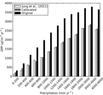
Figure 1. Annual GPP as a function of annual precipitation ac-cording to Jung et al. (2011) (dashed bar); model simulation before (black bar) and after calibration (grey bar).
3 Results and discussion
3.1 Calibrated productivity and simulated burned area The calibration of carboxylation rates significantly improved the model–observation agreement in terms of the distribution of GPP as a function of annual precipitation (Fig. 1). The calibrated model is also able to capture the productivity de-crease when annual precipitation exceeds 3000 mm (Fig. 1). The simulated global GPP for 1982–2010 is 125 Pg C yr−1, close to the 119±6 Pg C yr−1given by Jung et al. (2011).
The simulated global NPP for 2000–2009 is 61 Pg C yr−1, close to the 54 Pg C yr−1estimated by Zhao and Running (2010) using MODIS satellite data and light-use efficiency conversion factors.
The simulated global burned area for 2001–2006 is 239 Mha yr−1, lower than the original 346 Mha yr−1
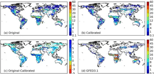
be-fore calibration (Yue et al., 2014). This reduction in sim-ulated burned area mainly occurs in the regions with high fire frequency where GPP was decreased by the calibra-tion (Fig. 2). After the GPP calibracalibra-tion, the burned frac-tion of grassland and savanna ecosystems in Africa, Aus-tralia and South America became underestimated compared to GFED3.1 (Fig. 2b and d). The reduction in simulated burned fraction is related to the reduced amount of dead fuel on the surface (Fig. S3) in response to the lower GPP – the latter reduces fire spread rates and fire sizes.
3.2 Temporal and spatial patterns of global fire carbon emissions
3.2.1 Comparison of simulated carbon emissions with GFED3.1 at the global scale
The simulated mean annual global fire carbon emissions for 1997–2009 are 2.1 Pg C yr−1, close to the estimate of 2.0 Pg C yr−1 by GFED3.1 data, where emissions from both nat-ural and anthropogenic sources are included (Fig. 3), and higher than the 1.5 Pg C yr−1when peat, deforestation and
agricultural fires are excluded from GFED3.1. The model also simulates lower IAV of emissions than GFED3.1, giving a coefficient of variation of 0.05, compared to 0.18 for the GFED3.1 data (0.15 when only natural sources are included in GFED3.1).
The interannual variability of fire carbon emissions is known to be partially decoupled from that of burned area (van der Werf et al., 2006), mainly because emission vari-ability is driven by forest fires with higher fuel consumption, whereas burned area variability is driven by savanna fires with relatively large burned fraction but low fuel consump-tion. At the global scale, the IAV of fire carbon emissions is simulated to be closely related to that of burned area (Fig. S4, giving a correlation coefficient of 0.88 over 1997–2009 – all data detrended). In contrast, the correlation coefficient be-tween GFED3.1 natural source emissions and burned area is 0.52 over the same period (0.04 when emissions from both natural and anthropogenic sources are included), i.e. smaller than ORCHIDEE–SPITFIRE. Thus the IAV of carbon emis-sions is more strongly coupled to that of burned area in OR-CHIDEE than in GFED3.1, because emissions are dominated by burning of litter (from grassland, savanna and forest) and are less driven by forest fires that involve a large amount of live biomass burning.
3.2.2 Comparison of simulated carbon emissions with GFED3.1 for different regions
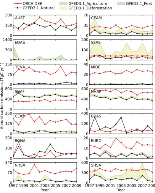
Annual fire carbon emissions simulated by ORCHIDEE– SPITFIRE are compared with GFED3.1 data for 1997–2009 for different regions in Fig. 4 (see figure caption for expan-sion of GFED region abbreviations and Fig. S5 for region distribution). The three regions with the most frequent fires, Northern Hemisphere Africa (NHAF), Southern Hemisphere Africa (SHAF) and Australia (AUST), have total fire emis-sions of 1.17 Pg C yr−1and contribute 59 % of the global
to-tal emissions in GFED3.1. In ORCHIDEE, annual emissions are 1.18 Pg C yr−1for these three regions, an overestimation in NHAF being partly compensated for by underestimation in SHAF.
Figure 2.Simulated mean annual burned fraction (%) for 1997–2009 for(a)original and(b)calibrated model productivity. The change in burned fraction (original–calibrated) is shown in panel(c), and the burned fraction by GFED3.1 data is shown in panel(d).
Table 1.Comparison of simulated and GFED3.1 fire carbon emissions, burned area and total fuel consumption (TFC, including consumption of surface dead litter or organic soil, and live biomass) for different regions averaged over 1997–2009. The locations of the GFED regions are mapped in Fig. S5, the abbreviations expanded in the caption to Fig. 4. The last three columns provide a qualitative indication of the error in simulated carbon emissions and its attribution to those of burned area and TFC. To obtain the qualitative error information, the ratio of the simulated value to GFED3.1 is compared to the coefficient of variation (CV) of the corresponding GFED3.1 value as follows:
=, no error, if the ratio is within (1−CV, 1+CV); +, overestimated, if the ratio falls in (1+CV, 3); ++, moderately overestimated, if the ratio falls in (3,10); + + +, highly overestimated, if the ratio is bigger than 10; -, underestimated, if the ratio falls in (0.3, 1−CV); and - -, moderately underestimated, if the ratio falls in (0.1, 0.3).
The CV for annual emissions and burned area by GFED3.1 data was calculated using the annual time series. Total fuel consumption data for GFED3.1 were obtained from Table 4 of van der Werf et al. (2010) and an arbitrary CV of 0.3 was adopted.
Region
Emissions Burned area Total fuel Emission BA error TFC error (Tg C yr−1) (Mha yr−1) consumption error
(g C m−2of BA)
GFED3.1 ORC GFED3.1 ORC GFED3.1 ORC
BONA 54 45 2.1 3.3 2662 1385 = =
-TENA 9 96 1.5 18.5 627 514 + + + + + + =
CEAM 20 29 1.4 4.1 1489 714 = +
-NHSA 22 79 2.1 5.8 1007 1351 ++ + +
SHSA 272 369 20 35.7 1311 1035 = + =
EURO 4 13 0.7 1.5 667 874 ++ + +
MIDE 2 24 0.9 8.8 198 278 + + + + + + +
NHAF 480 680 129 58.7 377 1159 + - ++
SHAF 556 331 125 34.1 448 969 - - - +
BOAS 128 61 6.6 3.9 1979 1589 - - =
SEAS 103 40 14 4.1 253 969 - - ++
CEAS 35 161 7 41.4 1459 388 ++ ++
-EQAS 181 2 1.8 0.1 9500 1559 - - - -
-AUST 133 174 52 15.6 259 1118 = - ++
Global∗ 1999 2104 364 236 549 891 = - +
Figure 3.Annual global fire carbon emissions for 1997–2009 sim-ulated by ORCHIDEE (blue), and from the GFED3.1 data. Car-bon emissions from natural sources (forest fire, grassland fire, and woodland fire) are shown as the black solid line. Carbon emissions from agricultural fire, deforestation fire and peat fire (which are not explicitly simulated in ORCHIDEE) are shown as shaded areas stacked on top of GFED3.1 natural source fire carbon emissions.
ORCHIDEE–SPITFIRE simulates much higher emissions (294 Tg C yr−1; 14 % of the global total), possibly because
forest fire control measures (Fernandes et al., 2013; Keeley et al., 1999) and forest management in temperate countries (Fang et al., 2001; Luyssaert et al., 2010) are not modelled; this leads to a higher burned area and/or higher fuel load in the model. The overestimation of emissions in these three re-gions is partly driven by the overestimation of burned area (annual burned area of 70.2 Mha yr−1 in the model versus 10.1 Mha yr−1in GFED3.1 in Table 1).
The three regions where the model underestimates carbon emissions are boreal Asia (BOAS), Southeast Asia (SEAS) and equatorial Asia (EQAS), with simulated emissions of 103 Tg C yr−1 (4.9 % of the global total), compared with 412 Tg C yr−1in GFED3.1 (21 % of the global total). The low bias of emissions in BOAS and SEAS is explained by the underestimation of burned area (Table 1), whereas for EQAS, underestimates in both burned area and fuel consumption by the model are found (Table 1) (in particular, peat burning that dominates emissions in 1997–1998 in SEAS is lacking in the model; see van der Werf et al., 2008). This points to the need to explicitly include deforestation and peat fires, which are associated with a high amount of fuel consumption (van der Werf et al., 2010).
3.2.3 Fire fuel consumption and latitudinal pattern of emissions
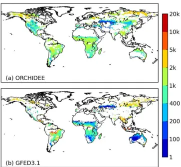
Simulated fuel consumption (g C per m2 of area burned) in fire is compared to GFED3.1 data in Fig. 5. Both ORCHIDEE–SPITFIRE and GFED3.1 show a large amount
of fuel consumption in boreal regions, but fuel consump-tion in the Russian boreal forest is smaller in the model than GFED3.1 (simulated 400–2000 g C m−2compared to 2000–
5000 g C m−2in GFED3.1). The model also fails to capture the high fire fuel consumption (5–20 kg C m−2) at the south-ern edge of the Amazonian rainforest and in Southeast Asia, which are associated with deforestation fires or peat fires (see also Figs. 6 and 13 in van der Werf et al., 2010). The fire fuel consumptions for savannas and woodland savannas in Africa and Australia are higher in the model than GFED3.1, with fuel consumption in northern Africa of 1000–2000 g C m−2 against 200–1000 g C m−2 by GFED3.1. In southern Africa, ORCHIDEE produces fuel consumption of 1000– 2000 g C m−2against only 400–1000 g C m−2in GFED3.1. The simulated higher fuel consumption in tropical savannas and woodland savannas might be due to a combination of overestimated fuel load and combustion completeness, which is discussed in more detail in Sect. 3.2.4. Furthermore, we acknowledge the fact that ORCHIDEE can have grass and tree PFTs coexisting on the same grid point, but does not de-scribe woody savannas or miombo forests where grass and trees compete locally for water, light and nutrients and could have lower fuel consumptions due to the presence of fire-resistant tree species (Hoffmann et al., 2012).
Figure 6 shows carbon emissions per grid cell area (g C per m2 of grid cell) calculated as the product of fire fuel consumption (Fig. 5) and burned fraction (Fig. 2). Because underestimated burned fractions in African and Australian savannas and woodland savannas compensate for overes-timated fuel consumption, fire carbon emissions per grid cell for these regions are of similar magnitude to those in GFED3.1. Emissions per grid cell area in southern African woodland savanna are even underestimated by ORCHIDEE (10–50 g C m−2yr−1)compared with GFED3.1 (50–200 g C m−2yr−1), due to the great underestimation in burned area.
By looking at the latitudinal distribution of burned area and emission, the systematic error in ORCHIDEE’s esti-mated emissions can be clearly related to that in burned areas (Fig. 7). The underestimation of burned area in tropical and subtropical regions (30◦S–15◦N) (Fig. 2) is compensated for by the overestimated fire fuel consumption. In southern trop-ical regions (30◦S–0◦), carbon emissions are still underesti-mated (by 270 Tg C yr−1)despite this compensation effect, whereas in northern tropical regions (0–15◦N), the compen-sation leads to overestimated emissions (by 190 Tg C yr−1)
compared with GFED3.1.
Figure 4.Annual fire carbon emissions simulated by ORCHIDEE and from the GFED3.1 data for 1997–2009 for the 14 different GFED regions. The 14 GFED regions are BONA: boreal North America; TENA: temperate North America; CEAM: Central America; NHSA: Northern Hemisphere South America; SHSA: Southern Hemisphere South America; EURO: Europe; MIDE: Middle East; NHAF: Northern Hemisphere Africa; SHAF: Southern Hemisphere Africa; BOAS: boreal Asia; CEAS: central Asia; SEAS: Southeast Asia; EQAS: equatorial Asia; and AUST: Australia and New Zealand. Refer to Fig. S5 for their distributions.
the GFED3.1 data (where NPP is from the CASA biosphere model, with all GFED3.1 data in Table S2 obtained from Ta-ble 4 in van der Werf et al., 2010). For all regions (except NHAF and AUST) where emissions are overestimated by the model (TENA, CEAM, NHSA, SHSA, EURO, MIDE, CEAS), there is a coincident overestimation in burned area, which sometimes overrides the underestimated fuel con-sumption in regions such as CEAM. Regions where emis-sions are underestimated also show underestimated burned area (with the exception of BOAS), some of them also hav-ing underestimated fuel consumption (EQAS).
The simulated NPP regional averages are in general agree-ment with those from the CASA model reported by van der
Figure 5. Fuel consumption (g C per m2 of area burned) aver-aged over 1997–2009 by (a)ORCHIDEE simulation and (b)the GFED3.1 data.
biomass combined in NHAF, SHAF and AUST contributes to the higher fuel consumptions in these regions, given the fact that simulated NPP is rather similar to GFED3.1 over these regions (except for NHAF, where the simulated NPP is 40 % higher than GFED3.1 and combustion completeness is 2.6 times higher). A recent comparison among different fuel load products by Pettinari et al. (2015) also indicates that our simulated fuel loads in savannas and shrublands are higher than their fuel-model-based data, consistent with the higher NPP in Africa and Australia (Table S2). At the same time, one should also keep in mind that GFED3.1 is not com-pletely an observation data set, but is another model calcula-tion of fire emissions. Given the availability of the compre-hensive fuel combustion field data recently compiled by van Leeuwen et al. (2014), more careful calibration and valida-tion of the simulated combusvalida-tion completeness for different fuel types could be performed in the future.
Finally, the combustion completeness (CC) values used for the 100 and 1000 h dead fuel for temperate forests, bo-real forests and grasslands are slightly different from those reported by van Leeuwen et al. (2014). The mean CC val-ues for the latter three biomes as updated in van Leeuwen et al. (2014) are 0.69±0.13, 0.47±0.16, and 0.81±0.16, re-spectively. The CC values for boreal forests and grasslands used here are within the uncertainty range by van Leeuwen et al. (2014). The CC value for temperate forests is higher than van Leeuwen et al. (2014). We developed a simple ap-proach to adjust the simulated fire carbon emissions for these three biomes by multiplying the simulated emissions by the ratio of our CC values to those of van Leeuwen et al. (2014), and found that the global total fire carbon emissions remain
Figure 6.Mean annual carbon emissions (g C m−2)for 1997–2009 by(a)ORCHIDEE simulation and(b)the GFED3.1 data, based on the whole grid cell area that included both burned and unburned parts.
almost the same (2.1 Pg C yr−1versus 2.08 Pg C yr−1 be-fore and after adjustment for 1997–2009). This is because the smaller CC values used for temperate and boreal forests are compensated for by the larger CC value of grasslands used in the model.
3.3 The role of fires in the terrestrial carbon balance 3.3.1 The simulated carbon balance for the last decade
(1993–2012)
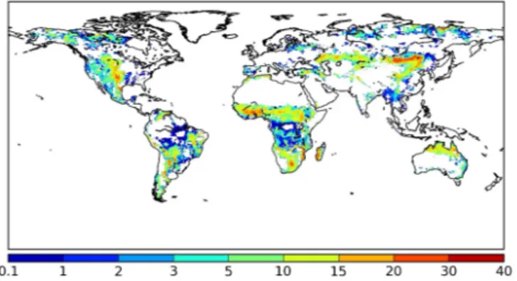
Figure 8 shows the percentage of NPP emitted by fire over the last decade (2003–2012). Regions with frequent burn-ing show a higher fraction of NPP beburn-ing returned to the at-mosphere by fire. Yet, heterotrophic respiration remains the dominant pathway for returning NPP to the atmosphere, ac-counting for 85.7 % of the global NPP (91.1 % when agri-cultural harvest is included, the CH term in Eq. 1). Fire car-bon emissions account for 3.4 % of NPP, with the remaining 5.2 % of NPP being accumulated in the biosphere as a carbon sink (NBP) (as mentioned in Sect. 2.3, the remaining positive NBP of 0.19 Pg C yr−1is subtracted here, taking account of
0.3 % of NPP). The simulated global NPP for 2003–2012 is 60 Pg C yr−1 in the fireON simulation, with 2.1 Pg C yr−1
Figure 7.The latitudinal distribution of(a)burned area and(b)fire carbon emissions as simulated by ORCHIDEE (grey solid line) and by the GFED3.1 data (black dashed line).
Figure 8.The fire carbon emissions as percentage (%) of net pri-mary production (NPP) for 2003–2012.
slightly lower than the 2003–2012 average for grassland fires such as in central and eastern Asia (Fig. S6).
3.3.2 Fire-induced terrestrial carbon sink reduction for 1901–2012
The different components of global carbon fluxes for the fireON and fireOFF simulations are shown in Fig. 9. Net pri-mary production (NPP) for fireON and fireOFF is very sim-ilar (NPP is 6 Tg C yr−1higher in fireOFF for 1901–2012) (Fig. 9a). This greater NPP in the fireOFF simulation com-pared with fireON might be underestimated, because land-cover change or vegetation dynamics were ignored in the simulations (for example, bigger forest coverage would have occurred in the fireOFF simulation if vegetation dynamics were modelled).
The carbon sink in fireOFF is greater than that in fireON (Fig. 9c). This is because fire emissions (1.91 Pg C yr−1 for 1901–2012) are greater than the heterotrophic respira-tion excess in fireOFF (Fig. 9b, by 1.62 Pg C yr−1averaged over 1901–2012). The fire-induced sink reduction (SRfire)
Figure 9.Different components of global carbon fluxes for fireON and fireOFF simulations. The carbon fluxes are(a)NPP;(b) het-erotrophic respiration (RH);(c)NBP and the residual land sink as reported by Le Quéré et al. (2013); and(d)the NBP reduction by fires (SRfire=NBPOFF−NBPON, in grey, left vertical axis) and
fire carbon emissions (black, right vertical axis).
included in the model, because carbon released from these fires is more likely an irreversible net carbon source; i.e. it will not be re-absorbed by post-fire plant recovery on a cen-tennial timescale.
The small fire-induced carbon sink reduction obtained in this study, when only natural wildfires are modelled and with static vegetation cover, implies that if carbon stocks in the fuel (dominated by litter or organic soil except in cases of peat and deforestation fires) were not consumed in fires, they would have been decomposed and have contributed to the heterotrophic respiration. This suggests a fire respiration par-tial compensation in the model; i.e. fire carbon emissions are somewhat analogous to heterotrophic respiration, and when fires are extreme their emissions would far exceed their role of respiration compensation, causing a larger net reduction in carbon sink compared to a world without fire. The sink reduction variability is closely correlated with fire emission anomalies during 1901–2012 (with a correlation coefficient of 0.71, Fig. 9d). Fire carbon emissions show an acceleration of 1.8 Tg C yr−2prior to 1970, and a trend of 6 Tg C yr−2 af-ter 1970, with both trends being significant at the 0.05 level.
Our simulated cumulative land carbon sink (NBP) for 1959–2012 is 109.6 Pg C (with 80.8 Pg C stored in live biomass and 28.8 Pg C in litter and soil), which is close to the cumulative residual sink of 105.9 Pg C (Le Quéré et al., 2013). The cumulative land sink in fireOFF is 127.2 Pg C, suggesting a cumulative sink reduction of 17.6 Pg C by fire since 1959. The correlation coefficient between detrended time series of NBP by the fireON simulation and the residual sink is 0.59, indicating that the model is moderately success-ful at capturing the IAV of the carbon sink by the terrestrial ecosystem.
Prentice et al. (2011) pointed out that fire emissions ac-count for one-third and one-fifth of the IAV of the 1997– 2005 global carbon balance as indicated by atmospheric in-versions, when emissions were from the GFED3.1 data and simulated by the LPX vegetation model, respectively. In our study, fire carbon emissions explained 20 % of the IAV of simulated NBP (which is the R2of the linear regression of detrended annual NBP against simulated carbon emission), congruent with their results.
3.3.3 Fire-induced carbon sink reduction for extreme high and low fire years
We selected 10 “high fire years” as the 10 years with the highest global fire-induced sink reduction (SRfire) during
1901–2012 (Fig. 9d), and 10 “low fire years” as the years with the 10 lowest global SRfireduring the same period. The
average SRfirefor the high fire years is 0.49 Pg C yr−1(23 %
of the fireOFF NBP), compared with an average SRfire of
0.17 Pg C yr−1(7 % of the fireOFF NBP) for the 10 low fire years.
The Pearson correlation coefficient (r) between the SRfire
time series and other model variable or climatic drivers
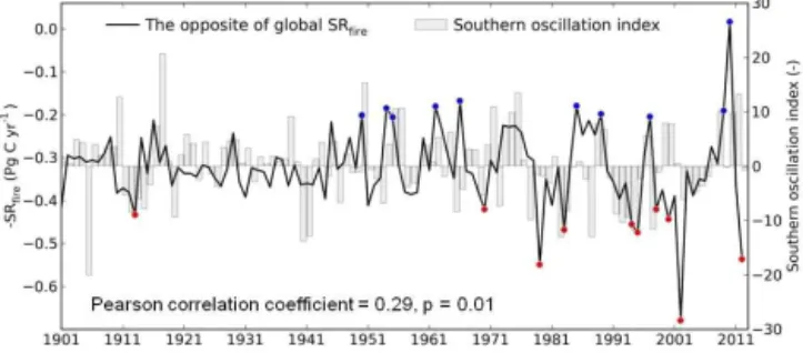
(tem-Figure 10. The fire-induced sink reduction (left vertical axis, −SRfire) and its correlation with the Southern Oscillation Index
(SOI, right vertical axis), which is an indicator of the El Niño South-ern Oscillation (ENSO) climate oscillation. The red dots indicate the 10 highest SRfireyears and the blue dots indicate the 10 lowest
SRfireyears. Note that the left vertical axis shows the opposite of SRfire.
perature, precipitation) was used to investigate the driving factors for fire-induced sink reduction. The SRfire variation
was found to be best explained by fire numbers (r=0.65, p <0.05) within the model, since fire numbers are also driv-ing the variation of burned area (r=0.81,p <0.05). SRfire
is also positively correlated with land surface temperature (r=0.16,p=0.08), and negatively correlated with precip-itation (r= −0.23, p <0.05), although the correlation is fairly weak.
The opposite of SRfire is positively correlated with
the Southern Oscillation Index (SOI) (r=0.29, p <0.05, Fig. 10), suggesting that global fire-induced sink reduction is significantly related to the change in the tropical Pacific sea-surface temperature gradient, because of its strong influence over global rainfall (Ropelewski and Halpert, 1987, 1996). The El Niño state (i.e. low SOI value) of climate oscillation generally coincides with larger sink reduction by fires (i.e. larger SRfire), and La Niña with smaller reduction. Indeed, 7
out of the 10 high fire years occur during El Niño episodes, and 6 out of the 10 low fire years occur during La Niña episodes (the diagnosis of El Niño and La Niña episodes is given by the Bureau of Meteorology of the Australian gov-ernment, http://www.bom.gov.au/climate/enso/lnlist/). SRfire
is more strongly related to SOI in tropical regions than at the global scale thanks to the more direct impacts of ENSO events (for 30◦S–30◦N, the relationship between −SRfire
and SOI yields r=0.33 with p <0.05). This region con-tributes 82 and 72 % of global total emissions and carbon sink, respectively.
der Werf et al., 2004, 2010) are not included. The underesti-mated IAV in fire carbon emissions by the model might lead to underestimated temporal variability in SRfire; thus the
ac-tual correlation between fire-induced sink reduction and SOI over the historical period might be underestimated.
Despite the fact that systematic bias exists for simulated burned area, as global total fire carbon emissions are con-strained with the GFED3.1 estimate, the estimated long-term average SRfireremains reliable. To verify this, we forced the
model with observed GFED3.1 burned area data for 1997– 2009 on a monthly time step and used the regional specific combustion completeness values as reported in van der Werf et al. (2010) (Table 4 in van der Werf et al., 2010, for the 14 regions). The forced simulation yields annual global fire car-bon emissions of 1.8 Pg C yr−1for 1997–2009 and an SR
fire
of 0.39 Pg C yr−1, close to the fire emissions of 2.1 Pg C
yr−1and SR
fireof 0.36 Pg C yr−1as given by the prognostic
simulation.
The suggested “respiration partial compensation” by fires (i.e. larger sink reduction with more extreme fires), and the strong relevance of SRfire to climatic variations (i.e., larger
sink reduction during warm and dry El Niño years) have im-plications for the future role of fires in the terrestrial car-bon balance. Studies show that climate warming in recent decades has already driven boreal fire frequency to exceed its historical limit (Kelly et al., 2013) and resulted in increased carbon loss (Hayes et al., 2011; Mack et al., 2011; Turet-sky et al., 2011). The ENSO-driven climate variability, with its strong influence on global precipitation, has a widespread impact on fire activity across the globe (Carmona-Moreno et al., 2005; Kitzberger et al., 2001; Chen et al., 2011; Prentice et al., 2011). With continuing anthropogenic disturbances on the climate system by greenhouse gas emissions, the evi-dence from multiple-modelling exercises indicates a likely increase in the frequency of extreme El Niño events and droughts in the twenty-first century (Cai et al., 2014; Meehl and Washington, 1996; Prudhomme et al., 2013; Timmer-mann et al., 1999). These projections in turn lead to projected increases in fire activities and emissions (Flannigan et al., 2009; Kloster et al., 2012). As a further consequence, the ca-pacity for land ecosystems to sequester carbon is likely to be further diminished in the future.
3.3.4 Simulated fire-induced sink reduction and comparison with Li et al. (2014)
Li et al. (2014) investigated the role of fires in the terrestrial carbon cycle using the CLM4.5 model and a similar mod-elling approach (fire-on versus fire-off simulations, with pre-scribed historical land cover and a de-activated dynamic veg-etation module). They found that fires reduced the terrestrial carbon sink by on average 1.0 Pg C yr−1 during the twen-tieth century. Our simulated sink reduction (0.32 Pg C yr−1 for 1901–2012) is smaller than theirs. However, fire carbon emissions (called thefire direct effectby Li et al., 2014) from
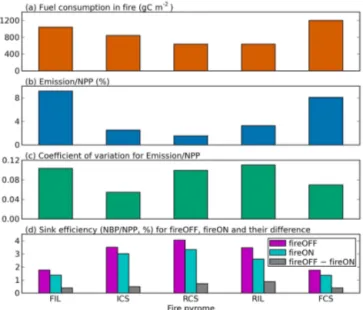
Figure 11.Characteristics of different fire pyromes (defined as by Archibald et al., 2013) in terms of the role of fires in the terres-trial carbon balance.(a)Fuel consumption in fire;(b) emissions as percentage of NPP;(c)coefficient of variation for the ratio of emissions against NPP; and(d) sink efficiencies (i.e. NBP/NPP) for fireOFF and fireON simulations and their difference. All vari-ables are shown for 1901–2012, except the fuel carbon consump-tion, which is averaged over 2003–2012. The five fire pyromes are FIL, frequent–intense–large; ICS, intermediate–cool–small; RCS, rare–cool–small; RIL, rare–intense–large; and FCS, frequent–cool– small. Refer to Fig. S2 for their spatial distributions.
the two studies are similar (1.9 Pg C yr−1by both studies for
the twentieth century). Therefore, the difference in fire sink reduction between the two studies must be due to differences in other flux estimates (NPP and heterotrophic respiration).
Li et al. (2014) estimated that fire reduced global NPP by 1.9 Pg C yr−1, but the heterotrophic respiration was re-duced by an even larger amount (2.7 Pg C yr−1), resulting in a higher NEP of 0.9 Pg C yr−1 in their fire-off simula-tion (called the fire indirect effect). We also find a higher heterotrophic respiration in our fireOFF simulation (by on average 1.62 Pg C yr−1over 1901–2012), but the simulated NPP difference is negligible (6 Tg C yr−1higher in fireOFF than fireON). The NPP reduction by fire is probably underes-timated in our study, because land-cover change fires are not accounted for, and grassland or agricultural land converted from forest has much lower NPP than it had prior to con-version (Houghton et al., 1999). Thus the NEP increase by switching fire off might also be underestimated, which leads to underestimated sink reduction by fire.
out that if all fires were suppressed, tree cover would ex-pand in regions where current grassland or woodland ecosys-tems are maintained by fires (Bond et al., 2005; Staver et al., 2011), and that the expanded forest coverage would increase land carbon stock (Bond et al., 2005). Secondly, because OR-CHIDEE was not coupled to an atmosphere model, the atmo-spheric concentration changes for various gases released by fire, or a complete fire–vegetation–climate feedback, as dis-cussed in the Introduction, were not included.
3.3.5 The role of fires in the terrestrial carbon balance in relation to fire pyromes
We compared fire fuel consumption, the fraction of NPP re-turned via fire emissions and its temporal variation, and car-bon sink efficiencies (SE) for fireOFF and fireON simula-tions for the five pyromes defined by Archibald et al. (2013) (see Sect. 2.5). The temporal variation for the fraction of NPP lost to fire emissions is examined as the coefficient of vari-ation during 1901–2012, which is the standard devivari-ation di-vided by the mean.
According to model simulation, frequent–intense–large (FIL) and frequent–cool–small (FCS) fires have higher fuel consumption than infrequent rare–intense–large (RIL) and rare–cool–small (RCS) fires (Fig. 11), fuel consumption be-ing highest in the FCS pyrome (1.2 kg C m−2)and lowest in the RCS pyrome (0.6 kg C m−2). Correspondingly, the ratio of fire emissions to NPP is also higher in frequent-fire py-romes than in infrequent ones, but the temporal variation of this fraction is higher for the RCS and RIL pyromes. Regions with infrequent fires (RCS, RIL and ICS) have greater sink efficiency than those with frequent ones (FIL, FCS) for the fireOFF simulation. This pattern remains for the fireON sim-ulation, which gives smaller sink efficiency than fireOFF for all the pyromes, due to the adverse effects of fires on the land carbon sink. Consequently, the sink efficiency as reduced by fires remains higher in infrequent-fire pyromes (being high-est in the RIL pyrome) than frequent ones (being lowhigh-est in the FIL pyrome).
It is reasonable to find that frequent fires have higher fuel consumption than small cool ICS and RCS fires, because the latter are generally human-controlled burning with lim-ited fuel load (Archibald et al., 2013). However, intuitively, the rare–intense–large (RIL) fires are expected to have at least comparable, if not larger, fuel consumption than the FIL and FCS pyromes, since their spatial extent covers the North American boreal forest biome where large amounts of soil (and biomass) carbon stocks are exposed to burn-ing. Our model simulation does show a high amount of fire fuel consumption in North American boreal forests: 1–5 kg C m−2(Fig. 5), comparable to that reported in regional stud-ies (French et al., 2011; Kasischke and Hoy, 2012). A closer examination of the fire pryome distribution map (Fig. S2) reveals that some of the grassland fires in central and east-ern Asia and inland Australia are also classified as RIL fires,
which have a rather low simulated fuel consumption rate (1– 200 g C m−2, Fig. 5). Thus the simulated fuel consumption
for RIL fires is a mean value for all the above regions (in-cluding boreal forests in Eurasia as well), which is lower than frequent fires.
We also find that the carbon sink efficiencies for infrequent-fire pyromes are higher than frequent ones for both fireON and fireOFF simulations, probably because more forests are located in infrequent-fire pyromes (Table 1 in Archibald et al., 2013). The sink efficiency reduction (SEOFF−SEON)by fires is highest in the RIL pyrome,
con-gruent with a higher emission-to-NPP fraction. If we exam-ine the percentage of fire-induced sink efficiency reduction to SEOFF, the FIL, FCS and RIL pyromes emerge again to have
a higher percentage than the RCS and ICS pyromes (data not shown). This indicates that frequent fires and infrequent large fires reduce the carbon sequestration capacity of land ecosystems to a higher extent. Note that as an initial attempt to understand the role of fires in carbon cycling for different pyromes (such as that for different biomes), great uncertain-ties exist in the modelling results presented here. Sources of uncertainties include the fact that agricultural and deforesta-tion fires were included in Archibald et al. (2013) but not in our model; errors and uncertainties exist in simulated fire fuel consumption and fire emissions; the combustion difference between surface fires in boreal Eurasian forests and crown fires in North American boreal forests (de Groot et al., 2013; Wirth, 2005) is lacking in the model; and uncertainties exist in the classification of fire pyromes.
4 Summary and conclusions
In this study, we used the ORCHIDEE land surface model with the recently integrated SPITFIRE model to estimate the role of fires in the terrestrial carbon balance for the twenti-eth century. The simulated global fire carbon emissions for 1997–2009 are 2.1 Pg C yr−1, close to the 2.0 Pg C yr−1as estimated by the GFED3.1 data (when all types of fires are included), owing to error compensation among different re-gions in the model. Fire carbon emissions are mainly under-estimated in Southern Hemisphere tropical regions and this error is compensated for by an overestimation in temperate ecosystems. The regional emission errors are found to be co-incident with the errors in simulated burned areas, with the exception that fire fuel consumption is underestimated in re-gions featuring peatland or deforestation fires such as equa-torial Asia, because these fires are not explicitly included in the model.
years mainly compensate for heterotrophic respiration that would occur without fire combustion, but emissions in ex-treme high fire years far exceed their respiration partial com-pensation and create a larger reduction in the terrestrial car-bon sink. This fire-induced sink reduction has been found to be significantly correlated with climatic variations, includ-ing El Niño–Southern Oscillation (ENSO), with larger sink reductions occurring in warm, dry conditions. This finding has an important implication for the future role of fires in the terrestrial carbon balance, because the capacity of terres-trial ecosystems to sequester carbon will be more likely di-minished in a future climate with more frequent and intense droughts and more extreme El Niño events. This also im-plies that fires might significantly impact the climate–carbon response (known as the γ factor) as simulated by coupled climate–carbon models.
The Supplement related to this article is available online at doi:10.5194/gmd-8-1321-2015-supplement.
Acknowledgements. We thank S. Archibald for providing the fire pyrome distribution map. Moreover, we thank the two anonymous reviewers for providing valuable comments which improved the quality of the manuscript. Funding for this work was provided by the ESA firecci project (http://www.esa-fire-cci.org/) and EU FP7 project PAGE21.
Edited by: D. Lawrence
References
Archibald, S., Lehmann, C. E. R., GómezsDans, J. L., and Bradstock, R. A.: Defining pyromes and global syndromes of fire regimes, Proc. Natl. Acad. Sci. USA, 110, 6442–6447, doi:10.1073/pnas.1211466110, 2013.
Balshi, M. S., McGuire, A. D., Duffy, P., Flannigan, M., Kick-lighter, D. W., and Melillo, J.: Vulnerability of carbon storage in North American boreal forests to wildfires during the 21st cen-tury, Global Change Biol., 15, 1491–1510, 2009.
Beck, P. S. A., Goetz, S. J., Mack, M. C., Alexander, H. D., Jin, Y., Randerson, J. T., and Loranty, M. M.: The impacts and im-plications of an intensifying fire regime on Alaskan boreal forest composition and albedo, Global Change Biol., 17, 2853–2866, doi:10.1111/j.1365-2486.2011.02412.x, 2011.
Bond, W. J., Woodward, F. I., and Midgley, G. F.: The global distri-bution of ecosystems in a world without fire, New Phytol., 165, 525–537, doi:10.1111/j.1469-8137.2004.01252.x, 2005. Bowman, D. M. J. S., Balch, J. K., Artaxo, P., Bond, W. J., Carlson,
J. M., Cochrane, M. A., D’Antonio, C. M., DeFries, R. S., Doyle, J. C., Harrison, S. P., Johnston, F. H., Keeley, J. E., Krawchuk, M. A., Kull, C. A., Marston, J. B., Moritz, M. A., Prentice, I. C., Roos, C. I., Scott, A. C., Swetnam, T. W., van der Werf, G. R., and Pyne, S. J.: Fire in the Earth System, Science, 324, 481–484, doi:10.1126/science.1163886, 2009.
Cai, W., Borlace, S., Lengaigne, M., van Rensch, P., Collins, M., Vecchi, G., Timmermann, A., Santoso, A., McPhaden, M. J., Wu, L., England, M. H., Wang, G., Guilyardi, E., and Jin, F.-F.: Increasing frequency of extreme El Nino events due to greenhouse warming, Nature Clim. Change, 4, 111–116, doi:10.1038/nclimate2100, 2014.
Carmona-Moreno, C., Belward, A., Malingreau, J.-P., Hartley, A., Garcia-Alegre, M., Antonovskiy, M., Buchshtaber, V., and Pivo-varov, V.: Characterizing interannual variations in global fire cal-endar using data from Earth observing satellites, Global Change Biol., 11, 1537–1555, doi:10.1111/j.1365-2486.2005.01003.x, 2005.
Chen, Y., Randerson, J. T., Morton, D. C., DeFries, R. S., Col-latz, G. J., Kasibhatla, P. S., Giglio, L., Jin, Y., and Marlier, M. E.: Forecasting Fire Season Severity in South America Us-ing Sea Surface Temperature Anomalies, Science, 334, 787–791, doi:10.1126/science.1209472, 2011.
Chuvieco, E., Giglio, L., and Justice, C.: Global characterization of fire activity: toward defining fire regimes from Earth observation data, Global Change Biol., 14, 1488–1502, 2008.
De Groot, W. J., Cantin, A. S., Flannigan, M. D., Soja, A. J., Gow-man, L. M., and Newbery, A.: A comparison of Canadian and Russian boreal forest fire regimes, Forest Ecol. Manag., 294, 23– 34, doi:10.1016/j.foreco.2012.07.033, 2013.
Dufresne, J.-L., Foujols, M.-A., Denvil, S., Caubel, A., Marti, O., Aumont, O., Balkanski, Y., Bekki, S., Bellenger, H., Benshila, R., Bony, S., Bopp, L., Braconnot, P., Brockmann, P., Cadule, P., Cheruy, F., Codron, F., Cozic, A., Cugnet, D., Noblet, N. de, Duvel, J.-P., Ethé, C., Fairhead, L., Fichefet, T., Flavoni, S., Friedlingstein, P., Grandpeix, J.-Y., Guez, L., Guilyardi, E., Hauglustaine, D., Hourdin, F., Idelkadi, A., Ghattas, J., Jous-saume, S., Kageyama, M., Krinner, G., Labetoulle, S., Lahel-lec, A., Lefebvre, M.-P., Lefevre, F., Levy, C., Li, Z. X., Lloyd, J., Lott, F., Madec, G., Mancip, M., Marchand, M., Masson, S., Meurdesoif, Y., Mignot, J., Musat, I., Parouty, S., Polcher, J., Rio, C., Schulz, M., Swingedouw, D., Szopa, S., Talandier, C., Terray, P., Viovy, N., and Vuichard, N.: Climate change projections us-ing the IPSL-CM5 Earth System Model: from CMIP3 to CMIP5, Clim. Dynam., 40, 2123–2165, doi:10.1007/s00382-012-1636-1, 2013.
Fang, J., Chen, A., Peng, C., Zhao, S., and Ci, L.: Changes in For-est Biomass Carbon Storage in China Between 1949 and 1998, Science, 292, 2320–2322, doi:10.1126/science.1058629, 2001. Fernandes, P. M., Davies, G. M., Ascoli, D., Fernández, C.,
Mor-eira, F., Rigolot, E., Stoof, C. R., Vega, J. A., and Molina, D.: Prescribed burning in southern Europe: developing fire manage-ment in a dynamic landscape, Front. Ecol. Environ., 11, e4–e14, doi:10.1890/120298, 2013.
Field, R. D., van der Werf, G. R., and Shen, S. S. P.: Human ampli-fication of drought-induced biomass burning in Indonesia since 1960, Nat. Geosci., 2, 185–188, doi:10.1038/ngeo443, 2009. Flannigan, M. D., Krawchuk, M. A., de Groot, W. J., Wotton, B. M.,
and Gowman, L. M.: Implications of changing climate for global wildland fire, Int. J. Wildland Fire, 18, 483–507, 2009.
emis-sions from North American wildland fire, J. Geohys. Res., B, 116, G00K05, doi:10.1029/2010JG001469, 2011.
Giglio, L., Randerson, J. T., van der Werf, G. R., Kasibhatla, P. S., Collatz, G. J., Morton, D. C., and DeFries, R. S.: Assess-ing variability and long-term trends in burned area by mergAssess-ing multiple satellite fire products, Biogeosciences, 7, 1171–1186, doi:10.5194/bg-7-1171-2010, 2010.
Gill, A. M. and Allan, G.: Large fires, fire effects and the fire-regime concept, Int. J. Wildland Fire, 17, 688–695, 2008.
Hayes, D. J., McGuire, A. D., Kicklighter, D. W., Gurney, K. R., Burnside, T. J., and Melillo, J. M.: Is the northern high-latitude land-based CO2 sink weakening?, Global Biogeochem. Cycles, 25, GB3018, doi:10.1029/2010GB003813, 2011.
Hoffmann, W. A., Geiger, E. L., Gotsch, S. G., Rossatto, D. R., Silva, L. C., Lau, O. L., Haridasan, M., and Franco, A. C.: Ecological thresholds at the savanna-forest boundary: how plant traits, resources and fire govern the distribution of tropical biomes, Ecol. Lett., 15, 759–768, 2012.
Houghton, R. A., Hackler, J. L., and Lawrence, K. T.: The U.S. Carbon Budget: Contributions from Land-Use Change, Science, 285, 574–578, doi:10.1126/science.285.5427.574, 1999. Jin, Y., Randerson, J. T., Goetz, S. J., Beck, P. S. A., Loranty, M. M.,
and Goulden, M. L.: The influence of burn severity on postfire vegetation recovery and albedo change during early succession in North American boreal forests, J. Geohys. Res., B, 117, G01036, doi:10.1029/2011JG001886, 2012.
Jung, M., Reichstein, M., Margolis, H. A., Cescatti, A., Richardson, A. D., Arain, M. A., Arneth, A., Bernhofer, C., Bonal, D., Chen, J., Gianelle, D., Gobron, N., Kiely, G., Kutsch, W., Lasslop, G., Law, B. E., Lindroth, A., Merbold, L., Montagnani, L., Moors, E. J., Papale, D., Sottocornola, M., Vaccari, F., and Williams, C.: Global patterns of land-atmosphere fluxes of carbon dioxide, la-tent heat, and sensible heat derived from eddy covariance, satel-lite, and meteorological observations, J. Geohys. Res., B, 116, G00J07, doi:10.1029/2010JG001566, 2011.
Kasischke, E. S. and Hoy, E. E.: Controls on carbon consumption during Alaskan wildland fires, Global Change Biol., 18, 685– 699, doi:10.1111/j.1365-2486.2011.02573.x, 2012.
Keeley, J. E., Fotheringham, C. J., and Morais, M.: Reexamining Fire Suppression Impacts on Brushland Fire Regimes, Science, 284, 1829–1832, doi:10.1126/science.284.5421.1829, 1999. Kelly, R., Chipman, M. L., Higuera, P. E., Stefanova, I., Brubaker,
L. B., and Hu, F. S.: Recent burning of boreal forests exceeds fire regime limits of the past 10,000 years, Proc. Natl. Acad. Sci. USA, 110, 13055–13060, doi:10.1073/pnas.1305069110, 2013. Kiladis, G. N. and Diaz, H. F.: Global Climatic
Anoma-lies Associated with Extremes in the Southern Oscil-lation, J. Climate, 2, 1069–1090, doi:10.1175/1520-0442(1989)002<1069:GCAAWE>2.0.CO;2, 1989.
Kitzberger, T., Swetnam, T. W., and Veblen, T. T.: Inter-hemispheric synchrony of forest fires and the El Niño-Southern Oscilla-tion, Global Ecol. Biogeogr., 10, 315–326, doi:10.1046/j.1466-822X.2001.00234.x, 2001.
Kloster, S., Mahowald, N. M., Randerson, J. T., Thornton, P. E., Hoffman, F. M., Levis, S., Lawrence, P. J., Feddema, J. J., Ole-son, K. W., and Lawrence, D. M.: Fire dynamics during the 20th century simulated by the Community Land Model, Biogeo-sciences, 7, 1877–1902, doi:10.5194/bg-7-1877-2010, 2010.
Kloster, S., Mahowald, N. M., Randerson, J. T., and Lawrence, P. J.: The impacts of climate, land use, and demography on fires during the 21st century simulated by CLM-CN, Biogeosciences, 9, 509–525, doi:10.5194/bg-9-509-2012, 2012.
Krinner, G., Viovy, N., de Noblet-Ducoudré, N., Ogée, J., Polcher, J., Friedlingstein, P., Ciais, P., Sitch, S., and Prentice, I. C.: A dynamic global vegetation model for studies of the coupled atmosphere-biosphere system, Global Biogeochem. Cycles, 19, GB1015, doi:10.1029/2003GB002199, 2005.
Langenfelds, R. L., Francey, R. J., Pak, B. C., Steele, L. P., Lloyd, J., Trudinger, C. M., and Allison, C. E.: Interannual growth rate variations of atmospheric CO2 and itsδ13C, H2, CH4, and CO
between 1992 and 1999 linked to biomass burning, Global Bio-geochem. Cycles, 16, 21-1–21-22, doi:10.1029/2001GB001466, 2002.
Le Quéré, C., Andres, R. J., Boden, T., Conway, T., Houghton, R. A., House, J. I., Marland, G., Peters, G. P., van der Werf, G. R., Ahlström, A., Andrew, R. M., Bopp, L., Canadell, J. G., Ciais, P., Doney, S. C., Enright, C., Friedlingstein, P., Huntingford, C., Jain, A. K., Jourdain, C., Kato, E., Keeling, R. F., Klein Gold-ewijk, K., Levis, S., Levy, P., Lomas, M., Poulter, B., Raupach, M. R., Schwinger, J., Sitch, S., Stocker, B. D., Viovy, N., Zaehle, S., and Zeng, N.: The global carbon budget 1959–2011, Earth Syst. Sci. Data, 5, 165–185, doi:10.5194/essd-5-165-2013, 2013. Li, F., Levis, S., and Ward, D. S.: Quantifying the role of fire in the Earth system – Part 1: Improved global fire modeling in the Community Earth System Model (CESM1), Biogeosciences, 10, 2293–2314, doi:10.5194/bg-10-2293-2013, 2013.
Li, F., Bond-Lamberty, B., and Levis, S.: Quantifying the role of fire in the Earth system – Part 2: Impact on the net carbon balance of global terrestrial ecosystems for the 20th century, Biogeo-sciences, 11, 1345–1360, doi:10.5194/bg-11-1345-2014, 2014. Liu, H. and Randerson, J. T.: Interannual variability of
sur-face energy exchange depends on stand age in a boreal forest fire chronosequence, J. Geophys. Res., 113, G01006, doi:10.1029/2007JG000483, 2008.
Liu, J., Wang, B., Cane, M. A., Yim, S.-Y., and Lee, J.-Y.: Divergent global precipitation changes induced by nat-ural versus anthropogenic forcing, Nature, 493, 656–659, doi:10.1038/nature11784, 2013.
Luyssaert, S., Ciais, P., Piao, S. L., Schulze, E.-D., Jung, M., Za-ehle, S., Schelhaas, M. J., Reichstein, M., Churkina, G., Papale, D., Abril, G., Beer, C., Grace, J., Loustau, D., Matteucci, G., Magnani, F., Nabuurs, G. J., Verbeeck, H., Sulkava, M., Van Der WERF, G. R., Janssens, I. A., and Team members of the C.-I. S.: The European carbon balance. Part 3: forests, Global Change Biol., 16, 1429–1450, doi:10.1111/j.1365-2486.2009.02056.x, 2010.
Mack, M. C., Bret-Harte, M. S., Hollingsworth, T. N., Jandt, R. R., Schuur, E. A. G., Shaver, G. R., and Verbyla, D. L.: Carbon loss from an unprecedented Arctic tundra wildfire, Nature, 475, 489– 492, doi:10.1038/nature10283, 2011.
Magi, B. I., Rabin, S., Shevliakova, E., and Pacala, S.: Separat-ing agricultural and non-agricultural fire seasonality at regional scales, Biogeosciences, 9, 3003–3012, doi:10.5194/bg-9-3003-2012, 2012.