NUNO MIGUEL MATIAS CARVALHAIS

(1)

NUNO MIGUEL MATIAS CARVALHAIS

IBERIAN PENINSULA ECOSYSTEM CARBON FLUXES

:

A

MODEL-DATA

INTEGRATION

STUDY

Dissertação apresentada para obtenção do Grau de Doutor em Engenharia do Ambiente pela Universidade Nova de Lisboa,

Faculdade de Ciências e Tecnologia.

LISBOA 2010

UNIÃO EUROPEIA

(2)

(3)

(4)

(5)

Acknowledgments

At this point, many names come up to my mind for a multitude of reasons; almost constantly

these mix between professional and personal motives, which are hardly distinguishable.

Júlia Seixas, my supervisor, for the initial challenge to do research and later a PhD in her

group, and for the freedom to go my own way.

A bit out of the track of my PhD, but strongly influential, I would like to mention: Ricardo

Ribeiro, for the always motivating discussions; Pete Loucks, for inviting and wonderfully

receiving a group of us for a stay at Cornell University; and Wilhelmina Clavano, for the

discussions around a froggie.

Jim Tucker, for the invitation to visit the GIMMS group, in the Goddard Space Flight Center,

giving me the opportunity to work and learn about remote sensing with his fantastic team.

Ana Pinheiro and Jeff Privette were great hosts that easily juggled between scientific and

house-hunting advises. Jorge Pinzon and Dan Slayback, that strongly support the production

of the GIMMS NDVI dataset and were also available for whatever questions would come up.

Ed Pak, that patiently dealt – and still does sometimes – with my doubts on technical aspects

of the datasets. Assaf Anyamba, for keeping the ELI up and running. And Chris Neigh, a

companion in science, always with an open door. Guido van der Werf provided me with the

very first CASA version I used. Also, Chris Field and George Merchant, which made

available their version of the CASA model as well. Jim Collatz, whom I met while in my first

stay in Goddard, that became a crucial contributor and critic of my work, always keeping me

on my toes.

Ranga Myneni, for giving me the opportunity to learn remote sensing with him and Yuri

Knyazikhin at his group in Boston University, and for amicably receiving me. In Boston, the

coffee and cigarette breaks, lunches and dinners with Wenze Yang, Sangram Ganguly and

Miina Rautiainen surely made research at BU – and the life around Commonwealth Avenue –

a much more eclectic experience.

(6)

I am especially grateful to Markus Reichstein, for the support and motivation, for the

inevitably endless and chaotic discussions, for the hard questions, for crunching code and

beers. Unquestionably, a crucial influence in my pathway during my PhD. I am deeply

thankful for the opportunity to work with him and with the Model-Data Integration group, at

the Max Planck Institute for Biogeochemistry, in Jena, and for opening me the door to the

scientific community.

At the BGC-MDI group I found an extraordinary cooperative and working environment. I

have to mention in particular: Miguel Mahecha, for the openness and the constant

confrontational ideas; Gitta Lasslop, for her almost constant availability for fruitful discussion

and the sharp supportive and critical views; Enrico Tomelleri, for being collaborative and

always ready for a spontaneous frenzy of questions; and Martin Jung, that helped clearing out

ideas in the midst of the smoke of many cigarettes. Andreas Kramer, Peer Koch and Birgitta

Wiehl, whose dedication grants a warm hospitality and fantastic working conditions, from

computing to secretariat support, during my frequent stays at the MPI.

Philippe Ciais, for his interest and for his questions in general, and for asking “what about the

wood?” in particular.

Conceição Capelo and Carina Gomes, for the secretariat support at FCT UNL and the positive

attitude whenever bureaucracy issues or short-notice requests would pop up.

Nuno Pacheco, for always finding a solution for most of the software and hardware issues that

arbitrarily decide to show up; and Akli Benali, that helped with data gathering and handling,

processing and discussing land cover maps.

For being active collaborators in the development of particular aspects of this research that

ended up published or submitted: Akli Benali, Paul Berbigier, Arnaud Carrara, Jim Collatz,

Philippe Ciais, André Granier, Miguel Mahecha, Mirco Migliavacca, Leonardo Montagnani,

Chris Neigh, Dario Papale, Serge Rambal, Markus Reichstein, João Santos Pereira, María

José Sanz, Júlia Seixas, Enrico Tomelleri and Riccardo Valentini.

For reading and/or discussing parts or the full extent of the introductory component of the

dissertation: Ana Cristina Carvalho, Anna Görner, Augusta Costa Sousa, Carlota Lavinas,

Chris Neigh, Gitta Lasslop, João Pedro Nunes, Júlia Seixas, Markus Reichstein, Mirco

(7)

Nuno Grosso, Pedro Lourenço and João Pedro Nunes are my comrades. Through these years,

many discussions about details of my work – but mostly not only – have passed through, or

just blasted on, them. They have replied to and with enough amounts of entropy.

The wisdom and the truly unconditional support from my father, my mother and my sister,

Domingos, Marília and Sara, have been, and will always be, fundamental.

To Carlota Lavinas I could try, but would never be able, to express myself with words.

This work was supported by the Portuguese Foundation for Science and Technology (FCT),

the European Union under Operational Program “Science and Innovation” (POCI 2010), PhD

grant ref. SFRH/BD/6517/2001, co-sponsored by the European Social Fund. Further support,

concerning the final months of the PhD, was provided by a Max Planck Society research

(8)

(9)

Abstract

Terrestrial ecosystems play a key role within the context of the global carbon cycle.

Characterizing and understanding ecosystem level responses and feedbacks to climate drivers

is essential for diagnostic purposes as well as climate modelling projections. Consequently,

numerous modelling and data driven approaches emerge, aiming the appraisal of

biosphere-atmosphere carbon fluxes. The combination of biogeochemical models with observations of

ecosystem carbon fluxes in a model-data integration framework enables the recognition of

potential limitations of modelling approaches. In this regard, the steady-state assumption

represents a general approach in the initialization routines of biogeochemical models that

entails limitations in the ability to simulate net ecosystem fluxes and in model development

exercises.

The present research addresses the generalized assumption of initial steady-state conditions in

ecosystem carbon pools for modelling carbon fluxes of terrestrial ecosystems, from local to

regional scales. At local scale, this study aims to evaluate the implications of equilibrium

assumptions on modelling performance and on optimized parameters and uncertainty

estimates based on a model-data integration approach. These results further aim to support the

estimates of regional net ecosystem fluxes, following a bottom-up approach, by focusing on

parameters governing net primary production (NPP) and heterotrophic respiration (RH)

processes, which determine the simulation of the net ecosystem production fluxes in the

CASA model. An underlying goal of the current research is addressed by focusing on

Mediterranean ecosystem types, or ecosystems potentially present in Iberia, and evaluate the

general ability of terrestrial biogeochemical models in estimating net ecosystem fluxes for the

Iberian Peninsula region. At regional scales, and given the limited information available, the

main objective is to minimize the implications of the initial conditions in the evaluation of the

temporal dynamics of net ecosystem fluxes.

Inverse model parameter optimizations at site level are constrained by eddy-covariance

measurements of net ecosystem fluxes and driven by local observations of meteorological

variables and vegetation biophysical variables from remote sensing products. Optimizations

(10)

parameter uncertainties when compared to optimizations under relaxed initial conditions. In

addition, assuming initial steady-state conditions tend to bias parameter retrievals – reducing

NPP sensitivity to water availability and RH responses to temperature – in order to prescribe

sink conditions. But nonequilibrium conditions can be experienced in soil and/or vegetation

carbon pools under alternative underlying dynamics, which are solely discernible through the

integration of additional information sources, circumventing equifinality issues. Overall,

model performance yields significant results throughout site level optimizations, supporting

the regional estimates ecosystem fluxes for the Iberian Peninsula, despite a lower

representativeness is observed in the North-western region. Although a sensitivity analysis

shows significant impacts of initial conditions in the time series of net ecosystem fluxes, a

method is proposed to estimate inter-annual variability and temporal trends

quasi-independently from the initial conditions. A deeper evaluation of net ecosystem production

trends reveals the significant role of primary production in driving positive trends in northern

and western regions; and the role of trends allocation strategies (driven by water availability)

in explaining negative trends in the southern central regions. The link between assimilatory

fluxes and net ecosystem fluxes is established in both positive and negative trends regions.

These results emphasizes that the underlying mechanisms of trends in net ecosystem fluxes

are strongly associated with primary production and allocation processes.

In general, challenging the model components is informative on the mechanisms and

parameters behind the variability in net ecosystem fluxes that are amenable for

regionalization. The initial conditions are a fundamental component throughout model

development and application activities, since equilibrium assumptions limit model

optimization and performance on local scales, as well as temporal trends assessment on

regional domains. Hence, the robustness of a bottom-up modelling exercise also stems from

the ability to infer simulated dynamics disassociated from initial equilibrium assumptions.

Ultimately, the present work emphasizes the relevance of addressing general assumptions of

(11)

Resumo

Os ecossistemas terrestres desempenham um papel fundamental no contexto do ciclo global

do carbono. A caracterização e compreensão de respostas e feedbacks dos fluxos de carbono

terrestres a variáveis climáticas são essenciais para exercícios de modelação. Em

consequência, observa-se o aparecimento de várias abordagens baseadas em modelação e/ou

em dados medidos localmente, que visam a avaliação de fluxos de carbono entre a biosfera e a

atmosfera. A comparação de modelos biogeoquímicos com medições de fluxos de carbono em

ecossistemas terrestres, numa estrutura de integração de modelos e dados, permite o

reconhecimento de potenciais limitações da modelação. Nesta perspectiva, a consideração de

condições iniciais de equilíbrio ao nível dos reservatórios de carbono do ecossistema constitui

um procedimento comum, com potenciais implicações na estimativa de fluxos líquidos de

carbono e no desenvolvimento de modelos em geral.

O presente trabalho aborda as implicações da assumpção de condições iniciais de equilíbrio

nos reservatórios de carbono de ecossistemas terrestres num contexto de modelação de fluxos

de carbono entre o ecossistema e a atmosfera, com ênfase à escala local e regional. À escala

local, este estudo visa a análise das implicações da consideração de equilíbrio, tanto a nível do

desempenho da modelação, como na estimativa de parâmetros e respectiva incerteza,

baseando-se no modelo Carnegie-Ames-Stanford Approach (CASA).

Esta parametrização visa suportar a posterior simulação dos fluxos de carbono à escala

regional, seguindo uma abordagem bottom-up, visto focar a optimização de parâmetros

reguladores da produtividade primária líquida e da respiração heterotrófica – processos

determinantes da produtividade líquida do ecossistema simulados pelo modelo CASA. Um

objectivo subjacente ao trabalho apresentado centra-se na capacidade dos modelos

biogeoquímicos terrestres para simular os fluxos de carbono em ecossistemas Mediterrânicos,

ou ecossistemas potencialmente presentes na Península Ibérica. À escala regional, e dadas as

limitações de informação disponível, o principal objectivo é minimizar os efeitos das

condições iniciais na avaliação da dinâmica temporal dos fluxos de carbono do ecossistema.

As medições de fluxos de carbono entre o ecossistema e a atmosfera, através do método de

(12)

exercícios de optimização. Em paralelo, observações das condições meteorológicas locais e

das propriedades biofísicas da vegetação por detecção remota constituem as variáveis

condutoras do modelo. Os resultados da optimização revelam um desempenho superior do

modelo, assim como uma menor incerteza nos parâmetros estimados, quando é permitido o

relaxamento das condições iniciais de equilíbrio, em comparação com condições iniciais de

equilíbrio forçadas. Sob condições de equilíbrio inicial os parâmetros apresentam

enviezamentos compensatórios, a fim de simular as condições de sumidouro observadas a

nível local. Por um lado, a redução da sensibilidade da actividade fotossintética à

disponibilidade hídrica leva ao aumento da taxa assimilatória em períodos stress hídrico. Por

outro lado, a redução da resposta da respiração heterotrófica à temperatura, leva à redução das

emissões resultantes do aumento da actividade respiratória com o aumento da temperatura.

Contudo, condições de (não) equilíbrio podem ser observadas nos diferentes reservatórios de

carbono do ecossistema. No entanto, estas apenas são discerníveis através da integração de

fontes de informação adicionais sobre os reservatórios, contornando questões de

equifinalidade. Em geral, a confiança nas estimativas de fluxos de carbono do ecossistema é

significativa. Desta forma, a simulação de fluxos de carbono para a região da Peninsula

Ibérica assenta no modelo CASA, apesar de uma baixa representatividade para a região

Noroeste. Embora as condições iniciais impliquem impactes significativos nas séries

temporais dos fluxos de carbono, propõe-se um método de correcção que minimiza

consideravelmente o seu efeito na variabilidade inter-anual e nas tendências temporais. A

posterior avaliação detalhada dos fluxos de assimilação e emissão de carbono revela a

dinâmica subjacente às tendências na produtividade líquida do ecossistema. A produtividade

primária líquida, associada à fenologia, é o principal factor responsável pelas tendências

positivas nos fluxos de carbono nas regiões norte e oeste da Península Ibérica. As tendências

negativas nas regiões centro-sul da Península reflectem tendências nas estratégias de alocação

de carbono pela vegetação, e pelo ecossistema, dominadas pela disponibilidade hídrica. A

ligação entre os fluxos assimilatórios é estabelecida em zonas de tendências tanto positivas

como negativas. Estes resultados salientam a importância da produtividade primária e dos

mecanismos de alocação de carbono na avaliação dos fluxos de carbono entre os ecossistemas

terrestres e a atmosfera.

Em geral, a avaliação das diversas componentes dos modelos fornece informação sobre os

mecanismos e parâmetros que controlam a variabilidade dos fluxos de carbono do ecossistema

que são passíveis de regionalização. As condições iniciais representam uma componente

(13)

limitarem tanto a optimização e o desempenho do modelo a escala local, como a estimativa de

tendências temporais a escalas regionais. Neste contexto, a robustez de um exercício de

modelação bottom-up também provém da possibilidade para inferir resultados de simulações

livres de condições iniciais de equilíbrio. Em última análise, o trabalho apresentado ilustra a

relevância da abordagem de pressupostos gerais de modelação em exercícios de integração de

(14)

(15)

Abbreviations

AGB Above-Ground Biomass

AIC Akaike Information Criterion

AICmin Minimum AIC

CASA Carnegie-Ames-Stanford Approach

CASAG Modified CASA model

CFT Cost Function Type

CFM Cost Function with Multiple constraints

CFS Cost Function with a Single constraint

CCSSA Carbon Cycle Steady-State Approach

CCSSAf Fixed Carbon Cycle Steady-State Approach

CCSSAr Relaxed Carbon Cycle Steady-State Approach

CPd Climate-Phenology distance

CW Wood Biomass

DBF Deciduous Broadleaf Forest

EBF Evergreen Broadleaf Forest

ENF Evergreen Needleleaf Forest

EBG Evergreen Broadleaf with Grasses

fAPAR fraction of Absorbed Photosynthetically Active Radiation

fAPART Trend in fAPAR

FST Flux Site

GIMMS Global Inventory Modelling and Mapping Studies

GPP Gross Primary Production

IAV Inter-Annual Variability

IP Iberian Peninsula

LAI Leaf Area Index

LAT Latitude

LON Longitude

MAT Mean Annual Temperature

(16)

MF Mixed Forest

MODIS Moderate Resolution Imaging Spectroradiometer

NBP Net Biome Production

NDVI Normalized Difference Vegetation Index

NAE Normalized Average Error

NMAE Normalized Mean Absolute Error

NEP Net Ecosystem Production

NEPD NEP timeseries decoupled from initial conditions

NEPeq NEP timeseries under initial equilibrium conditions

NEPT Trend in NEP

NPP Net Primary Production

NPPD NPP timeseries decoupled from initial conditions

NPPT Trend in NPP

NPPW Wood NPP

PFT Plant Functional Type

PRM Parameter vector

RA Autotrophic Respiration

RECO Ecosystem Respiration

Rg Solar radiation

RG Growth Respiration

RH Heterotrophic Respiration

D H

R RH timeseries decoupled from initial conditions

RHT Trend in RH

RHeq RH timeseries under initial equilibrium conditions

RM Maintenance Respiration

SA Substrate availability

SAT Trend in SA

SE Standard Error

SHR Shrubland

TAP Total Annual Precipitation

TMR Temporal Resolution

(17)

Symbols

CASA model

Aws Sensitivity of soil turnover rates to water storage

Bwε Sensitivity of ε to water stress

ε Light use efficiency for NPP calculations

ε* Maximum light use efficiency for NPP calculations

εg Light use efficiency for GPP calculations

*

g

 Maximum light use efficiency for GPP calculations

k Soil pools turnover rates

kWR Wood and coarse root turnover rates

Q10 Multiplicative increase in soil biological activity for a 10ºC increase in

temperature

η Steady-state relaxing parameter for soil level pools

η' Steady-state relaxing parameter for soil microbial, slow and old pools ηWL Steady-state relaxing parameter for wood, root and slow litter pools

ηWD Steady-state relaxing parameter for wood under the prescription of a dynamic recovery of the system

ηW Steady-state relaxing parameter for wood and coarse root pools

Ta Temperature sensitivity of ε below Topt

Tb Temperature sensitivity of ε above Topt

Tε Response function of ε to temperature

Topt Optimum temperature for ε

Tref Reference temperature in Q10 function

Ts Response function of soil turnover rates to temperature

(18)

Parameter vectors

0

 Relaxed parameter vector: [ε*, Topt, Bwε, Q10, Aws, η]



k

 Replacing η by k in ₀



Ta

 Replacing η by Ta in 0



Tb

 Replacing η by Tb in 0



Tb

 Replacing η by Tref in 0



*



 Removing ε* from ₀



Topt

 Removing Topt from 0

 

_Bw Removing Bwε from 0



10

Q

 Removing Q10 from 0



Aws

 Removing Aws from 0

 

 Removing η from ₀

emp S

 Empirical relaxation of steady state on decomposition pools (equivalent to₀)

emp SV

 Empirical relaxation of vegetation and some soil pools

mix SV

 Dynamic recovery of vegetation and empirical relaxation some soil pools

dyn V

 Dynamic recovery of vegetation.

dyn Vk

 Dynamic recovery of vegetation adjusting turnover rates (kWR)

emp V

(19)

Authorship

declaration

for

published

work

Part of the work presented in this dissertation is published, in press and submitted in

international peer-reviewed journals:

 Carvalhais, N., Reichstein, M., Seixas, J., Collatz, G.J., Pereira, J.S., Berbigier, P.,

Carrara, A., Granier, A., Montagnani, L., Papale, D., Rambal, S., Sanz, M.J., and

Valentini, R. (2008), Implications of the Carbon Cycle Steady State Assumption for

Biogeochemical Modelling Performance and Inverse Parameter Retrieval, Global

Biogeochemical Cycles, 22, GB2007, doi:10.1029/2007GB003033.

 Carvalhais, N., Reichstein, M., Ciais, P., Collatz, G. J., Mahecha, M. D., Montagnani, L., Papale, D., Rambal, S., and J. Seixas (2010, in press), Identification of Vegetation

and Soil Carbon Pools out of Equilibrium in a Process Model Via Eddy Covariance

and Biometric Constraints, Global Change Biology.

 Carvalhais, N., Reichstein, M., Collatz, G. J., Mahecha, M. D., Migliavacca, M.,

Neigh, C., Tomelleri, E., Benali, A. A., Papale, D., and J. Seixas (submitted),

Deciphering the Components of Regional Net Ecosystem Fluxes Following a

Bottom-up Approach for the Iberian Peninsula, Biogeosciences.

I hereby declare that, as the first author of the above mentioned manuscripts, I provided the

major contribution to the research and technical work developed, to the interpretation of the

(20)

(21)

Table

of

List

of

Figures

Figure 1.1 – Conceptual scheme of the carbon pools, flows and fluxes in the terrestrial

ecosystem component of the global carbon cycle [adapted from Schulze, 2006]. ... 16

Figure 1.2 – Conceptual workflow of a model data integration approach [adapted from

Mahecha, 2009; Williams et al., 2009]... 45

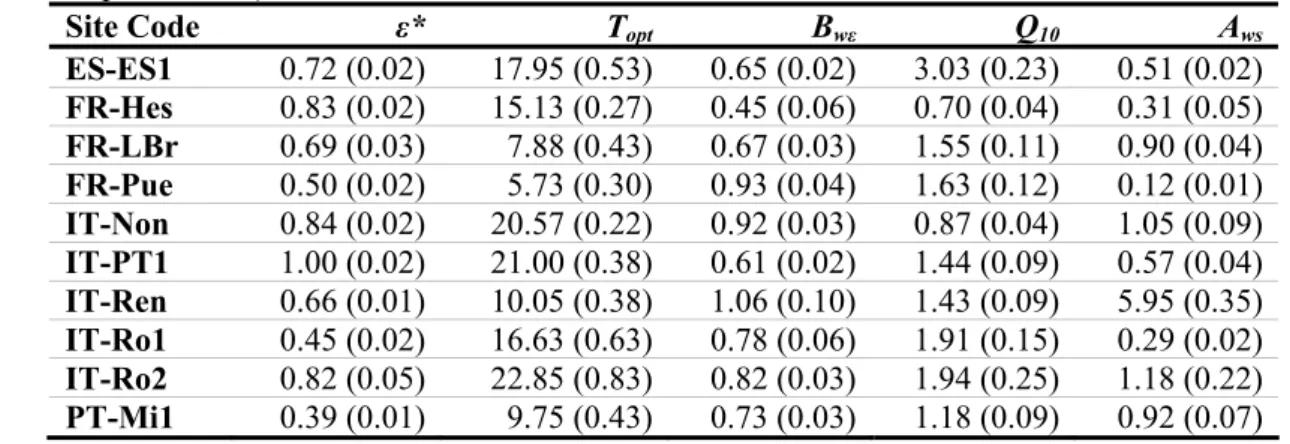
Figure 1.3 – Location and characterization of the Iberian Peninsula in its two most significant

bioclimatic regions: Temperate and Mediterranean [source: EEA, 2008]... 51

Figure 2.1 – ANOVA test results on the four model performance indicators yielded by the

CASA model optimization throughout sites (FST) and temporal resolutions (TMR) for all

parameter sets considered (PRM)... 94

Figure 2.2 – MEF distribution for simulations where η is considered in the parameter set

(CCSSAr). ... 94

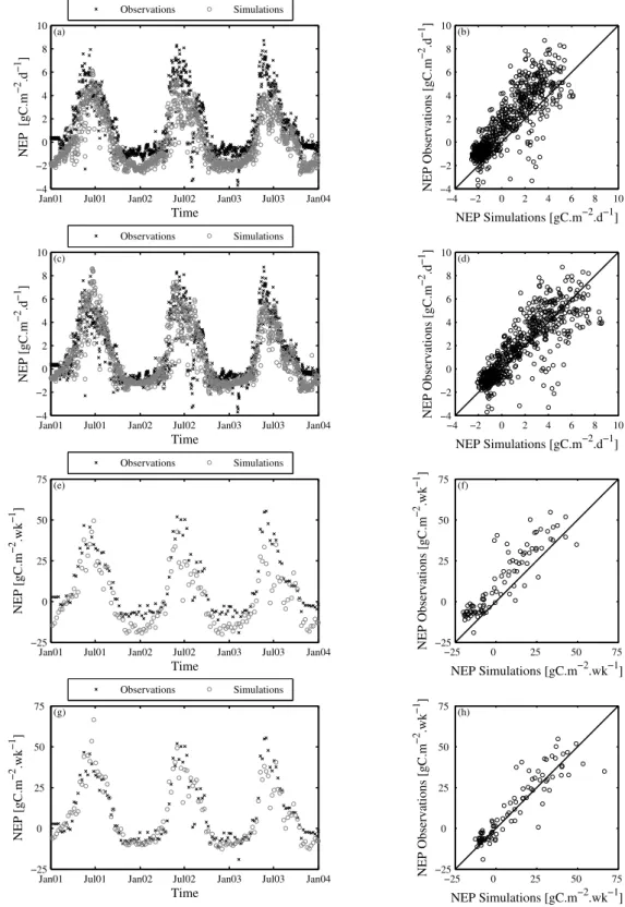
Figure 2.3 – CASA model NEP estimates for IT-Non at different temporal scales... 96

Figure 2.4 – Observations versus simulations results between different parameter sets and ₀

(IT-PT1)... 97

Figure 2.5 – Comparison between model performances of the different parameter sets

considered in the optimization exercise: left – MEF; right – absolute NAE... 98

Figure 2.6 – Relationship between mean annual NEP observations and η optimization results

throughout parameter sets for daily calculations... 99

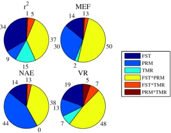
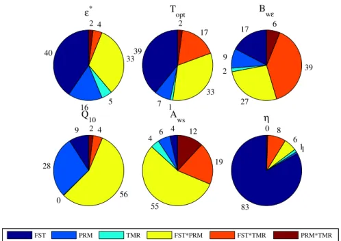
Figure 2.7 – Results of the ANOVA on the optimized parameters variance explained by single

factors and interactions... 100

Figure 2.8 – CCSSAr impact on ε* estimates... 101

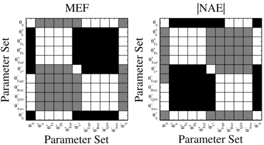
Figure 2.9 – Effects of η in optimized parameter constraints... 102

Figure 2.10 – Results of the ANOVA on the optimized parameters uncertainties variance

explained by single factors and interactions... 104

(28)

primary production (GPP, r2 = 0.96, α < 0.0001) and ecosystem respiration (RECO, r2 = 0.002,

α < 0.91), estimated from flux partitioning...105

Figure 2.12 – Comparison between total soil C pools field measurements (black), estimated by

the CASA model under relaxed (grey) and fix (white) steady-state conditions, considering

different temporal resolutions mean (filled bars) and standard deviation (error bars)...106

Figure 3.1 – The CASA and CASAG scheme of vegetation and soil level carbon pools:

overall, carbon flows from top to bottom...122

Figure 3.2 – Schematic representation of the “mechanistic” experiment principle used in

dynamic recovery setups: dyn V

 , dyn Vk

 and mix

SV

 ; illustrating the evolution of C pools in time

after the prescribed disturbances in vegetation pools...124

Figure 3.3 – ANOVA results for the different model performance indicators used...129

Figure 3.4 – Distribution across sites of model efficiency (MEF) and absolute normalized

average error (|NAE|) ratios between parameter vectors on xx-axis and _Semp...130

Figure 3.5 – Distribution across sites of parameter ratios between parameter vectors on xx-axis

and _Semp. ...131

Figure 3.6 – Distribution of parameter uncertainties ratios between parameter vectors on xx

-axis and _Semp. ...134

Figure 3.7 – Contour plots for single constraint cost functions (NEP) and for the multiple

constraints cost function (NEP, AGB): integrating net ecosystem production fluxes (NEP) and

above ground biomass pools (AGB). ...136

Figure 3.8 – Comparison of NEP MEF between multiple constraint cost functions (CFM –

considering pools and fluxes) and single constraint cost function (CFS – considering fluxes).

...137

Figure 3.9 – The integration of pools in the cost function allows the differentiation between

different model structures by comparison of model efficiency (MEF, left); and allows

identifying model structures that enable the correct simulation of vegetation C pools as well

(right)...138

Figure 3.10 – Comparisons of the model efficiency (MEF) between emp S

 and ηwood parameter

vectors (_SVemp, _SVmix, _Vkdyn and _Vdyn) for optimizations considering solely fluxes in the cost

(29)

(multiple constraint cost function: CFM; 7b). ... 139

Figure 3.11 – Comparison between CASAG model simulations and site observations at

FR-Hes for different experimental setups... 142

Figure 3.12 – Development of vegetation and soil C pools in FR-Pue for three experimental

setups. ... 144

Figure 4.1 – Abacus of NEPT decomposition into NPP and RH trends: NPPT and RHT,

respectively... 164

Figure 4.2 – Spatial patterns of the representativeness of the eddy-covariance sites for pixels

of the Iberian Peninsula. ... 167

Figure 4.3 – The classification of the Iberian Peninsula according to the optimized

eddy-covariance sites per PFT (left column) is based on the selection of the closest site to each

pixel. ... 168

Figure 4.4 – Influence of distance to equilibrium (η) in the inter-annual variability (IAV) in

net ecosystem fluxes (a) and in the IAV in the de-trended NEP fluxes (removing the sole

recovery from the C pools) (b). ... 169

Figure 4.5 – Influence of distance to equilibrium (η) in the IAV in heterotrophic respiration

(RH) fluxes (a) and in the IAV in the de-trended RH fluxes (R , removing the sole recovery DH

from the C pools) (b). ... 170

Figure 4.6 – The distribution of the NEP trends (Sen slopes, gC.m-2.yr-2) is strongly dependent

on η values (a) while for NEPD its distribution appears invariant with η (b). ... 171

Figure 4.7 – Mean significant trends in NEPD, NPPD and R (gC.mD_H -2.yr-2)... 172

Figure 4.8 – Decomposition of NEPD trends into R and NPPD_H D trends (NEP , _TD RH and D_T

D T

NPP , respectively – gC.m-2.yr-2) (a)... 173

Figure 4.9 – Decomposition of NPPD trends (gC.m-2.yr-2) into T_ε and fAPAR trends, TεT and

fAPART, respectively (fractional units per square meter per year) (a)... 174

Figure 4.10 – Decomposition of NPPD trends (gC.m-2.yr-2) into W_ε and fAPAR trends, WεT

and fAPART, respectively (fractional units per square meter per year) (a)... 175

Figure 4.11 – Decomposition of D H

R trends (gC.m-2.yr-2) into Ts and substrate availability

(30)

Figure 4.12 – Decomposition of R trends (gC.mD_H -2.yr-2) into Ws and substrate availability

(SA) trends, WsT and SAT, respectively (fractional units per square meter per year) (a)...176

Figure I.1 – MODIS fAPAR time series resulting from different treatment methods. ...202

Figure II.1 – Effect of optimum temperature (Topt) on light use efficiency estimates. ...206

Figure II.2 – Impact of the Q10 parameter on the effect of temperature on soil biological

activity (Ts)...208

Figure II.3 – Sensitivity of the below ground soil moisture effect (Ws) to the water storage to

monthly PET ratio (Bgr) for different Aws estimates (Ts)...209

Figure V.1 – Changes between _Vemp and _ model efficiency (MEF; left) and normalized

average error (NAE; right) by integrating a parameter that only affects the slow turnover

vegetation pools after equilibrium (ηW in _Vemp)...220

Figure V.2 – Comparison of model performance statistics between CASAG and CASA: a)

normalized average error (NAE); and 2) modelling efficiency (MEF). ...221

Figure V.3 – Relationship between CASA and CASAG maximum light use efficiency

estimates – ε* and *_g, respectively – (a), and CUE for CASAG (b). ...222

(31)

List

of

Tables

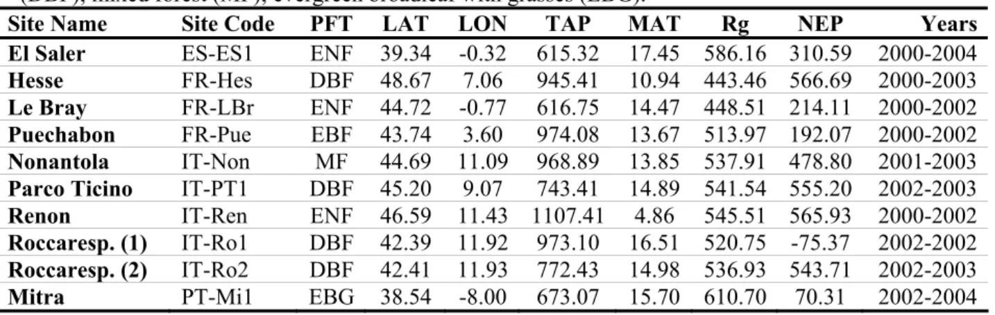
Table 2.1 – Identification of the different sites included in the parameter optimization

analysis. ... 86

Table 2.2 – Parameters used in the different model optimizations. ... 90

Table 2.3 – Identification of the different parameters included in each parameter set. ... 91

Table 2.4 – Model performance results for different temporal resolutions (mean ± standard

deviation). ... 93

Table 2.5 – Frequency of correlation degrees at different temporal resolutions of correlation

matrix results from parameter optimization. ... 95

Table 2.6 – Parameter optimizations results for ₀ at daily temporal scale per site (parameters

standard errors in parentheses). ... 101

Table 2.7 – Results for the parameters’ standard errors (SE) mean and standard deviation

considering both a fix CCSSA (CCSSAf) and a relaxed CCSSA (CCSSAr). ... 104

Table 3.1 – Results for the parameters’ standard errors (SE) mean and standard deviation

considering both a fix CCSSA (CCSSAf) and a relaxed CCSSA (CCSSAr). ... 121

Table 3.2 – Identification of the different η-type scalars introduced in each parameter vector

(θ)... 123

Table 3.3 –Model performance differences between CASA and CASAG across sites and

parameter vectors... 129

Table 3.4 – Mean normalized differences (%) of both optimized parameter estimates and

parameters uncertainties (values in parenthesis) between _Semp and the other parameter vectors

(having emp S

 as the reference). ... 132

Table 3.5 – Differences between the Akaike information criterion (AIC) and the minimum

AIC (AICmin) for each experiment for each site. ... 133

(32)

Table 4.1 – Identification of the different sites included in the parameter optimization. ...157

Table 4.2 – Acronyms used to identify the different ecosystem flux components and temporal

signals...163

Table 4.3 – Results of the site level parameter optimization organized by plant functional type

(PFT). ...165

Table 4.4 – N-way ANOVA results (%) for each optimized parameter for each factor...166

Table 4.5 – Percentage of positive, negative and non significant trends in NEPeq and NEPD for

the Iberian Peninsula. ...172

Table 4.6 – Results for the decomposition of NEP trends into NPP and RH trends for NEPD

and NEPeq. ...173

Table 4.7 – Partial correlations between the trends in NPPD ( D T

NPP ) and D

H

R ( D

T

RH ) and

trends in its drivers. ...174

(33)

Chapter

1 –

Introduction

The global carbon cycle is of significant interest in the context of climate dynamics. For long

the effects of increasing atmospheric carbon dioxide in the Earth’s climate have been a subject

of interest [Arrhenius, 1896]. The radiative forcing capacity of massive and continuous

emissions of carbon dioxide from fossil fuel combustion to the atmosphere since the early

Industrial Era was then linked to the climate system and significant increases in atmospheric

temperatures were foreseen. Today these effects are still corroborated by diverse approaches

involving global climate modelling and paleoclimatic methods [Field et al., 2004; Solomon et

al., 2007], although significant debate still surrounds these issues. Knowledge on the internal

mechanisms and feedbacks between the different components of the carbon cycle has evolved

significantly since then [Field and Raupach, 2004]. However, the diagnostic and prognostic

needs and uncertainties emphasize the current limitations and drive the active research on the

Earth system science, which ultimately lead to advances in process understanding.

The recognition of the tight association between living organisms and the Earth’s physical

components by geologist Vladimir Vernadsky in 1922 was instrumental to explain the

distribution of the different elements [Ollinger et al., 2003]. By introducing Biogeochemistry

as a discipline [Vernadsky, 1998], Vernadsky’s vision triggered research that revealed the

Biosphere as a relevant Earth system component [Ollinger et al., 2003]. Key posterior works

developed conceptual models for the cycling of elements through biological systems [e.g.

Redfield, 1958] and suggested continuous feedbacks between the atmosphere and terrestrial

ecosystems [Deevey, 1970; Rastetter et al., 1997]. The underlying – and many times implicit

– concepts of ecological stoichiometry set a common framework for the research of

interactions and feedback mechanisms [Melillo et al., 2003a]. The terrestrial biosphere is an

active component of the global biogeochemical cycles and its relevance is further emphasized

in the context of global climate dynamics by its role in the carbon and water cycles [Melillo et

al., 2003b; Schlesinger, 1997].

A strong research effort that aims to improve understanding in the terrestrial biosphere

component of biogeochemical cycles is in progress. Currently, active research involves

(34)

that range from the sub-cellular level to regional and global scales. Optimally, process-level

observations should complement the prior knowledge on the focused systems and enhance the

predictability power. However, the complexity of biological and ecological open systems and

the difficulties in isolating factors often undermines understanding [Oreskes et al., 1994]. The

consequent deductive process is limited and involves significant simplification or implies

some assumptions at best. The increasing availability of observational datasets and numerical

analysis tools encourage the challenge of existing theories on terrestrial ecosystems in the

context of the carbon cycle.

1.1. The

Global

Carbon

Cycle

Accounting for the carbon storage and fluxes between the major Earth components –

Cryosphere, Lithosphere, Hydrosphere, Biosphere and Atmosphere – is essential for

monitoring the global carbon cycle. Most of the Earth’s carbon is kept in the Lithosphere,

stored in sedimentary rocks, and only a small portion is in active pools – with turnover times

shorter than decades or centuries – near the Earth’s surface [Schlesinger, 1997]. The oceanic

carbon pool is by far superior to the land (vegetation, soils and detritus) and atmospheric

reservoirs [Denman et al., 2007]. Despite the differences between the magnitudes of these

reservoirs, their relative sink capacity for emissions from fossil fuel combustion and land use

change is comparable [Canadell et al., 2007b]. Accordingly, understanding the internal

dynamics and interaction of each reservoir is equally relevant within the context of the global

carbon cycle.

In the last four decades the atmosphere has been the carbon sink for ≈43% of the annual

emissions from fossil fuel and land use change – carrying the associated radiative forcing –

and the remainder 57% are distributed between oceans (≈27%) and land (≈30%) [Canadell et

al., 2007b; Le Quéré et al., 2009]. The absorption of carbon dioxide by the ocean and land

pools scales with its atmospheric concentration causing the current atmospheric levels to be

lower than if all CO2 emissions had remained in the atmosphere. However, increases in the

airborne fraction of CO2 emissions since 2000 may stem from slower responses or saturation

of land and ocean reservoirs to increasing CO2 emissions [Le Quéré et al., 2009], which yield

a “stronger-than-expected and sooner-than-expected climate forcing” [Canadell et al., 2007b],

although this is still under debate [Knorr, 2009]. The removal of CO2 from the atmosphere to

the other active pools is mediated by chemical and biogeochemical reactions that entail

(35)

The Global Carbon Cycle

exchanges between and within active carbon pools is fundamental for estimating current – and

to anticipate future – impacts of human activities in the Earth’s climate system.

In the ocean, following Henry’s Law, the influence of wind speed [e.g. Wanninkhof and

McGillis, 1999] and water “skin” temperature [e.g. Archer, 1995] on CO2 solubility in water

controls most the atmosphere-ocean flux [Schlesinger, 1997]. Based on Henry’s Law we

would expect an increased CO2 dissolution in the ocean resulting from the rising atmospheric

CO2 concentrations [Tans et al., 1990]. The process is limited by the available contact surface

between the atmosphere and the ocean and the speed of vertical water exchange [Schlesinger,

1997]. Hence, the ocean absorption rate of CO2 from the atmosphere is limited by mixing of

surface and deep waters, which mainly occurs in Polar regions with the formation of bottom

waters [Schlesinger, 1997]. Further, biotic processes associated to photosynthesis at the

surface [e.g. Tans et al., 1990] and to the downward transport of living and dead organisms

[e.g. Taylor et al., 1992] are an active supply of organic carbon to deeper ocean bacterial

communities [Schlesinger, 1997]; which is then mostly oxidized by heterotrophic activity

[Sabine, 2005], returning to the atmosphere in upwelling zones. Current results on the effects

biological activity on contemporary ocean-atmosphere carbon fluxes emphasize the relevance

of biotic processes, in addition to physical processes [e.g. Le Quéré et al., 2005; Le Quéré et

al., 2007].

The carbon fluxes between the terrestrial biosphere and the atmosphere are mostly controlled

by photosynthetic and autotrophic and heterotrophic respiration processes. The atmospheric

CO2 observations from Mauna Loa reflect the influence of the Northern Hemisphere’s

biosphere activity on the seasonality of CO2 concentrations [Keeling et al., 1996]. But the

responses of vegetation to climatic patterns occurring at inter-annual time scales, like El Niño

– La Niña cycles, are also identified in the CO2 record [e.g. Keeling et al., 1996; Myneni et al.,

1997]. The exchanges of energy, water and carbon between terrestrial biosphere-atmosphere

interactions are tightly coupled, highly nonlinear and occur at multiple time scales, rendering

significant uncertainties in terms of mechanisms and feedbacks [Heimann and Reichstein,

2008]. Changes in climate and/or environmental conditions generate responses from the

terrestrial biosphere that can either dampen or amplify changes in these climate forcing,

yielding negative or positive feedbacks, respectively [Bonan, 2008]. The terrestrial biosphere

embodies processes and dynamics of significant relevance and special scientific interest in the

context of the global carbon cycle.

On a global scale, the strength of the terrestrial photosynthetic uptake is close to the

(36)

atmosphere [Sabine et al., 2004]. The fine balance between influxes and effluxes is a

challenging problem that demands for a superior diagnostic and prognostic ability. Such a

need induces the research on fundamental processes and interactions that drive the present and

future changes in atmospheric CO2. The acknowledgement of particular regional dynamics

significant to the global carbon cycle renders important challenges, for example, open issues

related to net ecosystem exchange in tropical regions and responses to changing precipitation

regimes [Huntingford et al., 2008; Phillips et al., 2009] or to the responses of carbon

accumulated in permafrost regions to temperature increases [Davidson and Janssens, 2006]

add significant uncertainty to the terrestrial component; while the role of iron fertilization on

the Southern Ocean biological pump [Blain et al., 2007; Marinov et al., 2006] is still unclear.

The complex interaction and feedback mechanisms between the different components of the

global carbon cycle sets stimulating challenges towards a comprehensive understanding of its

underlying processes and dynamics [Sabine, 2005].

1.2. The

Terrestrial

Ecosystem

Component

of

the

Carbon

Cycle

The exchange of carbon between ecosystems and the atmosphere is dependent on the input

and output fluxes as well as on internal ecosystem dynamics (Figure 1.1). Most of the

ecosystem fluxes are dominated by assimilatory and respiratory processes. However,

additional dynamics of non-respiratory and lateral flows may be regionally significant and

globally relevant to close the carbon balance.

Gr oss Pr ima ry Pr odu ctio n NPP Auto trophic respir at ion Plants Soil litter Soil organic matter

Atmospheric CO₂

Het erotrophi c respir ation F ire emissions Harvest Lateral losses NEP NBP Litterfall Mortality Decomposition Gr oss Pr ima ry Pr odu ctio n NPP Auto trophic respir at ion Plants Soil litter Soil organic matter

Atmospheric CO₂

Het erotrophi c respir ation F ire emissions Harvest Lateral losses NEP NBP Litterfall Mortality Decomposition

(37)

The Terrestrial Ecosystem Component of the Carbon Cycle

1.2.1.Fundamental concepts

Terrestrial ecosystems remove carbon dioxide from the atmosphere through photosynthesis,

where sunlight mediates the production of carbohydrates and molecular oxygen from CO2 and

water [Schlesinger, 1997]. These exchanges are observed at the leaf level, where the influx of

CO2 and the efflux of O2 and water occur through the stomata [Jones, 1992]. This carbon gain

is denominated gross primary production (GPP). The efflux of CO2 from plants results from

metabolic respiration which supports growth and maintenance processes. This flux is named

autotrophic respiration (RA) and it is often partitioned in growth (RG) and maintenance (RM)

respiratory fluxes, according to the associated process [Amthor, 2000]. The net balance of

carbon in vegetation is:

A

R GPP

NPP  , (1.1)

where NPP is the net primary production (NPP). Through photosynthesis, vegetation is the

main source of organic carbon essential to the metabolism of ecosystems. The release of CO2

resulting from the microbial decomposition of organic carbon is defined as heterotrophic

respiration (RH). At the ecosystem level, the net balance of these fluxes is net ecosystem

production (NEP, Figure 1.1) [Schulze and Heimann, 1998; Schulze, 2006] and can be simply

defined as:

H H

A R NPP R

R GPP

NEP     . (1.2)

The processes and pools underlying these fluxes are strongly associated between them: RA is a

function of GPP and plant biomass [Amthor, 2000]; and the substrate availability for RH is

strongly determined by the magnitude and quality of vegetation pools and the transfer rates

from living vegetation to dead soil level pools [Trumbore and Czimczik, 2008]. Additionally,

at the landscape scale, non respiratory ecosystem losses of carbon are usually attributed to fire

(F), harvest of agricultural and wood products (H) [Körner, 2003] as well as lateral transport

(L), yielding net biome production (NBP, Figure 1.1) [Schulze and Heimann, 1998]:

L H F NEP

NBP    . (1.3)

Fire and harvest fluxes can be significant at ecosystem and regional scales, and are essential in

closing carbon budgets at global scales [Körner, 2003]. In general, the balance of the lateral

transport of carbon through erosion and runoff is assumed minimal at local scales but the

spatial variability may be high. NBP represents a full accounting of the terrestrial carbon

(38)

1.2.2.Climatic drivers: responses and interactions

Terrestrial photosynthesis is strongly driven by the sunlight spectrum ranging from 400nm to

700nm, known as photosynthetically active radiation (PAR). But photosynthesis also:

responds nonlinearly to temperature changes [e.g. Berry and Bjorkman, 1980]; decreases with

increasing atmospheric water evaporative demand [e.g. Stockle and Kiniry, 1990]; and with

low water supply through reductions in stomatal conductance [e.g. Medlyn et al., 2001].

Changes in atmospheric concentrations of CO2 correlate positively with photosynthesis by

changing the difference between the atmospheric and leaf internal CO2 partial pressures

[Collatz et al., 1991; Norby et al., 2003]. Additionally, photosynthesis is mediated by

nitrogen-rich enzymes, which render the dependence of GPP to the nitrogen content of the

leaf tissue [McGuire et al., 1995].

The temperature controls on RA are associated to its influence on the rates of enzymatic

activity in cellular maintenance processes [e.g. Amthor, 2000], hence associated to RM. The

need for investment in maintenance processes increases with plant biomass and nitrogen

content [Ryan, 1991] and raises RM. Further, the leaf nitrogen content is expected to influence

RG indirectly by increasing GPP. Similarly, the influence of higher atmospheric CO2

concentrations on RG yields from increases photosynthesis and growth. Additionally,

increasing whole plant size would also raise maintenance and RM [Amthor, 2000]. The water

stress effects on RA are mainly explained by reductions in GPP (reducing RG) [Hanson and

Hitz, 1982] but slowly exposing plants to water stress can also yield reductions in

maintenance activities and consequently on RM [Ryan, 1991].

Like in RM, the response of microbial decomposition to temperature is based on the principles

of enzymatic kinetics, rendering the RH fluxes strongly dependent on temperature [Kätterer et

al., 1998; Kirschbaum and Farquhar, 1984; Lloyd and Taylor, 1994]. The response of RH to

soil water availability is highly nonlinear, significantly reducing RH under very dry (limiting

substrate diffusion in water films and/or desiccation) or very wet conditions (impeding O2

diffusion through the spoil pores) [Linn and Doran, 1984; Skopp et al., 1990]. Substrate

availability and quality are determining factors controlling decomposition rates, e.g.: labile

carbon originated from leaf fall or root exudates promote the faster decomposition rates

[Grayston et al., 1997; Lynch and Whipps, 1990]; oppositely to chemically recalcitrant carbon

pools. In this regard, adjustments in the structure of microbial communities responding to

changes in the quality of available substrate may change the decomposition patterns [e.g.

(39)

The different ecosystem fluxes are inherently coupled to surface climate variables and

between themselves. The unattainable observation of individual and interacting processes in a

full factorial way hampers the disclosure of “pure” mechanisms and interacting effects. It is

common to find varying response functions to analogous variables, including the responses of

photosynthesis to temperature [June et al., 2004; Medlyn et al., 2002]; the function of

stomatal conductance to vapour pressure deficit [Collatz et al., 1991; Leuning, 1995]; or the

response of RH to temperature [Kätterer et al., 1998; Kirschbaum and Farquhar, 1984; Lloyd

and Taylor, 1994]. Differences can originate from intrinsic differences between the observed

systems, from equally fit response functions for the observational datasets or from factors that

confound the “pure” driver-response functions (like covarying drivers, for example).

Ecosystem level approaches often assimilate different response mechanisms observed at

“individual” component scales. The difficult distinction between the varying functional

responses and sensitivities for a given process is often impeditive of generalization and

hampers prognostic abilities. For example, ecosystem influx (GPP) and efflux (RA and RH)

processes are positively correlated to temperature, which hinders the net effect of increasing

temperature on the ecosystem’s CO2 balance without an accurate estimate of individual flux

sensitivity. Studies at the ecosystem level focusing the response of net fluxes to interacting

mechanisms often emphasize the need of further process clarification. Additionally, Luo

[2007] highlights that the complexity of different mechanisms associated to warming trends is

beyond the kinetic sensitivities of fluxes, and include: phenological changes causing the

extension of the growing season [e.g. Myneni et al., 1997]; changes in species composition

favouring the adjustment to new water regimes [e.g. De Valpine and Harte, 2001] or nutrient

availability conditions [e.g. Chapin et al., 1995]; enhanced nitrogen mineralization [e.g.

Melillo et al., 2002]; and changes in ecosystem-water dynamics through changes in the

hydrological cycle [e.g. Huntington, 2006].

1.2.3.Effects of nitrogen on ecosystem processes

Another example of complex interaction mechanisms is the effect of nitrogen deposition on

the net ecosystem fluxes. Increasing deposition of nitrogen from the atmosphere may lead to

the accumulation of carbon in vegetation and soils [Nadelhoffer et al., 1999; Schlesinger and

Andrews, 2000] but the interactions with other elements and processes impede the detection of

a direct causal effect [Luo et al., 2004]. The effects of nitrogen deposition on NPP depend on

the form of nitrogen deposited and on the existent nitrogen loads. In low-nitrogen systems the

fertilization effect of nitrogen as NH3 on NPP appears to be positive. But in high-nitrogen

(40)

surface and humic complexes [Austin et al., 2003]. The negative effects of such material

export from the system may exceed the effect of nitrogen fertilization on NPP, yielding NPP

decrements [Aber et al., 1998; Austin et al., 2003]. The spatial association of NOx and O3

yields a dual and contrary effect on NPP: fertilization by NOx that deposits in vegetation and

in soils as dry and wet deposition (NO + NO2) [Galloway and Cowling, 2002]; and reduction

of CO2 uptake caused by tissue damage upon exposition to tropospheric O3 [Aber et al., 1998;

Canadell et al., 2007a]. The effects of nitrogen on RH are dependent on the responses of NPP

and vary with the temporal scale of analysis. Increases in the litter quality can enhance fast

decomposition and build up a large fraction of recalcitrant soil organic matter [Berg et al.,

2001]. Oppositely, low nitrogen litter decomposes slower first but ends up loosing more

carbon [Berg et al., 1996]. Experimental evidence of positive, neutral and negative effects on

heterotrophic decomposition is presented by Austin et al. [2003]. Further, shifting soil

decomposition and mineralization rates may feedback on plant production by changing

nitrogen availability. Consequently, nitrogen driven changes in the global terrestrial

assimilatory and respiratory carbon fluxes are dependent on regional environmental

conditions as well as on changes in temperature and CO2 concentrations.

1.2.4.Increasing atmospheric CO₂ concentrations

The changes in atmospheric concentration of CO2 were anticipated to impact positively

primary production – since CO2 is the substrate of photosynthesis – and consequently yield

positive effects on the ecosystems carbon storage capacity. Such effect was expected more

notorious in C3 plants for which the CO2 concentrations are still bellow the saturation levels

for photosynthesis [Jones, 1992]. But posterior differences in the CO2-induced growth

between C3 and C4 plants were not clearly different [Morgan et al., 2004a], since the increases

in atmospheric CO2 concentration reduce significantly stomatal conductance [e.g. Medlyn et

al., 2001; Morison, 1998]. The increases in CO2 assimilation of C4 plants are suggested to be

an indirect effect of reduced water losses through transpiration during water shortage periods

– consequently reducing the effects of drought stress on photosynthesis [Ainsworth and

Rogers, 2007]. However, the responses of photosynthetic activity and stomatal conductance to

increasing atmospheric CO2 change significantly between different plant functional groups

[Ainsworth and Rogers, 2007]. But frequently the observed stimulation of photosynthetic

activity by elevated CO2 concentration is not always paralleled by plant growth, since

increases in photosynthesis versus metabolic costs and different carbon allocation strategies

(41)

The responses of microbial decomposition and heterotrophic respiration to increasing CO2

yield from the changes in vegetation dynamics that mainly translate changes in quantity and

quality of available substrate. But these responses can be divergent, for example: increases in

plant growth and in fine root production increase the substrate supply for decomposition

which can foment microbial respiration [in a forest, Heath et al., 2005] but can also reduce

nitrogen availability for microbial communities leading to reductions in decomposition [in a

grassland, Hu et al., 2001]. Further, the soil microbial communities can be affected by CO2

-induced changes in plant species composition and active tissue quality [Körner, 2000] and

quantity [Lesaulnier et al., 2008]; and increases in soil water availability that result from

reductions in stomatal conductance [e.g. Morgan et al., 2004a] that can either augment or

decrement soil respiration depending on the reference or seasonal soil moisture status.

Although the functional characteristics of plants are central, whole ecosystem responses are

highly dependent – and feedback on – environmental factors, such as nutrient (mainly

nitrogen) and water availability [e.g. Luo et al., 2004; Morgan et al., 2004b]. And in general,

there is a wide range in the net effects of rising atmospheric CO2 levels at the ecosystem scale.

The range of results currently considered stem from the diversity of intrinsic ecosystem

properties, environmental factors and climatic regimes as well as depends on the different

temporal scales of analysis [as proposed by the progressive nitrogen limitation ideas of Luo et

al., 2004], suggesting a significant geographical variability of the CO2-induced effects in the

biosphere-atmosphere interactions. Further, the ecosystem responses to CO2 treatments based

on instantaneous CO2 increments may significantly differ from the expected gradual

increments [Luo and Reynolds, 1999], deterring the direct generalization of observed

functional responses.

Carbon cycling within the ecosystem is directly affected by climate regimes, substrate and

nutrient availability depending on the plant and microbial communities’ responses to different

stimulus. Consequently, regional and local characteristics are instrumental for a global

analysis of the effects of projected changes in climate regimes, increasing atmospheric CO2

concentrations and nitrogen availability on the carbon cycle. A comprehensive integration of

these processes in global modelling exercises usually yields similar overall responses between

models, despite strong regional differences [Zaehle et al., 2010].

1.2.5.Land cover change and management regimes

Changes in vegetation communities can yield contrary effects on the carbon balance

NUNO MIGUEL MATIAS CARVALHAIS