A Novel Approach to Signal Detection of Sensor Array Units Using 5-3-1 Rule Based Matched Filter Algorithm with Intelligent Identifiers

(1)

ISSN 1941-7020

427

A Novel Approach to Signal Detection of Sensor Array Units Using 5-3-1

Rule Based Matched Filter Algorithm with Intelligent Identifiers

Mahmoud Z. Iskandarani

Department of Electrical Engineering, Faculty of Engineering,

Al-Zaytoonah Private University of Jordan,

P.O. Box 911597, Post Code 11191, Amman, Jordan

Abstract: A novel approach to signal detection and identification was developed and tested. The new algorithm was based on provision of tagging a Matched Filter (MF) with identifiers to recognize the source signal with and without noise, so that classification can be carried out. The algorithm was applied successfully to chemical Sensor Array Units (SAU). Problem statement: Signals obtained from chemical sensors were sometimes contaminated with noise. Detection of known signals from noisy surroundings was critical in the field of sensors and their applications. Approach: Six chemical sensor array units were tested at different gas concentrations. The testing was carried out under normal conditions and with the presence of noise. The developed algorithm was then applied to detect, identify and classify the results. Results: The 5-3-1 algorithm produced symmetrical arrays with the source signal identifiers at the corners. The symmetry allowed the use of one-third of the produced data for identification, saving processing time and memory storage. Conclusion: The obtained data also proved that gap separation between conducting electrodes to inversely affect device conductance, with different gap widths affected similarly with temperature change per constant deposited film thickness. Also, each device conductance increased in response to increase in applied gas concentration.

Key words: Signal detection, arrays, sensors, matched filtering, software, algorithm, intelligence, identifiers

INTRODUCTION

Noise reduction and elimination is a typical problem in signal processing as well as many applications in the real world. Known linear system adaptive filtering techniques have been widely used in noise reduction problems. However, because of the linearity of the operation, such filters are unable to change the inherent property of the original noised signal (Khairnar et al., 2008; Bocchi et al., 2004; Abella et al., 2009; Knipp et al., 2006; Zurk et al., 2003; Soaresa and Jesusb, 2003).

Matched filtering is very useful in testing and processing an array of N-sensors so as to constantly check detection conditions of any of the sensors and obtain a numerical and graphical data certifying if that sensor or others are working properly. It operates on the principle of correlating an input array (known valued array) and another array surrounded by noise or interference (unknown valued array).The closest match can be found by allocating the output with the largest correlated value.

Matched Filtering algorithms are one of the adaptive systems that are widely used in signal

applications because of their remarkable ability to extract patterns from surrounding noise, hence, can be applied to many real world problems such as pattern recognition, signal processing, optimization, control and others. The objective of MF design and application is to find the optimum response that can deliver a decision regarding the presence of a required signal taking into consideration, time, speed, reliability and possible future modifications.

To address the noise problem over long observation times, data-based, time-varying noise filtering using matched filters is proposed. The idea is to filter noise, which is not effectively cancelled by normal adaptive processing (Shi et al., 2007; Imam and Barhen, 2009; Zeng et al., 2010; Ricci et al., 2008; Fan et al., 2004; Tandra and Sahai, 2008).

(2)

Thus the presented novel 5-3-1 matched filtering algorithm is designed to improve the detection, classification of the Matched Filter (MF) and adds the property of prediction to the overall signal processing system with its intelligent identifiers.

In this study, a novel approach to using Matched Filter algorithm is implemented. The resulted Filter is applied to detect and process signals obtained from a chemical sensors array units.

MATERIALS AND METHODS

An array of chemical sensors having different gap widths with vacuum sublimed PbPC films on a sapphire (α_-Al₂_O₃_{) substrates are produced as shown in Fig. 1.}

Testing of the devices response to donor gases in particular NO2 is carried out under computer control in a specifically designed temperature controlled stainless steel testing cells. Each testing cell formed an array of three multi-gap (three gaps) chemical sensors making an overall array of nine sensing elements per testing cell. Figure 2 and 3 show the transient response for normal and noisy sensors as a function of gas concentration.

A known time-limited signal representing sensors response to applied gas concentration denoted by f (t) is applied to the matched filter part of the system.

This is achieved by incorporating the provided average ratios obtained through repeated measurements of conductance changes of the tested three sensor array units comprising nine gaps. By using the ratios technique the following is achieved:

• Testing each individual gap for good or bad detection output signal

• Testing the relative gas detection between different gap sizes and film thicknesses

• Integrated large number of sensors or sensor array units, each with different properties

Fig. 1: SAU layout

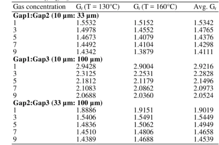
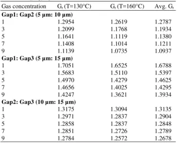
The input matching array consists of gaps conductance ratios as shown in Table 1 and 2 with noisy average conductance ratios shown in Table 3. As a ratio is a dimensionless number+, then conductance gap ratio should in theory be the same at all temperatures as shown in Eq. 1:

T T1 T T2 T T2

n n n

m m m

G G G

G = G = G =

     

≅

     

      (1)

Equation 1 assumes that all gaps are affected almost equally by temperature providing no phase transformation occurs within the used temperature range as it is the case shown in Table 1 and 2 for temperatures up to 160°C. This eliminates temperature as a variable of concern, when it comes to signal detection and gas discrimination and reduces significantly the number of necessary data inputs.

Fig. 2: Transient response for SAU

Fig. 3: Transient response for noisy SAU

Table 1: Average conductance ratios (Avg. Gr) for sensor unit arrays: X1, X2, X3

Gas concentration Gr (T = 130°C) Gr (T = 160°C) Avg. Gr

Gap1:Gap2 (10 µm: 33 µm)

1 1.5532 1.5152 1.5342

3 1.4978 1.4552 1.4765

5 1.4673 1.4079 1.4376

7 1.4492 1.4104 1.4298

9 1.4342 1.3879 1.4111

Gap1:Gap3 (10 µm: 100 µm)

1 2.9428 2.9004 2.9216

3 2.3125 2.2531 2.2828

5 2.1812 2.1179 2.1496

7 2.1083 2.0862 2.0973

9 2.0688 2.0360 2.0524

Gap2:Gap3 (33 µm: 100 µm)

1 1.8886 1.9151 1.9019

3 1.5406 1.5491 1.5449

5 1.4836 1.5062 1.4949

7 1.4510 1.4806 1.4658

(3)

429

Table 2: Average conductance ratios (Avg. Gr) for sensor unit arrays: X4, X5, X6

Gas concentration Gr (T=130°C) Gr (T=160°C) Avg. Gr

Gap1: Gap2 (5 µm: 10 µm)

1 1.2954 1.2619 1.2787

3 1.2099 1.1768 1.1934

5 1.1641 1.1119 1.1380

7 1.1408 1.1014 1.1211

9 1.1139 1.0735 1.0937

Gap1: Gap3 (5 µm: 15 µm)

1 1.7051 1.6525 1.6788

3 1.5683 1.5110 1.5397

5 1.4970 1.4279 1.4625

7 1.4656 1.4025 1.4295

9 1.4247 1.3621 1.3934

Gap2: Gap3 (10 µm: 15 µm)

1 1.3175 1.3094 1.3135

3 1.2971 1.2837 1.2904

5 1.2858 1.2837 1.2848

7 1.2851 1.2726 1.2789

9 1.2784 1.2572 1.2678

Table 3: Average conductance ratios for noisy SAU

Gas concentration Avg. Gr

X1, X2, X3 Gap1: Gap2 (10 µm: 33 µm)

1 0.192

3 0.187

5 0.183

7 0.181

9 0.179

X4 X5, X6Gap1:Gap3 (5 µm: 15 µm)

1 0.406

3 0.378

5 0.364

7 0.357

9 0.349

RESULTS

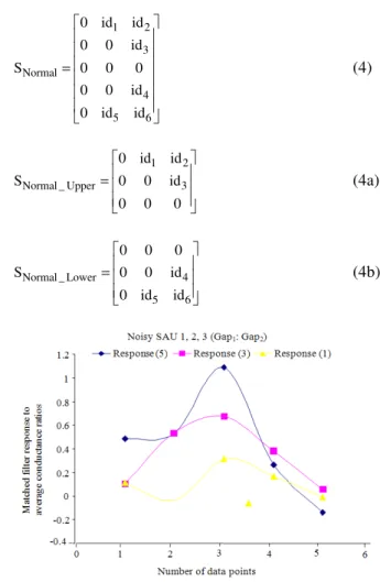
The following matrices show the response of the 5-3-1 rule based matched filter with intelligent identifiers at the top and bottom corners to the average conductance of six array units with and without noise.

2.380 0.103 0.109

4.296 4.357 -0.031

10.611 4.461 2.235

4.034 4.198 0.166

1.758 0.052 0.009

 

 

 ₋ 

 

MF: Sensors (1, 2, 3): gap1:gap2

0.481 0.103 0.109

0.529 0.533 -0.031

1.093 0.672 0.315

0.267 0.377 0.166

-0.142 0.052 -0.009

 

 

 

MF: Sensors (1, 2, 3) gap1:gap2 (Noisy)

6.078 0.243 0.224

11.246 12.837 -0.104

31.125 12.678 6.955

10.765 12.323 0.321

5.007 0.061 -0.044

 

 

 

MF: Sensors (1, 2, 3) gap1:gap3

     

 

     

 

0.022 -0.045 2.141

0.208 5.536

4.864

3.170 5.839

13.982

0.060 -5.786 5.187

0.144 0.152

2.861

1.510 0.089 0.090

2.663 2.735 -0.030

6.606 2.814 1.423

2.448 2.602 0.135

1.016 0.038 -0.010

 

 

 

2.372 0.116 0.116

4.278 4.436 -0.041

10.759 4.515 2.306

4.002 4.257 0.174

1.743 0.048 -0.015

 

 

 

0.750 0.116 0.116

1.065 1.099 -0.041

2.486 1.220 0.608

0.789 0.935 0.174

0.121 0.048 -0.015

 

 

 

MF: Sensors (4, 5, 6): gap1:gap3 (noisy)

1.790 0.083 0.090

3.202 3.219 -0.021

7.84 13.347 1.659

2.983 3.087 0.138

1.255 0.046 -0.003

 

 

 

DISCUSSION

(4)

signal to the MF. Figure 6 illustrates effect of gap width on SAU conductance and in turn the response of the MF to the output signals from the sensors.

The developed 5-3-1 algorithm provides intelligent identifiers per matched filter response with symmetrical data difference array, which reduces the amount of processed data and achieve excellent identification. The 5-3-1 algorithm is as follows:

• The detected sensor array unit signals are processed and stored into data matrices, each matrix has six identifiers at upper and lower corners as shown in Eq. 2:

11 1 2

21 22 3

31 32 33

41 42 4

51 5 6

a id id

a a id

S a a a

a a id

a id id

 

 

=_ _

 

 

(2)

• Using tagged identifiers, the detected signals are identified then compared with reference ones and the result is stored in a new matrix as in Eq. 3:

11 11

21 21 22 22

identified 31 31 32 32 33 33

41 41 42 42

51 51

a b 0 0

a b a b 0

S a b a b a b

a b a b 0

a b 0 0

−

 

 

− −

 

=_ − − − _

− −

 

 ₋ 

 

(3)

• The identifiers are reinstated and data is rounded up in the new matrix to the nearest integer

• The resulting matrix is Folded and respective data values are compared, knowing that:

11 11 51 51

(a −b )=(a −b )

21 21 41 41

(a −b )=(a −b )

22 22 42 42

(a −b )=(a −b )

Fig. 4: MF response to SAU normal signals

The symmetry of the matrix allows us to use either half for identification and decision making. If the received signals are noisy, the output array would have large but decrementing data values; otherwise it will contain only zeros. Hence two cases are possible: Normal signal:

1 2

3

Normal

4

5 6

0 id id 0 0 id

S 0 0 0

0 0 id 0 id id

 

 

=_ _

 

 

(4)

1 2

Normal _ Upper 3

0 id id

S 0 0 id

0 0 0

 

 

=_ _

 

 

(4a)

Normal _ Lower 4

5 6

0 0 0

S 0 0 id

0 id id

 

 

= 

 

 

(4b)

Fig. 5: MF response to SAU noisy signals

(5)

431 Noisy signal:

1 2

3

Noisy 31 31 32 32 33 33

4

5 6

0 id id

0 0 id

S a b a b a b

0 0 id

0 id id

        = − − −         (5) 1 2

Noisy _ Upper 3

31 31 32 32 33 33

0 id id

S 0 0 id

a b a b a b

    =   ₋ ₋ ₋    (5a)

31 31 32 32 33 33

Noisy _ Lower 4

5 6

a b a b a b

S 0 0 id

0 id id

− − −     =      (5b)

Data identifiers are rearranged to produce a 3by 3 matrix:

1 2 3

Final 1 2 3

6 5 4

id id id

S D D D

id id id

    =      (6)

where, D1 D2 D3 are interlarded as follows:

31 31 1 32 32

2 33 33 3

(a b ) D 2.5 (a b ) D 5 (a b ) D

− = = −

= = − = (7)

Hence:

1 2 3

1 1

Final _ Noisy 1

6 5 4

id id id

D D

S D

2.5 5 id id id

      =_ _     (8)

1 2 3

Final _ Normal

6 5 4

id id id

S 0 0 0

id id id

    =      (9)

Now as the identifiers are unique for each sensor array unit and there is a relationship between data values (D1, D2, D3), then the final output can be sorted in any of the line arrays as follows as each one is unique to the sensor array unit and provides valuable indication to the quality of data obtained, with preference to line array A as it has maximum data value. Also, each line array has two guarding identifiers to mark start and stop of data values:

Final _ NoisyA 1 1 6

S =_id D id _ (10a)

1

Final _ NoisyB 2 5

D

S id id

2.5

 

= 

  (10b)

1

Final _ NoisyC 3 4

D

S id id

5

 

= 

  (10c)

Applying the previous to prove validity to SAU (1, 2, 3) Gap1: Gap2, we obtain:

From Eq. 3:

1.899 0.000 0.00

3.767 3.824 0.00

9.518 3.789 1.92

3.767 3.821 0.00

1.900 0.000 0.00

               

From Eq. 5:

1.9 0.103 0.109

3.8 3.8 -0.031

9.5 3.8 1.900

3.8 3.8 0.166

1.9 0.052 -0.009

               

From Eq. 6-8:

0 0.103 0.109

0 0.000 -0.031

10 4.000 2.000

0 0.000 0.166

0 0.052 -0.009

               

From (10a), (10b) and (10c):

0.103 0.109 -0.031

10 4.000 2.000

0.052 -0.009 0.166

 

 

 

The final intelligently guarded sequences that are used for identification and signal testing of an SAU are given by:

[

]

Final _ NoisyA

S = 0.103 10 0.052

[

]

Final _ NoisyB

S = 0.109 4 −0.009

[

]

Final _ NoisyC

S = −0.031 2 0.166

CONCLUSION

(6)

algorithm involves deduction from presented data whether the target data is valid or not. The designed and tested algorithm proved its validity with the novel feature of intelligent identifiers that regardless of the noise corrupting or interfering with the signal can identify the source and recalls the correct. The tested SAU devices proved to be stable over temperature variations for the detection of acceptor gases such as NO2 with inter-electrode gap separation per fixed deposited film thickness playing an important role in conductivity level per applied gas concentration. For a fixed gap, it is shown that device conductance increased as the gas concentration increased.

REFERENCES

Abella, M., J.J. Vaquero, M.L. Soto-Montenegro, E. Lage and M. Desco, 2009. Sinogram bow-tie filtering in FBP PET reconstruction. Med. Phys., 36: 1663-1670. DOI: 10.1118/1.3096707

Bocchi, L., G. Coppini, J. Nori and G. Valli, 2004. Detection of single and clustered microcalcifications in mammograms using fractals models and neural networks. Med. Eng. Phys.,

26: 303-312. DOI:

10.1016/j.medengphy.2003.11.009

Chen, J.Y., X.P. Zhong and X.Z. Feng, 2006. A template matching method of wideband sonar detection. J. Phys. Conf. Ser., 48: 54-58. DOI: 10.1088/1742-6596/48/1/010

Chen, X., Z. Xu, T. Chen, J. Wang and L. Li, 2009. Detecting pills in fabric images based on

multi-scale matched filtering. Textile Res. J., 79: 1389-1395.

DOI: 10.1177/0040517508099913

Dorronsoro, J.R., V. Lopez, C.S. Cruz and J.A. Siguenza, 2003. Autoassociative neural networks and noise filtering. IEEE Trans. Signal Proc., 51: 1431-1438. DOI: 10.1109/TSP.2003.810276

Fan, L., E. Boni, P. Tortoli and D.H. Evans, 2004. Multigate transcranial Doppler ultrasound system with real-time embolic signal identification and archival. IEEE Trans. Ultrason. Ferroelect.

Control, 53: 1053-1061. DOI:

10.1109/TUFFC.2006.117

Imam, N. and J. Barhen, 2009. Acoustic source localization via time difference of arrival estimation for distributed sensor networks using tera-scale optical core devices. J. Sensors, 2009: 1-11. DOI: 10.1155/2009/187916

Khairnar, D.G., S.N. Merchant and U.B. Desai, 2008. Radar signal detection in non-Gaussian noise using RBF Neural Network. J. Comput., 3: 32-39. DOI: 10.4304/jcp.3.1.32-39

Knipp, D., R.A. Street, H. Stiebig, M. Krause and J.P. Lu et al., 2006. Color aliasing free thin-film sensor array. Sensors Actuat., 128: 333-338. DOI: 10.1016/j.sna.2006.02.007

Mohamed, S., H.A. Maan, M. Shaker and T.A. Salih, 2008. Design and implementation of a dynamic analog matched filter using FPAA technology. Proceeding of the World Congress On Science, Engineering and Technology, Dec. 17-19, World Academy of Science, Engineering and Technology, Bangkok, Thailand, pp: 206-210. http://www.waset.org/journals/waset/v48/v48-33.pdf

Pados, D.A., 2001. An iterative algorithm for the computation of the MVDR filter. IEEE Trans.

Signal Proc., 49: 290-300.

http://www.telecom.tuc.gr/~karystinos/study_TSP. pdf

Ricci, S., A. Dallai, E. Boni, L. Bassi and F. Guidi et al., 2008. Embedded system for real-time digital processing of medical ultrasound Doppler signals. EURASIP J. Adv. Signal Proc., 418235: 1-7. DOI: 10.1155/2008/418235

Sheriff, S.D., 2010. Matched filter separation of magnetic anomalies caused by scattered surface debris at archaeological sites. Near Surface Geophys., 8: 145-150. DOI: 10.3997/1873-0604.2009057

Shi, S., Y. Shang and Q. Liang, 2007. A novel linear beamforming algorithm. Piers Online, 3: 1089-1092. DOI: 0.2529/PIERS061007112619

Soaresa, C. and S.R.M. Jesusb, 2003. Broadband matched-field processing: Coherent and incoherent approaches. J. Acoust. Soc. Am., 113: 2587-2598. DOI: 10.1121/1.1564016

Tandra, R. and A. Sahai, 2008. SNR walls for signal

detection. IEEE J. Select. Topics Signal Proc., 2: 4-17.

DOI: 10.1109/JSTSP.2007.914879

Zeng, Y., Y.C. Liang, A.T. Hoang and R. Zhang, 2010. A review on spectrum sensing for cognitive radio: Challenges and solutions. EURASIP J. Adv. Signal Proc., 381465: 1-15. DOI: 10.1155/2010/381465 Zurk, L.M., B.N. Lee and J. Ward, 2003. Source motion