ABSTRACT: The design of a passive fault-tolerant control for an underactuated re-entry capsule is considered in this paper; however, the control input of the capsule is failed. At irst, kinematics and dynamics of the capsule are studied and modeled, and adaptive control law is used to design a passive controller for the control of the capsule. The guidance law for the capsule is designed based on the guidance law which is used in Apollo. A simulation is performed based on Apollo capsule in order to assess the controller. The result shows good control authority of the controller in the presence of failure in roll and yaw control channels. It is also shown that the guidance law is not credible in the presence of yaw channel input failure.
KEYWORDS: Passive, Fault-tolerant control, Underactuated, Re-entry capsule, 6 DOF modeling.
Passive Fault-Tolerant Control of an
Underactuated Re-Entry Capsule
Alireza Alikhani1
INTRODUCTION
Today, modern systems based on advanced control ones can be developed to achieve high performance and safety. Design of conventional closed-loop control for complex systems may not have a satisfactory answer or can even cause system instability when error and failures of actuators, sensors or other components of the control system occurred. To overcome these problems and weaknesses, new control systems have been developed to confront and redress system downtime as well as to ensure eiciency and stability. his problem is founded on much higher importance for safety-critical systems such as an aircrat, spacecrat, chemical plants, nuclear power plants, and systems. In such systems, the slightest error can cause accidents and catastrophes load. Hence, the demand and need for increased reliability, safety, and compensation for error are very high, and the designed control system must be able to handle possible errors in these types of systems in order to improve reliability and accessibility. This type of control system is known as fault-tolerant control systems (FTCS). In other words, FTCS have the ability to automatically modify and adapt the defective components. In addition, the overall behaviour of the system in terms of stability and performance is maintained at acceptable levels. Since the law in each control loop components (actuators, sensors, and plant) cannot be ignored, FTCS are one of the active branches in the ield of industrial control.
In the design of the controller for dynamic systems, it is assumed that, in the occurrence of failure in the actuators, the system remains fully-actuated. However, there is a condition in which the system is underactuated: the number of independent inputs is less than the number of system’s degrees of freedom
1.Ministry of Science, Research and Technology – Aerospace Research Institute – Astronautics Department – Islamic Republic of Iran.
Author for correspondence: Alireza Alikhani – Ministry of Science, Research and Technology – Aerospace Research Institute – Astronautics Department | PO box 14665-834 – Tehran – Islamic Republic of Iran | Email: [email protected]
(DoF). hese systems are complicated, and commonly con- trol methods are not usable for compensation. So the control of these systems is seriously faced with critical challenges (Crouch 1984).
In this paper, the control problem of the underactuated spacecrat in the atmospheric reentry phase is studied. It is aimed to study the fault-tolerant control problem of spacecrat attitude control in the re-entry phase.
Commonly, FTCS are summarized into 2 categories: passive (PFTCS) and active (AFTCS) (Jiang and Yu 2012). In PFTCS, controllers are designed to be robust against a class of presumed faults and so they have a ixed structure. his approach does not need FDD subsystem and does not have controller reconiguration. A list of potential defects likely already prepared at the design stage as well as failure modes and normal operating conditions are considered in the design phase of this approach. In other words, the passive controller is a controller with a fixed structure, so it can be used for limited situations. In AFTCS, the system component failures are actively controlled by reconiguring control actions so that the stability and acceptable performance of the entire system can be maintained. herefore, the main purpose of a FTCS is to design a controller to ensure stability and performance in a good level. his ability exists not only when all control subsystems are in healthy situation, but also in cases when there are failures in control system components (sensors, actuators, etc.).
Statistical studies have shown that about 24% of crashes in military and civilian spacecrat attitude control systems have been related to thruster defects (Tafazoli 2009). In the literature, a survey of fault-tolerant control of the spacecrat has founded numerous papers in orbital motion phase, but there is no report for the re-entry one. Next, there is a review of some of them.
An underactuated spacecraft was stabilized by using 2 momentum wheel actuators (Krishnan et al. 1995), and a proposed control law reduced the control efort required for a non-smooth time invariant feedback control of an under- actuated spacecrat (Tsiotras and Luo 1997).
In another study, it was found a sliding mode control designed for stabilization of the angular velocity of a rigid body. he system is supposed to have only 2 control torques and to be subjected to external disturbances (Floquet et al. 2000). In Eshaghi and Wang (2001), Lyapunov direct method was used to control and stabilize a rigid satellite, and one of the input channels has lost their control. his method does not need to identify the failure and switching to the new control law. Morin
(1996) showed that most proposed controls in the past are not robust to errors in actuators’ location. his author proposed a robust asymptotically-stabilizing feedback control law.
An adaptive asymptotic stabilization of angular velocities of a rigid body with 2 control inputs in the presence of uncertainty in dynamic parameters was presented in Wang and Tao (2007). Hamiltonian control approach for the stabilization of a rigid body system that is controlled by 2 torques was presented by Aguilar-Ibanez et al. (2008). In this stabilization, the closed-loop system was forced to be globally asymptotically-stable by solving a feasible matching condition.
In Zheng and Ge (2008), a backstepping control method was used to stabilize an underactuated spacecrat which has only 2 control inputs. In Bajodah (2009), it was presented a novel concept of feedback linearization which is introduced for smooth asymptotic stabilization of underactuated spacecrat equipped with 1 or 2 degrees of actuation, and the concept is based on generalized inversion.
In the study of Pong (2009), a Model Predictive Control (MPC) was proposed as a control technique to solve thruster failure recovery. A method of online MPC was described, implemented, and tested on the Experimental Satellites (SPHERES) testbed at the Massachusetts Institute of Technology (MIT) and on the International Space Station (ISS). hese results show that the proposed control improved the performance of underactuated spacecrat. Jin and Xu (2010) presented the angular velocity stabilization and attitude stabilization control for an underactuated spacecrat by using 2 single gimbal control moment gyros (SGCMGs) as actuators. In Wang et al. (2013), suicient and necessary condition of controllability of underactuated spacecrat was illustrated on the basis of Lie Algebra Rank Condition (LARC).
In Mirshams et al. (2014), angular and 3-axis stabilization control laws were designed for the case of 2 existing thrusters by Lyapunov method and LaSalle invariant theorem. Sliding mode control was used for passive fault-tolerant control of a lexible spacecrat with faulty thrusters. Tube-based MPC approach was used in attitude control of an underactuated spacecrat by Mirshams and Khosrojerdi (2016).
“Simulation” and, i nally, conclusions and recommendations are presented.
MODELLING OF THE RE-ENTRY CAPSULE
Kinematics and dynamics of the re-entry capsule are studied in this section, and the relative equations are derived.
KINEMATICS
SBE is the position vector representing the center of body coordinate with respect to the Earth center Earth i xed (ECEF) coordinate system. h e velocity vector is derived by dif erentiating the position vector:
h e expression of Eq. 2 is carried out in the geographic coordinate, so it can be shown as follows:
where DEis the derivative operator and v E B
is the velocity
of the body coordinate, both in relation to the ECEF coordinate system.
By using the well-known operator equation acting on the position vector, Eq. 1 is rewritten as:
where DG is the derivative operator in the geographic
coordi-nate (G), i.e. the origin at the center of mass of the spacecrat , x-axis toward the North Pole, y-axis toward the east, and z-axis toward the Earth’s center (Fig. 1); ωGE is the angular velocity
of the geographic coordinate relative to the ECEF coordinate system.
Figure 1. Geographic coordinate system with its vectors g1, g2, and g3.
Gre enw ich
M erid
ian
Equat
or
g1
g2
g3
h
ϕ
λ
h e position of the capsule in the geographic coordinate can be dei ned as follows:
R is dei ned as:
where h represents the distance of the capsule from the Earth; Re is the Earth’s radius, thus:
h e velocity of the capsule with respect to ECEF in the wind coordinate system, i.e. a coordinate system which is dei ned in relation to the crat ’s velocity V, is:
where W is the wind coordinate.
Using a transformation matrix, Eq. 7 can be expressed in the geographic coordinate as:
where TG
W is the transformation matrix from wind to Geographic
coordinate.
h e angular velocity of the geographic coordinate with respect to ECEF can be represented by:
where λ and l are latitude and longitude of the capsule position, respectively; {y2}E is the second unit vector of ECEF
coordinate; {x3}l is the third unit vector of the Earth’s center
inertial (ECI) coordinate. (1)
(3)
(4)
(5)
(6)
(7)
(8)
h e angular velocity can be expressed in the geographic coordinate by transformation matrixes:
In addition:
where T G E and T
G
l are transformation matrixes from ECEF and
ECI to the geographic coordinate, respectively.
By substituting Eqs. 6 – 10 in Eq. 3, the following relation can be derived for kinematics of the re-entry capsule:
where: {g3}G is the third unit vector of the geographic coordinate.
TRANSLATIONAL MOTION DYNAMICS
From the Newton’s second law, one has:
where aB I is the acceleration and m
B is mass of body
h e acceleration of the capsule is derived by the second derivative of the position:
where SBI represents the position of the center in body coordinate system with respect to the ECI coordinate:
where SEI is the position of the center in ECEF coordinate system with respect to the ECI coordinate system. Since the centers of ECEF and ECI are coincident, one has:
By substituting Eq. 15 in Eq. 13, and using vector derivative rules,
h us, the derivative is 0:
Equation 17 can be rewritten as:
On the other hand, the summation of external exerted forces is:
where: f
a, fg, and fu are aerodynamic force, gravity force, and
motor force, respectively. In this modelling, f
u is considering
to be 0.
The aerodynamic forces are commonly resolved into 2 components: drag (D) is the force component parallel to the direction of the relative motion, and lit (L) is the force component perpendicular to the direction of the relative motion. h en, these forces in the wind coordinate system are calculated according to Roskam (2001):
where q – = 1/2ρv2, C
D = CD0 + CDαα and CL = CL0 + CLαα.
The gravity force in the geographic coordinate can be calculated by:
(10)
(18)
(19)
(20)
(21)
(22)
(23)
(24)
(25) angular velocity of earth = constant
(11)
(12)
(13)
(14)
(15)
(16)
(17)
h e i rst term of Eq. 25 can be written as: where ωBI is the angular velocity of the body coordinate with
respect to the inertial coordinate:
h us, Eq. 25 can be rewritten as follows:
h e above equation can be explained in the wind coordinate system:
where and and the angular velocity
of wind coordinate with respect to ECEF is dei ned as:
where ø is the roll angle; γ is the path angle; ξ is the heading angle; w
1 is the i rst unit vector of the wind coordinate system; v
2 is the second unit vector of the velocity coordinate sys-tem; z
3 is the third unit vector of the body coordinate system. By substituting Eq. 29 in Eq. 28, the translational dynamic equation of the re-entry capsule can be expressed as follows:
So Eq. 32 is rewritten as follows:
By substituting Eq. 34 in Eq. 31:
h is equation can be explained in the body coordinate:
h e angular velocity of the geographic coordinate with respect to the inertial coordinate is obtained as follows:
And M is the summation of external exerted moments:
where M
a is the aerodynamic moment; Mu is the control moment.
h e aerodynamic moments for pitch, roll, and yaw channels are calculated by (Roskam 2001):
where Cl, Cm and Cn are roll and pitch, and yaw moment coefficients, respectively, which can be calculated by the following formulas:
(26)
(27)
(28)
(29)
(30)
(31)
(32) where and and the angular velocity where and and the angular velocity
ROTATIONAL MOTION DYNAMICS
Euler’s law is expressed as follows:
IB BI is the angular momentum so the i rst term of Eq. 31 is:
(33)
(34)
(35)
(36)
(37)
(38)
(39)
(40)
GUIDANCE LAW OF THE RE-ENTRY
A GNC system is formed by 3 main subsystems: guidance, navigation, and control. h e task of the navigation is to process the sensor outputs and produce an estimation of the attitude and position of the spacecrat . Guidance and control functions work in parallel. h e guidance unit at er receiving an estimated value of attitude and position from the navigation one will produce reference signals for the control unit, which must trace the guidance signals.
One of the common shapes for re-entry vehicles is the blunt bodies (similar to the Apollo spacecraft). This configuration has small and nearly constant lift-to-drag ratio (L/D) and can be considered and designed to fly at a constant angle of attack.
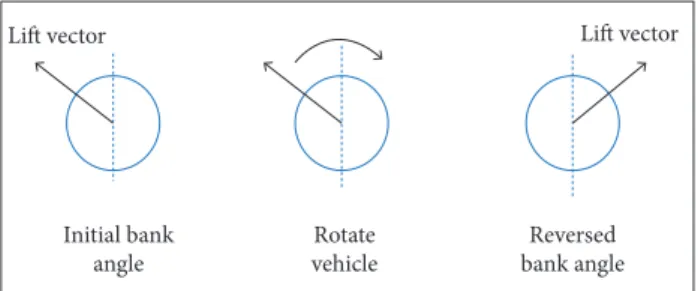
In these vehicles, the tracking of the trajectories has been controlled by modulation of the bank angle. Altitude and direction of the vehicle are controlled by the bank angle magnitude and sign, respectively. A conceptual schematics of this method is illustrated in Fig. 2. Modulation of bank angle, energy, and range for the target of the vehicle are managed in order to achieve the precise landing.
of bank angle modulation to manage energy and range for the target, rigorously tested, verii ed, and l own.
In the re-entry of the capsule, the target point is the recovery position where parachute must be opened. Its guidance scheme is divided into dif erent phases, which are selected depending on the current state of the vehicle (Guerreiro 2011):
• Initial Roll.
• Constant Drag (optional).
• Up Control + Ballistic (optional).
• Targeting.
The first phase of the guidance scheme is the Initial Roll. In this phase, the lift vector is rotated downwards by banking the capsule for 180 degrees in order to maximize the force that pulls down the vehicle and ensures that it is captured. This phase lasts until a maximum altitude rate is reached, at a point where a significant amount of energy has been dissipated in order to avoid skipping, while enough energy remains so that the vehicle is still able to reach the final target.
The following optional phases — Constant Drag, Up Control, and Ballistic — allow the additional dissipation of energy and correction of the range until the predicted miss (that is, the distance between the landing site and the predicted landing point) is less than a pre-specific value. These are only used to adjust the vehicle’s position and energy to the values required for the trigger of the targeting phase. In the Constant Drag phase, a constant drag value is tracked. The Up Control and Ballistic phases allow performing a skip-entry, where the Reentry Vehicle is controlled in an upward trajectory and projected out of the atmosphere with a certain velocity as well as flight path angle. The Ballistic phase is activated until the RV returns again to the atmospheric environment, expectedly at a satisfactory range from the target.
When the RV is at approximately the desired range from the target and has an acceptable energy level, the Targeting phase is activated. In this final phase, the RV aims at the targeting position. It is done by tracking a reference trajectory generated online, using a gain-scheduled PID controller whose gains are the derivatives of range with respect to altitude rate F2 (V), drag F1 (V), and L/DF3 (V), also stored on-board. The expression used to predict the range in this final phase is (Guerreiro 2011):
Figure 2. Bank angle modulation.
Lift vector Lift vector
Reversed bank angle Rotate
vehicle Initial bank
angle
(41)
A re-entry guidance algorithm must be consisted of (Bairstow 2006):
• Capture into the atmosphere.
• Manage energy by removing excess of velocity through drag management.
• Steer to a target.
In this paper, the algorithm will be based on the Apollo re-entry guidance algorithm, in which it is used the principle
where S is the range; h represents altitude; D is the drag; the subscripts “pred” and “ref ” stand for “predicted” and “reference”. Note that the reference values are all taken from the entry proi le stored on-board and are mapped with respect to the velocity V. h e predicted range thus computed is plugged into the computation of the desired L/D ratio (Guerreiro 2011):
robust controls; model predictive control; variable structure and sliding mode control; linear quadratic; pseudo-inverse/ control mixer; gain scheduling/linear parameter varying; feedback linearization or dynamic inversion; generalized internal model control; (model reference) adaptive control/ model following; eigenstructure assignment; multiple-model; intelligent control using expert systems, neural networks, fuzzy logic, and learning methodologies. Four main criteria are used for classification of these methods: (1) mathematical design tools; (2) design approaches; (3) reconfiguration mechanisms; and (4) type of systems to be dealt with.
Selecting the appropriate method among the proposed ones depends on the error compensation methods in the presence of failures in real time. For this purpose, a new control structure configuration must be proactive in terms of bondage with the least try and error and the selected method as tangible even if the answer is not optimized.
One of the proposed methods is the adaptive control, which is robust to dynamic models and parameter uncertainties. This method, according to the classification, is considered as PFTCS. In order to control the defective dynamic system, there is no need for the FDD module, but it has a small working range and cannot cover any type of crashes. The important fact about this method is that, despite the changes in the parameters of the dynamic coefficients, the presence of update law for control coefficients ensures the pursuit of sustainability and tracking guidance law, so spacecraft can continue the mission. Therefore, it can be anticipated that, in this method, there is no fault detector unit, but it has a good robustness against the malfunctioning of the actuators.
h e revision and selection of other methods of passive and active fault-tolerant control are presented next. In this paper, Model Reference Adaptive Control (MRAC, also known as Model Reference Adaptive System — MRAS) is considered. h is approach is one of the adaptive control methods. h e general concept behind MRAC is to construct a closed-loop dynamic system with updatable parameters that change the system’s response. h e response of the actual system is compared with a response of the reference model.
h e control parameters are updated according to an adaptive law based on these errors. h e purpose of the adaptive law is: the undei ned parameters should converge to values that make the dynamic system reaction match the response of the reference model.
In the Apollo guidance scheme, the Lateral Logic function is called to ensure the lateral guidance control in all phases. h e lateral control is performed by reacting the horizontal component of L about the vertical axis, either to the right or to the let , which therefore takes the RV into any of the 2 directions via determination of a bank angle control command. h is is done by the expression (Guerreiro 2011):
where K1 and K2 are indicators for switching the bank angle sign; L/Dmax is the maximum lit -to-drag ratio.
Note that this maximum value is a constant and that the argument of the arccos function comes from the result of Eq. 43 in the i nal phase of the entry guidance algorithm. h e orientation of the lit reaction, that is, the values of K1 and K2, is determined based on the predicted cross range miss: if it exceeds a predetermined fraction of the vehicle cross range capability, the direction of the lit vector is changed.
PASSIVE FAULT-TOLERANT
CONTROL DESIGN
Due to real-time requirements and the nature of the dynamics of the system, there is usually a very limited amount of time available to carry out the post-fault model construction and control reconfiguration actions. The trade-off between various design objectives and the interaction between different subsystems have to be carried out online in real time. However, for AFTCS, there are several additional challenges besides those in the conventional control systems, such as redundancy management, integration of FDD and reconfigurable controller, safety and reliability design purposes. The existing fault-tolerant control methods are categorized into one of the following manners: H∞ and other (43)
(44)
σ
c=
K
2arccos (
L/D
/
L/D
max) + 2π
K
1For the design of the MRAC controller, the following steps must be taken (Astrom and Wittenmark 1994):
1. Determine the structure of the controller.
2. Get the error equation.
3. Select an appropriate Lyapunov function that tend the error to 0 and provide update law for parameters. h e dynamic model of the system is as follows:
By substituting Eq. 54 in Eq. 53, one has:
where � is the system matrix, b is the input matrix and u is the input vector.
And the reference model is considered as:
Now, the Lyapunov candidate is selected as follows:
where L is the adaptive law gain that must be selected. If parameters are tending to their ideal values and error becomes 0, then Lyapunov function becomes 0. By time derivative of V, there are:
By choosing the adaptive law, one has:
h e time derivative of the Lyapunov candidate function V
becomes negative dei nite:
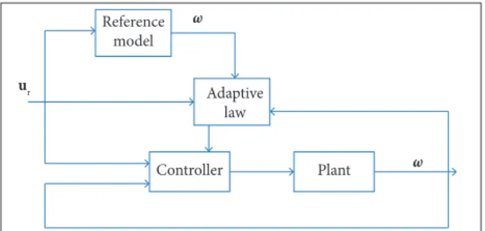
Figure 3 shows the block diagram of the designed controller. (45)
(46)
(47)
(48)
(51)
(52)
(53)
(54) (49)
(50) where am and bm are the coei cient of the reference model.
h e dynamic error and controll er structure are determined by the following equations (Astrom and Wittenmark 1994):
where Ѳ
1 and Ѳ2 are gain controller; ur is the reference signal.
h e goal of the controller is to track the reference signal, then:
h e ideal value of gains is obtained as:
and, in order to minimize the error, using error equation, there are:
h e error between the ideal and estimated gains is introduced as follows:
(55)
(56)
(57)
(58)
(59)
(60)
(61)
Reference model
Adaptive law
Controller Plant
u r
ω
ω
Figure 3. Block diagram of the designed controller.
SIMULATION
Table 3. Stability derivatives parameters of the simulated spacecraft.
Parameter Mean value
Cl
β −3
Cmα −0.01
Cn
β ≈ 0
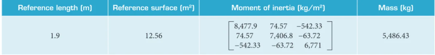
to carry out a simulation, relevant information of this spacecrat is used, and some of its mass-volumetric features have been used in the simulation shown in Table 1.
Figure 4. Re-entry module of Apollo.
In order to simulate and illustrate the operation of the controller, various scenarios will be considered to represent the behavior of the closed-loop system in the state of being healthy and in the malfunctioning of the actuators. These scenarios are in accordance with Table 2.
h e initial conditions for the simulation are considered as:
Mode Simulation scenarios Failure modes
1 All actuators are healthy ��, ��, �� ≠ 0
2 Roll channel input failed ��, �� ≠ 0; �� = 0
3 Pitch channel input failed ��, �� ≠ 0; �� = 0
4 Yaw channel input failed ��, �� ≠ 0; �� = 0
Table 1. Mass-volumetric features of Apollo.
Reference length (m) Reference surface (m2) Moment of inertia (kg/m2) Mass (kg)
1.9 12.56
8,477.9 74.57 −542.33 74.57 7,406.8 −63.72 −542.33 −63.72 6,771
5,486.43
Source: Guerreiro (2011).
Table 2. Simulation scenarios.
have been brought up together to be easily compared with each other. As can be observed, the lack of control forces on the pitch or roll channels does not affect the actual path, and the bank angle is satisfied by the other control input. Therefore, the pursuit of latitude and longitude coordinates of the path does not change. However, with the failure on the yaw channel actuators, the ability to prosecute the guidance law is lost and caused deviation from the desired path.
In order to analyze the results, the equation of spacecrat re-entry mechanism is determined. Assuming that the cross momentum of inertia is 0, Euler equation (Eq. 36) can be written as:
where mc
i is the control input; m A
i is aerodynamic moment for
each channel.
According to Eqs. 39 and 41, as well as Table 3, Eq. 62 is rewritten as:
(62) h e i nal conditions of the simulation are:
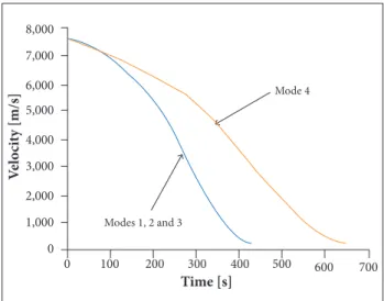
The final condition is based on bucket energy. The values of the parameter of the stability derivatives as well as the parameters of Table 3. Now, according to the tables values, the simulation of the designed control and guidance law is done, and the results are shown in Figs. 5 to 7). The results
λ = 0o l = 0o
Match number ≅ 0.8
h = 88600 m
λ = 0o l = –16.48o ν = 7620 m/s
Figure 7. Velocity diagram of the spacecraft for scenarios 1, 2, 3, and 4.
As it is seen, in the yaw channel, C
nβ is very low and β (side
slip angle) is trimmed to 0, so the aerodynamic moment does not have any ef ect, and then the failure of actuators in this channel has most ef ort on attitude control of the spacecrat . However, if the actuators of roll and pitch channels are corrupted, the aerodynamic moment is still exerted. Besides, according to dependency of aerodynamic moment to α and
β angles, as well as coupling of angles, the bank angle can be controlled by roll and yaw channels separately.
Simulation results confirm this subject, and the important point of this simulation is: the adaptive control method has this ability in such a way that the actuators’ failure, considered as the uncertainty in the input control and other healthy inputs, helps to compensate the existing failure.
0 .3
Modes 1, 2 and 3
Mode 4 0.25
0.2
0.15
0.1
0.05
0
–0.05
–20 –15 –10 –5 0 5 10
L
a
ti
t
u
d
e
Longitude
8,000
Modes 1, 2 and 3
Mode 4 7,000
6,000
5,000
4,000
3,000
2,000
1,000
0
0 100 200 300 400 500 600 700
V
el
o
ci
ty [m/s]
Time [s]
250
Modes 1, 2 and 3
Mode 4 200
150
100
50
0
–50
–100
0 100 200 300 400 500 600 700
ϕ
[d
eg
]
Time [s]
Figure 5. Actual paths tracked by the spacecraft for scenarios 1, 2, 3, and 4.
Figure 6. Actual bank angle of the spacecraft for scenarios 1, 2, 3, and 4.
(63)
CONCLUSION
REFERENCES
Aguilar-Ibanez C, Suarez-Castanon MS, Guzman-Aguilar F (2008) Stabilization of the angular velocity of a rigid body system torques: energy matching condition. Proceedings of the American Control Conference; Seattle, USA.
Astrom K, Wittenmark B (1994) Adaptive control. 2nd Edition. Mineola: Dover Publication.
Bairstow HS (2006) Reentry guidance with extended range capability for low L/D spacecraft (Master’s thesis). Cambridge: Massachusetts Institute of Technology.
Bajodah AH (2009) Asymptotic perturbed feedback linearization of underactuated Euler’s dynamics. Int J Contr 82(10):1856-1869. doi: 10.1080/00207170902788613
Crouch PE (1984) Spacecraft attitude control and stabilization: applications of geometric control theory to rigid body models. IEEE Trans Automat Contr 29(4):321-331. doi: 10.1109/TAC.1984.1103519
Eshaghi R, Wang F (2001) A Lyapunov-based failsafe controller for an underactuated rigid-body spacecraft. Proceedings of the AIAA Guidance, Navigation and Control Conference and Exhibit; Montreal, Canada.
Floquet T, Perruquetti W, Barbot JP (2000) Angular velocity stabilization of a rigid body via VSS control. J Dyn Sys Meas Control 122(4):669-673. doi: 10.1115/1.1316787
Guerreiro L (2011) Development of a guidance and control design tool for entry space vehicles with different lift-over-drag ratios (Master’s thesis). Lisbon: Technical University of Lisbon.
Jiang J, Yu X (2012) Fault-tolerant control systems: a comparative study between active and passive approaches. Annu Rev Contr 36(1):60-72. doi: 10.1016/j.arcontrol.2012.03.005
Jin L, Xu S (2010) Underactuated spacecraft angular velocity stabilization and three-axis attitude stabilization using two single gimbal control moment gyros. Acta Mech Sin 26(2):279-288. doi: 10.1007/ s10409-009-0272-4
Krishnan H, McClamroch NH, Reyhanoglum M (1995) Attitude
stabilization of a rigid spacecraft using two momentum wheel actuators. J Guid Contr Dynam 18(2):256-263. doi: 10.2514/3.21378
Mirshams M, Khosrojerdi M (2016) Attitude control of an underactuated spacecraft using tube-based MPC approach. Aero Sci Tech 48:140-145. doi: 10.1016/j.ast.2015.09.018
Mirshams M, Khosrojerdi M, Hasani M (2014) Passive fault-tolerant sliding mode attitude control for lexible spacecraft with faulty thrusters. Proc IME G J Aero Eng 228(12):2343-2357. doi: 10.1177/0954410013517671
Morin P (1996) Robust stabilization of the angular velocity of a rigid body with two controls. Eur J Contr 2(1):51-56. doi: 10.1016/S0947-3580(96)70028-6
Pong CM (2009) Autonomous thruster failer recovery for underactuated spacecraft (Master’s thesis). Cambridge: Massachusetts Institute of Technology.
Roskam J (2001) Airplane light dynamic and automatic light controls. Lawrence: DAR Corporation.
Tafazoli M (2009) A study of on-orbit spacecraft failures. Acta Astronau- tica 64(2-3):195-205. doi: 10.1016/j.actaastro.2008.07.019
Tsiotras P, Luo J (1997) Reduced effort control laws for underactuated rigid spacecraft. J Guid Contr Dynam 20(6):1089-1095. doi: 10.2514/2.4190
Wang D, Jia Y, Jin L, Xu S (2013) Control analysis of an underactuated spacecraft under disturbance. Acta Astronautica 83:44-53. doi: 10.1016/j.actaastro.2012.10.029
Wang Z, Tao G (2007) Stabilization of an underactuated rigid body using certainty equivalence adaptive control. Proceedings of the American Control Conference; New York, USA.