Greenland Ice Sheet contribution to sea-level rise from a new-generation ice-sheet model

(1)

TCD

6, 2789–2826, 2012

GrIS contribution to sea-level rise

F. Gillet-Chaulet et al.

Title Page

Abstract Introduction

Conclusions References

Tables Figures

◭ ◮

Back Close

Full Screen / Esc

Printer-friendly Version Interactive Discussion

Discussion

P

a

per

|

Dis

cussion

P

a

per

|

Discussion

P

a

per

|

Discussio

n

P

a

per

|

The Cryosphere Discuss., 6, 2789–2826, 2012 www.the-cryosphere-discuss.net/6/2789/2012/ doi:10.5194/tcd-6-2789-2012

The Cryosphere Discussions

This discussion paper is/has been under review for the journal The Cryosphere (TC). Please refer to the corresponding final paper in TC if available.

Greenland Ice Sheet contribution to

sea-level rise from a new-generation

ice-sheet model

F. Gillet-Chaulet1, O. Gagliardini1,2, H. Seddik3, M. Nodet4, G. Durand1, C. Ritz1, T. Zwinger5, R. Greve3, and D. G. Vaughan6

1

UJF – Grenoble 1/CNRS, Laboratoire de Glaciologie et G ´eophysique de l’Environnement (LGGE) UMR 5183, Grenoble, 38041, France

2

Institut Universitaire de France, Paris, France

3

Institute of Low Temperature Science, Hokkaido University, Sapporo, Japan

4

UJF – Grenoble 1/INRIA, Laboratoire Jean Kuntzmann (LJK), Grenoble, 38041, France

5

CSC – IT Center for Science Ltd, Espoo, Finland

6

British Antarctic Survey, Natural Environment Research Council, Madingley Road, Cambridge, UK

Received: 8 June 2012 – Accepted: 22 June 2012 – Published: 24 July 2012

Correspondence to: F. Gillet-Chaulet (gillet-chaulet@lgge.obs.ujf-grenoble.fr)

(2)

TCD

6, 2789–2826, 2012

Title Page

Tables Figures

◭ ◮

Back Close

Full Screen / Esc

Discussion

P

a

per

|

Dis

cussion

P

a

per

|

Discussion

P

a

per

|

Discussio

n

P

a

per

|

Abstract

Over the last two decades, the Greenland Ice Sheet (GrIS) has been losing mass at an increasing rate, enhancing its contribution to sea-level rise. The recent increases in ice loss appear to be due to changes in both the surface mass balance of the ice sheet and ice discharge (ice flux to the ocean). Rapid ice flow directly a_ffects the discharge, but

5

also alters ice-sheet geometry and so affects climate and surface mass balance. The most usual ice-sheet models only represent rapid ice flow in an approximate fashion and, as a consequence, have never explicitly addressed the role of ice discharge on the total GrIS mass balance, especially at the scale of individual outlet glaciers. Here, we present a new-generation prognostic ice-sheet model which reproduces the current

10

patterns of rapid ice flow. This requires three essential developments: the complete so-lution of the full system of equations governing ice deformation; an unstructured mesh to usefully resolve outlet glaciers and the use of inverse methods to better constrain poorly known parameters using observations. The modelled ice discharge is in good agreement with observations on the continental scale and for individual outlets. By

15

conducting perturbation experiments, we investigate how current ice loss will endure over the next century. Although we find that increasing ablation tends to reduce outflow and on its own has a stabilising e_ffect, if destabilisation processes maintain themselves over time, current increases in the rate of ice loss are likely to continue.

1 Introduction

20

The currently observed acceleration of mass loss from the Greenland Ice Sheet (GrIS, Rignot et al., 2011; Schrama and Wouters, 2011; van den Broeke et al., 2009; Wouters et al., 2008) is a concern when considering its possible contribution to future sea-level rise. Approximately 60 % of the acceleration rate in mass loss from the GrIS has been attributed to a change in the surface mass balance (SMB, Rignot et al., 2011; van den

25

(3)

TCD

6, 2789–2826, 2012

Title Page

Tables Figures

◭ ◮

Back Close

Full Screen / Esc

Discussion

P

a

per

|

Dis

cussion

P

a

per

|

Discussion

P

a

per

|

Discussio

n

P

a

per

|

the ice sheet, in which acceleration and thinning of most outlet glaciers are shown to be responsible for a substantial increase in ice discharge (Howat et al., 2007; Pritchard et al., 2009; Joughin et al., 2010; Moon et al., 2012). These studies show a high spatial and temporal variability in glacier acceleration, suggesting that simple extrapolation of the recent observed trends cannot be justified, and realistic projections of the

contri-5

bution of GrIS to sea-level rise on decadal to century timescales must be derived from the forecasts of verified ice-flow models driven by the most reliable projections of cli-matic (atmosphere and ocean) forcing. The flow of ice in an ice sheet is characterised by a very low Reynolds number and is governed by the Stokes equations (e.g. Greve and Blatter, 2009). The outlet-glaciers dynamics are strongly controlled by basal and

10

seaward boundary conditions. These boundary conditions have recently been altered by ongoing climate change: increased surface runo_ff can result in a softening of the lateral margins of the outlet glaciers by filling the crevasses (Van Der Veen et al., 2011) and can enhance basal lubrication by reaching the bed through moulins (Zwally et al., 2002); ocean warming and processes happening at the front have likely triggered the

15

recent acceleration of numerous outlet glaciers by reducing the back-stress at the front as their floating tongues thin and/or retreat (Howat et al., 2007).

Despite the recent e_fforts to model these processes (Nick et al., 2009; Schoof, 2010), incorporating them and validating the results produced has not been the fo-cus of most modellers running continental scale models (Vaughan and Arthern, 2007):

20

most of those ice-sheet models were primarily designed to run over glacial cycles and so did not need to reproduce the decadal to annual sensitivity that recent observations have highlighted and which are likely to be significant on decade-to-century projections (Tru_ffer and Fahnestock, 2007). The lack of skill of the current generation of ice-sheet models in reproducing observations was one of the reasons behind statements made

25

(4)

TCD

6, 2789–2826, 2012

Title Page

Tables Figures

◭ ◮

Back Close

Full Screen / Esc

Discussion

P

a

per

|

Dis

cussion

P

a

per

|

Discussion

P

a

per

|

Discussio

n

P

a

per

|

(Solomon et al., 2007). Fundamental limitations, inherent to the current generation of ice-sheet models, prevent the proper modelling of the ice discharge:

(i) these models are based on approximations of the Stokes Equations that do not hold in areas where the scale of horizontal variations in basal topography and friction are of the same order as the ice thickness (Pattyn et al., 2008; Morlighem

5

et al., 2010);

(ii) most of these changes are located on narrow outlet glaciers and the dominant source of increased discharge is the combined contribution of many small glaciers (Howat et al., 2007; Moon et al., 2012) that cannot be captured individually by models typically running with grid resolutions from 5 km to 15 km;

10

(iii) several parameterisations remain very poorly constrained due to the underuse of robust inverse methods. The most uncertain parameterisation is the drag exerted on the ice by the underlying bed, this can vary by several orders of magnitude depending on the bedrock roughness and water pressure (Jay-Allemand et al., 2011).

15

We have developed a new generation of continental scale ice-sheet model (Little et al., 2007; Alley and Joughin, 2012) that overcomes these difficulties: by employ-ing parallel computemploy-ing and the Elmer/Ice code, we solve the full system of equations over the entire GrIS (Sect. 2.1). We use an anisotropic mesh-adaptation technique (Sect. 2.2) to distribute the discretisation error equally through the entire domain (Frey

20

and Alauzet, 2005; Morlighem et al., 2010). For the construction of the initial state, we use two inverse methods (Arthern and Gudmundsson, 2010; Morlighem et al., 2010) to constrain the basal friction field from observed present-day geometry and surface velocities (Sect. 3.1). While other recent models have included some similar features (Price et al., 2011; Seddik et al., 2012), we present the first model to use all three

25

(5)

TCD

6, 2789–2826, 2012

Title Page

Tables Figures

◭ ◮

Back Close

Full Screen / Esc

Discussion

P

a

per

|

Dis

cussion

P

a

per

|

Discussion

P

a

per

|

Discussio

n

P

a

per

|

free surface is then relaxed for 50 yr (Sect. 3.2). From this initial state we conduct sen-sitivity experiments to investigate how current ice loss will endure over the next century (Sect. 4).

2 Model description

2.1 Equations

5

We consider a gravity-driven flow of incompressible and non-linearly viscous ice flowing over a rigid bedrock.

The constitutive relation for ice is assumed to be a viscous isotropic power law, called Glen’s flow law in glaciology (Glen, 1955):

τ_{i j}=2ηǫ˙_{i j} , (1)

10

whereτ is the deviatoric stress tensor, ˙εi j =(ui,j+uj,i)/2 are the components of the

strain-rate tensor, anduis the velocity vector. The e_ffective viscosityηis expressed as

η=1

2(E A)

−1/n_ǫ_˙(1−n)/n

e , (2)

where ˙ε_e=

q ˙

ε_{i j}ε˙_{i j}/2 is the strain-rate second invariant,E is an enhancement factor,

15

A(T) is the rate factor function of the temperatureT relative to the temperature melting point following an Arrhenius law:

A=A_oe(−Q/[R(273.15+T)])_. ₍₃₎

In Eq. (3),A_o is the pre-exponential factor,Q is an activation energy, andR is the gas constant. In this application, the temperature field is kept constant with time and is

20

(6)

TCD

6, 2789–2826, 2012

Title Page

Tables Figures

◭ ◮

Back Close

Full Screen / Esc

Discussion

P

a

per

|

Dis

cussion

P

a

per

|

Discussion

P

a

per

|

Discussio

n

P

a

per

|

computed with the shallow ice model SICOPOLIS (Greve, 1997) after a paleo-climatic spin-up as in Seddik et al. (2012).

The ice flow is computed by solving the Stokes problem with non-linear rheology, coupled with the evolution of the upper free-surface, summarised by the following field equations and boundary conditions:

5

(

divu=0

divσ+ρ_ig=0 on Ω, (4)

∂_tz_s+u∂_xz_s+v∂_yz_s=w+a_s, on Γs, (5)

σ·n=0, on _Γ_s, (6)

(

t·(σ·n)|b+βu·t=0

u·n=0 , on Γb, (7)

(

nT·σ·n=−max(ρ_wg(l_w−z), 0)

tT·σ·n=0 , on Γl (8)

10

On the domain _Ω, Eq. (4) expresses the conservation of mass and the conserva-tion of momentum. The Cauchy stress tensor σ is defined as σ =τ−pI with p the isotropic pressure. The gravity vector is given byg=(0, 0,−g) andρiis the density of ice. Equation (5) expresses the evolution of the upper free surface _Γ_s. We note ∂iz

15

the partial derivative of upper surfacez_s(x,y,t) with respect to the horizontale dimen-sioni=(x,y). A proper treatment of grounding line dynamics has been developped for three-dimensional full-Stokes simulations (Favier et al., 2011) but remains computa-tionnally challenging on a whole-ice-sheet application. Here, ice shelves and grounded ice are not treated differently and the lower surface elevationz_bis time independant.

20

(7)

TCD

6, 2789–2826, 2012

Title Page

Tables Figures

◭ ◮

Back Close

Full Screen / Esc

Discussion

P

a

per

|

Dis

cussion

P

a

per

|

Discussion

P

a

per

|

Discussio

n

P

a

per

|

The non-penetration condition, i.e the zero-normal velocity in Eq. (7), is applied at each finite element node where the normal vector is obtained as the average of the normals to the surroundings elements. Due to the bedrock roughness and the resulting large discontinuity of the normals between adjacent elements, this condition does not corre-spond exactly to a zero-flux condition through the boundary, as the flux is computed

5

elementwise. On the lateral bounday _Γ_l, the normal component of the stress vector is equal to the water pressure excerted by the ocean, withρ_w the sea water density, where ice is below sea levell_w, and is equal to zero elsewhere. The remaining compo-nents of the stress vector are null (Eq. 8).

All the equations presented above are solved using the ice flow model Elmer/Ice,

10

based on the finite element code Elmer (http://www.csc.fi/elmer). Values of parameters prescribed in this study are presented in Table 1.

2.2 Mesh

Anisotropic mesh adaptation is now widely used in numerical simulations especially with finite elements. The method is based on an estimation of the interpolation error

15

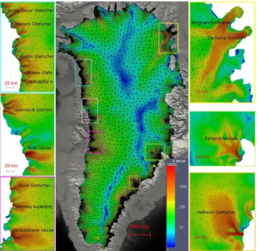
used to adjust the mesh size so that the discretisation error is equi-distributed. First, we mesh the 2-D-footprint of the GrIS. The metric tensor is based on the Hessian matrix of observed surface velocities (Joughin et al., 2010) shown in Fig. 1a. The mesh size is optimised before the simulation using the freely available software YAMS (Frey and Alauzet, 2005). The mesh size decreases from 40 km in the central part of the ice

20

sheet to a minimum resolution of 1 km in the outlet glaciers as shown in Fig. 2. The mesh is then vertically extruded using 16 layers. The resulting 3-D mesh is composed of 417 248 nodes and 748 575 wedge elements.

The bedrock and surface topography are taken from the freely available SeaRise 1 km present-day data set and are based on the Bamber et al. (2001) digital-elevation

25

(8)

TCD

6, 2789–2826, 2012

Title Page

Tables Figures

◭ ◮

Back Close

Full Screen / Esc

Discussion

P

a

per

|

Dis

cussion

P

a

per

|

Discussion

P

a

per

|

Discussio

n

P

a

per

|

3 Initial state

As ice-sheet responses include long timescales (multi-century), forecasting change on decadal-to-century timescales is essentially a short-term forecast and thus simulating the present conditions is crucial. Available observations of the curent state of the ice sheet include the ice-sheet geometry (bedrock and free-surface elevations, e.g.

Bam-5

ber et al., 2001), surface velocities (e.g. Joughin et al., 2010) and rate of change of the surface elevation (e.g. Pritchard et al., 2009). If timeseries of these observations are available for the last decade, observed changes in velocity and surface elevation are certainly the results of transient boundary forcings that are still not fully understood and modelled. Moreover, so far, inverse methods applied to full-Stokes ice-sheet modelling

10

are restricted to diagnostic simulations and are not able to assimilate timeseries. As a consequence, we use here two inverse methods to constrain the basal friction field (βin Eq. 7) from a given geometry and surface velocity field, considered as representa-tive of present day conditions (Sect. 3.1). Due to ice flux divergence anomalies caused by the remaining uncertainties (Seroussi et al., 2011), the free-surface-elevation

rate-15

of-change computed in diagnostic is unphysical, and the available observations are not used here to constrain the model. The free surface elevation is then allowed to diverge from the observations with a relaxation period of 50 yr (Sect. 3.2). The performance of the model to simulate present day conditions is then assessed by comparison of the estimated ice discharge for the main outlets (Rignot and Kanagaratnam, 2006).

20

3.1 Inverse methods

Two variational inverse methods (Arthern and Gudmundsson, 2010; Morlighem et al., 2010) are used to infer the basal friction coefficient field β(x,y) and are compared in the following. Both methods are based on the minimisation of a cost function that measures the mismatch between modelled and observed velocities. The two methods

25

(9)

TCD

6, 2789–2826, 2012

Title Page

Tables Figures

◭ ◮

Back Close

Full Screen / Esc

Discussion

P

a

per

|

Dis

cussion

P

a

per

|

Discussion

P

a

per

|

Discussio

n

P

a

per

|

3.1.1 Robin inverse method

We briefly review the method detailed in Arthern and Gudmundsson (2010). The method consists in solving alternatively theNeumann-type problem, defined by Eq. (4) and the boundary conditions Eqs. (6) and (7), and the associatedDirichlet-type prob-lem, defined by the same equations except that the Neumann upper-surface condition

5

(Eq. 6) is replaced by a Dirichlet condition where observed surface horizontal velocities are imposed.

The cost function that expresses the mismatch between the solutions of the two models is given by

J_o=

Z

Γs

(uN−uD)·(σN−σD)·ndΓ, (9)

10

where superscripts N and D refer to the Neumann and Dirichlet problem solutions, respectively.

The G ˆateaux derivative of the cost functionJ_owith respect to the friction parameter

βfor a perturbationβ′is given by:

dβJo=

Z

Γb

β′(|uD|2− |uN|2)dΓ, (10)

15

where the symbol|.|defines the norm of the velocity vector and_Γ_bis the lower surface. Note that this derivative is exact only for a linear rheology and thus Eq. (10) is only an approximation of the true derivative of the cost function when using Glen’s flow law (Eq. 1) withn >1 in Eq. (2).

3.1.2 Control inverse method

20

(10)

TCD

6, 2789–2826, 2012

Title Page

Tables Figures

◭ ◮

Back Close

Full Screen / Esc

Discussion

P

a

per

|

Dis

cussion

P

a

per

|

Discussion

P

a

per

|

Discussio

n

P

a

per

|

computation of the adjoint of the Stokes system. Here, as in Morlighem et al. (2010), we assume that the sti_ffness matrix of the Stokes system is independent of the velocity and thus self-adjoint, which is exact only for a Newtonian rheology, i.e. whenn=1 in Eq. (2).

As the direction of the ice velocity is mainly governed by the ice-sheet topography,

5

here, we express the cost function as the difference between the norm of the modelled and observed horizontal velocities as

Jo=

Z

Γs

1 2

|u_H| − |uobs_H |2dΓ, (11)

whereuobsare the observed velocities and subscriptH refers to the horizontal compo-nent of the velocity vector.

10

The G ˆateaux derivative is obtained as

d_βJ_o=

Z

Γb

−β′u·λdΓ, (12)

withλthe solution of the adjoint system of the Stokes equations.

Again, this derivative is exact only for a linear rheology and thus is only an approx-imation of the true derivative of the cost function when using Glen’s flow law (Eq. 1)

15

withn >1 in Eq. (2).

3.1.3 Regularisation

To avoid unphysical negative values of the friction parameter,βis expressed as

(11)

TCD

6, 2789–2826, 2012

Title Page

Tables Figures

◭ ◮

Back Close

Full Screen / Esc

Discussion

P

a

per

|

Dis

cussion

P

a

per

|

Discussion

P

a

per

|

Discussio

n

P

a

per

|

The optimisation is now done with respect toα and the G ˆateaux derivative ofJ_o with respect toα is obtained as:

d_αJo=dβJo

dβ

dα. (14)

A Tikhonov regularisation term penalising the spatial first derivatives ofα is added to the cost function:

5

J_reg=1

2 Z

Γb

_∂α

∂x

2

+

_∂α

∂y

2

dΓ. (15)

The G ˆateaux derivative ofJ_regwith respect toα for a perturbationα′is obtained as

d_αJ_reg=

Z

Γb

_∂α

∂x

∂α′ ∂x

+

_∂α

∂y

∂α′ ∂y

dΓ. (16)

The total cost function now writes

J_tot=Jo+λJreg, (17)

10

whereλis a positive ad-hoc parameter. The minimum of this cost function is no longer the best fit to observations, but a compromise (through the tuning ofλ) between fit to observations and smoothness inα.

3.1.4 Minimisation

At the surface of an ice sheet, the magnitude of the velocities di_ffers by several order

15

(12)

TCD

6, 2789–2826, 2012

Title Page

Tables Figures

◭ ◮

Back Close

Full Screen / Esc

Discussion

P

a

per

|

Dis

cussion

P

a

per

|

Discussion

P

a

per

|

Discussio

n

P

a

per

|

size in the original fixed-step gradient descent algorithm (Arthern and Gudmundsson, 2010). Here, when discretising the G ˆateaux derivatives, Eqs. (14) and (16), on the finite element mesh, the continuous scalar product represented by the integral onΓbis trans-formed in a discrete euclidean product. The area surrounding each finite element node on_Γ_b is then included in the gradients used for the minimisation. This leads to good

5

convergence properties with our unstructured mesh as large elements correspond to low velocity areas, and vice versa.

The minimisation of the cost functionJ_tot with respect toα is done using the limited memory quasi-Newton routine M1QN3 (Gilbert and Lemar ´echal, 1989) implemented in Elmer in reverse communication. This method uses an approximation of the second

10

derivatives of the cost function and is then more efficient than a fixed-step gradient descent.

3.1.5 Results

The observed velocities, shown in Fig. 1a, are a compilation of data sets obtained from RADARSAT data at different dates during the first decade of the 2000’s (Joughin et al.,

15

2010). We choose this compilation as it gives the best coverage. For glaciers that have been accelerating, it therefore provides a kind of average value for this period. But for these glaciers, the surface topography has also diverged from the surface topography used here. A proper comparison of the model results with observations of the 2000’s would therefore require coherent data sets for both the topography and the velocities,

20

which are currently not available. For the inversion, gaps in data have been filled by the balance velocities available in the SeaRise dataset.

To compare the performance of the applied inverse methods and also the initialisa-tion of the basal fricinitialisa-tion coefficientβ, the initial friction field is given by

β(x,y)=max(10−4, min(1.0/U_bal, 10−1)) MPa a−1 (18)

25

for the Robin inverse method whereUbalis the balance velocity, and by

(13)

TCD

6, 2789–2826, 2012

Title Page

Tables Figures

◭ ◮

Back Close

Full Screen / Esc

Discussion

P

a

per

|

Dis

cussion

P

a

per

|

Discussion

P

a

per

|

Discussio

n

P

a

per

|

for the control inverse method.

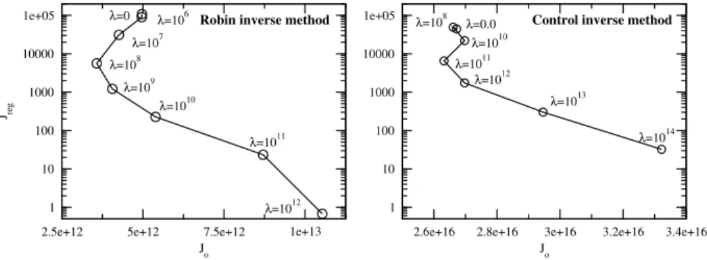
The optimal regularisation parameter λ in Eq. (17) is chosen using the L-curve method. The L-curve is a plot of the optimised variable smoothness, i.e. the termJ_reg

in Eq. (17), as a function of the mismatch between the model and the observations, i.e. the termJo in Eq. (17). The L-curve obtained with both methods is given in Fig. 3.

5

The termJ_reg is identical for the two methods, whereasJ_o is not (Eqs. 9 and 11). This leads to different values of the regularisation parameterλin Eq. (17), which allows to tune the weight of the regularisation with respect toJo. For the Robin inverse method,

when increasingλfrom 0 to 109, the roughness of the basal friction field, represented byJ_reg, decreases by several orders of magnitude with a small decrease of the

mis-10

match between the model and the observation, represented by Jo. This decrease of

J_o may be due to the fact that the gradient used in the model, Eq. (10), is not the true gradient ofJ_odue to the non linearity of the ice rheology. The regularisation, for which the gradient is exact, therefore improves the convergence properties of the model. For higher values ofλ, J_reg still decreases but with a concomitant increase of Jo as the

15

basal friction field becomes too smooth. The L-curves obtained with the two methods are very similar. The minimumJo is obtained for the same order of magnitude ofJreg. The optimal value forλis chosen as the minimum value ofJ_o, i.e. λ_Robin=108 for the Robin inverse method, andλ_CI=1011 for the control inverse method.

The surface velocity field obtained after optimisation of the basal friction field with the

20

Robin inverse method is shown in Fig. 2. Our implementation reproduces very well the observed large-scale flow features (Fig. 1a) with low velocities in the interior and areas of rapid ice flow, restricted to the observed outlet glaciers, near the margins. The largest outlets (Jakobshavn Isbrae, Kangerlugssuaq, Helheim, . . . ) and their catchments are well captured by the anisotropic mesh and the modelled velocity pattern is in good

25

agreement with the observations. Smaller outlet glaciers down to few kilometers in width are also individually distinguishable.

(14)

TCD

6, 2789–2826, 2012

Title Page

Tables Figures

◭ ◮

Back Close

Full Screen / Esc

Discussion

P

a

per

|

Dis

cussion

P

a

per

|

Discussion

P

a

per

|

Discussio

n

P

a

per

|

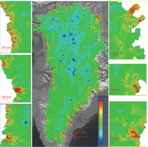
error varies by several order of magnitude between the interior and the margins. The relative error is only few percents in most of the interior where ice is flowing faster than few meters per year. This error is usually higher very locally near the margins. The highest relative errors are located in the North in Peterman Glacier and in the North-East Greenland ice stream where long floating tongues are present but not explicitly

5

taken into account in this application of the model. The remaining di_fferences between modelled and observed velocities can come from three main reasons:

(i) non convergence of the minimisation: it has been shown on twin experiments where the minimum is known (Arthern and Gudmundsson, 2010), that the gradi-ents of the cost function derived analyticaly for a linear rheology, Eqs. (10) and

10

(12), work well in practice with a non-linear rheology. But there is no guaranty in general that the actual minimum will be found (Goldberg and Sergienko, 2011), especially in real applications where the curvature of the cost function is very low.

(ii) Remaining uncertainties: adjusting the sliding coefficient can compensate only partly for errors associated with the uncertainties on the other model parameters

15

and data.

(iii) Unsufficient resolution of the model where the minimum mesh resolution is lower than those of the velocity data, so that the model will not be able to capture all details, especially for the smallest outlets; and of the data as, for example, the ice thickness is not sufficiently known in most outlets.

20

It is difficult to test the first hypothesis as the minimum is unknown but both the cost function and the norm of the gradient decrease during the minimisation and both in-verse methods leads to very similar results (not shown for the Control inin-verse methods), so that we are confident to be close to the actual minimum. Errors shown in Figs. 4 and 5 account both for the error on the direction and on the magnitude of the modelled

25

(15)

TCD

6, 2789–2826, 2012

Title Page

Tables Figures

◭ ◮

Back Close

Full Screen / Esc

Discussion

P

a

per

|

Dis

cussion

P

a

per

|

Discussion

P

a

per

|

Discussio

n

P

a

per

|

flow direction. The cost function used with the Control inverse method only accounts for the di_fference between the velocity norms and not for the direction. Both inverse methods lead to similar errors so that we assume that most of the absolute error is representative of the error on the velocity norm. For the outlets, a common feature, not shown here, is that model velocities are lower than the observations along the central

5

flow lines but higher along the shear margins. This can be explained by unsufficient res-olution of the model and/or of the data, or remaining uncertainties on the ice viscosity for example.

3.2 Relaxation

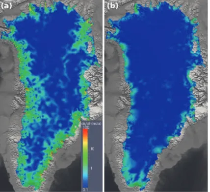
When running prognostic simulations from this initialisation, the free-surface elevation

10

shows unphysical very high rates of change essentially on the margins (Fig. 6). The free surface of the ice sheet is therefore allowed to relax during a 50-yr time-dependent run, forced by a constant present-day climate (Ettema et al., 2009).

One contribution to these initial surface changes comes from ice flux divergence anomalies (Seroussi et al., 2011) due to uncertainties on the bed topography and on

15

the model parameters. These anomalies disappear very quickly within a few years. Another contribution results from the fact that the lateral side of the mesh does not cor-respond exactly to the current position of the fronts of the marine terminated glaciers for which we have no compilation for the whole GrIS. Due to these geometry problems at the front, the ice discharge at the beginning of the relaxation is strongly underestimated

20

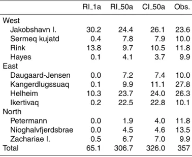
for most of the smallest outlets (Table 2). The mass balance being largely positive due to the SMB term, this results in a thickening of the outlets, until the time when the ice fronts open to evacuate the mass excess.

At the end of the relaxation, the surface velocities, given in Fig. 1b, still show good agreement with the observations, with ice discharge still concentrated in known

out-25

(16)

TCD

6, 2789–2826, 2012

Title Page

Tables Figures

◭ ◮

Back Close

Full Screen / Esc

Discussion

P

a

per

|

Dis

cussion

P

a

per

|

Discussion

P

a

per

|

Discussio

n

P

a

per

|

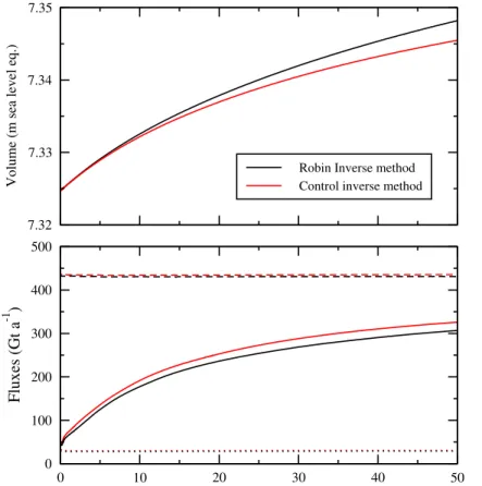
Rignot and Kanagaratnam (2006) for 1996, or 2000 when not available). A detailed comparison shows generally good agreement in areas where the bed topography is well known (e.g., Jakobshavn Isbrae, Helheim Glacier). Agreement is less good in the North where the floating tongues in the model still show a large imbalance of the free surface. The total computed discharge for the relaxed solution is around 300 Gt a−1. Up

5

to now, the magnitude of the computed ice discharge in a continental ice-sheet model has only been addressed by Price et al. (2011) by tuning the boundary condition at the ice front to reproduce the observations only on three major outlets.

The various terms of the mass balance equation during the relaxation are given in Fig. 7. The ice extent does not evolve much during this relaxation and, as a

conse-10

quence, the surface mass balance is constant and equal to 400 Gt a−1. The ice dis-charge increases very quickly during the first twenty years to reach 200 Gt a−1. After, the ice discharge increase slows down. The relaxation is stopped after 50 yr. At this time, the rate of increase of the ice discharge is around 1 Gt a−2. The free surface is nearly at equilibrium except in a few areas near the margins but the rate of change is

15

of the same order of magnitude as the accumulation/ablation (Fig. 6). For the reasons cited previously, Peterman Glacier and the North East Greenland Ice Stream are the most imbalanced at the end of the relaxation. The change in surface elevation between the beginning and the end of the relaxation exceeds several hundred meters in some places. This difference is large but is of the same order of magnitude as the

uncer-20

tainty on the ice thickness in some areas of the GrIS margins. This remains the main limitation of the model where only the upper surface is adjusted whereas most of the uncertainties come from the bed elevation. Future work might consider to use the bed elevation as a control variable as in Pralong and Gudmundsson (2011), and will benefit from new observations. During this relaxation the ice volume increases by less than

25

(17)

TCD

6, 2789–2826, 2012

Title Page

Tables Figures

◭ ◮

Back Close

Full Screen / Esc

Discussion

P

a

per

|

Dis

cussion

P

a

per

|

Discussion

P

a

per

|

Discussio

n

P

a

per

|

The evolution of the total volume and ice discharge obtained with the basal friction field optimised with the two inverse methods are very similar. This is true for each individual outlet as shown in Table 2. The two inverse methods perform similarly and neither can be favoured in view of these results or in terms of computation performance.

4 Sensitivity experiments

5

We use the relaxed solution of the Robin inverse method as the starting point to inves-tigate the GrIS mass balance over one century.

4.1 Set-up

The climate forcing impacts ice dynamics through the net accumulation rate at each surface mesh node. Two SMB scenarios are used, the first (C1), corresponds to

keep-10

ing present conditions (Ettema et al., 2009) constant with time; the second (C2) repre-sents an ensemble of 18 climate models forced under the IPCC A1B emission scenario. Here, we especially focus on the GrIS dynamical response to an increase in basal lu-brication. Perturbations are introduced by applying several homogeneous changes in the basal friction coe_fficientβ; firstly, no perturbation withβ unmodified from the

orig-15

inal inversion (BF1); secondly, a constant perturbation withβdivided by two and then kept constant (BF2); lastly, a continuously enhanced perturbation with β reduced by one order of magnitude over one century (BF3). This last scenario is not unrealistic, as has been shown for a surging glacier (Jay-Allemand et al., 2011),βcan vary by several orders of magnitude with only small changes in the water pressure. Further

destabil-20

(18)

TCD

6, 2789–2826, 2012

Title Page

Tables Figures

◭ ◮

Back Close

Full Screen / Esc

Discussion

P

a

per

|

Dis

cussion

P

a

per

|

Discussion

P

a

per

|

Discussio

n

P

a

per

|

4.2 Results

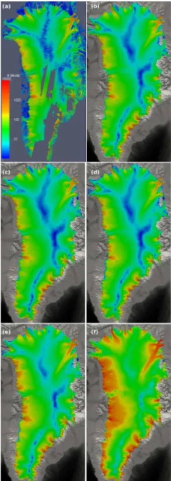
We evaluate the results of the perturbations by considering ice-flow velocities (Fig. 1), the ice-sheet total mass balance (Fig. 8), discharge values from the main outlet glaciers (Table 3) and free-surface-elevation rate-of-change (Fig. 9). For the ice-sheet total mass balance (Fig. 8), we present the total ice-sheet volume and volume change from

5

the starting point, converted to sea-level equivalents (Fig. 8a). The annual mass bal-ance (MB, Fig. 8b) is obtained as the time derivative of the ice-sheet volume. D is computed as the ice flux through the lateral boundary and SMB as the accumula-tion/ablation flux trough the upper surface (Fig. 8c). The difference between MB and SMB-D is the ice flux lost through the bottom boundary (see Sect. 2.1, discussion on

10

boundary condition Eq. 7). In all the applications it corresponds approximately to 10 % of D.

With constant conditions (C1 BF1), the model tends to reach a steady state where the modelled discharge balances the current SMB (430 Gt a−1, Fig. 8c). Neither the ice-sheet extent, nor the surface velocity pattern, change dramatically during this

ex-15

periment (Fig. 1c) and the ice-discharge shows a small increase in the main outlets (Table 3).

The climatic perturbation used here (SMB scenario C2) shows a reduction of SMB of approximately only 100 Gt a−1 after one century (Fig. 8c), which is a lower bound of the forecast given by current climate models (Fettweis et al., 2008). Changes in the

20

marginal extent between the three perturbation experiments detailed below lead to only small differences in the total SMB after one century (Fig. 8c). These differences are one order of magnitude lower than those between the various climate models (Fettweis et al., 2008). Other retro-actions could arise from surface elevation changes but this could be constrained more precisely only by coupling ice-sheet and climate models.

25

(19)

TCD

6, 2789–2826, 2012

Title Page

Tables Figures

◭ ◮

Back Close

Full Screen / Esc

Discussion

P

a

per

|

Dis

cussion

P

a

per

|

Discussion

P

a

per

|

Discussio

n

P

a

per

|

trend over the century (Fig. 8b); in consequence the total ice volume is nearly con-stant (Fig. 8a). For this experiment, the velocity pattern (Fig. 1d) remains similar to the present one. The increase of ablation for this climate scenario is higher in West Greenland. This leads to thinning of the marginal ice in this area, resulting in a re-treat of land-termined glaciers and in a decrease in ice discharge of marine terminated

5

glaciers (Table 3).

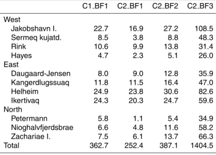
With a constant dynamic perturbation (C2 BF2), halvingβbefore the simulation re-sults in an almost immediate doubling of the ice discharge bringing it close to 500 Gt a−1 (Fig. 8c), in agreement with current estimates based on observations (Rignot et al., 2011). The computed total discharge decreases throughout the 100-yr simulation at

10

a rate equivalent to the rate of decrease of SMB except during the first decade where it decreases faster probably as a reaction to the initial perturbation (Fig. 8c). As a re-sult, after the first decade the annual mass balance shows no particular trend (Fig. 8b) and the ice sheet loses mass at a nearly constant rate (Fig. 8a). For this experiment, we see increased velocities on the interior of each drainage basin (Fig. 1e). This

pat-15

tern is expected if the excess runoff produced by the increase of the ablation area reaches the bed enhancing basal lubrication. As a result of this acceleration, land-terminated glaciers in the west coast do not retreat but again, the reduction of the discharge throughout the simulation is higher in this area.

With an increasing dynamic perturbation (C2 BF3), the discharge increases

contin-20

uously from 300 Gt a−1 to 1400 Gt a−1after 100 yr (Fig. 8c), and the ice sheet is losing mass throughout the 100-yr simulation (Fig. 8a, b). For this experiment, the velocity pat-tern at the end of the century (Fig. 1f), shows large areas of high velocities (>100 m a−1) far inland of each glacier. This scenario seems unlikely if e_fficient drainage systems can develop, reducing the basal sliding (Schoof, 2010). However, it shows that, under

25

(20)

TCD

6, 2789–2826, 2012

Title Page

Tables Figures

◭ ◮

Back Close

Full Screen / Esc

Discussion

P

a

per

|

Dis

cussion

P

a

per

|

Discussion

P

a

per

|

Discussio

n

P

a

per

|

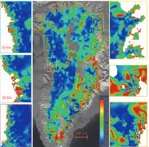
BF3, Fig. 8c), highlight the need to better constrain the spatial and temporal variability of the processes affecting the basal and seaward boundary conditions of the ice sheet. Together with surface velocities, rates of change of the free surface elevation are nowadays widely measured and available (Pritchard et al., 2009). All the glaciers that have been accelerating recently also show a dynamical thinning. Even if these

obser-5

vations have been used by flow models as a post-validation to try to discriminate the destabilising processes (Nick et al., 2009; Price et al., 2011), they have not been used in a proper inverse method so far. Because the homogeneous dynamical perturbation applied here is probably too crude, we do not compare our results to observations but provide a qualitative discussion of the surface elevation changes computed after 10 yr

10

of simulations (Fig. 9).

With experiment C1 BF1, as discussed previously, some drainage basins are still not at equilibrium and their outlets are still thickening due to an SMB higher than the computed discharge. In the interior, the surface elevation change is nearly zero. With a climate perturbation only, i.e. experiment C2 BF1, the margins in the west and south

15

east are thinning and the thickening of Peterman Glacier and the North East Green-land Ice Stream is less pronounced. These differences with experiment C1 BF1 mostly come from the change in the SMB term.

Experiments with a dynamical perturbation, i.e C2 BF2 and C2 BF3, show an addi-tional dynamical thinning associated with the acceleration of the ice, upstream of each

20

drainage basin. Downstream, near the margins, this gives two di_fferent behaviours. (i) If the decrease of the basal friction coefficient also produces an acceleration and an increase of the discharge sufficient to offset the mass excess coming from upstream, the whole ice stream shows a dynamical thinning. This is the case in the south east, and for the Jakobshavn Isbrae and the Heilhem Glacier. (ii) If the acceleration and the

25

(21)

TCD

6, 2789–2826, 2012

Title Page

Tables Figures

◭ ◮

Back Close

Full Screen / Esc

Discussion

P

a

per

|

Dis

cussion

P

a

per

|

Discussion

P

a

per

|

Discussio

n

P

a

per

|

In some aspects, these results therefore agree with observations and show an in-teresting regional variability of the response to the dynamical perturbation. The link between surface runo_ff, basal hydrology and basal sliding will have to be investigated more in-depth to make quantitative comparisons.

5 Conclusions

5

We have shown that our implementation of a model with the correct treatment of lon-gitudinal stresses, sufficient resolution to resolve medium to small outlet glaciers, and a careful initialisation of ice-flow parameters alllows to satisfy the essential pre-requisite of simulating the present-day conditions.

More specific projections will arise as the ice sheet is driven by more complete

10

and precise climate scenarios, and with greater understanding of processes. Our new-generation continental-scale ice-sheet model is well suited to incorporate such informa-tion as it becomes available. However, our current model experiments are significant and general conclusion can already be drawn. The results confirms that the overall mass balance of the GrIS is likely to result, not only from changing SMB, but in large

15

parts, from ice discharge. Our model shows a rapid adjustment of the ice discharge in response to dynamical perturbations. This is supported by other models that in-clude processes at the ice front (Nick et al., 2009) and by recent observations (Howat et al., 2007). We find that SMB changes significantly affect ice discharge on the cen-tury timescale, so that discharge and SMB anomalies can not be treated separetely to

20

estimate the GrIS contribution to sea-level rise. Indeed, results show that, unless the perturbation is continuously enhanced, an increase of the surface ablation reduces the discharge, stabilising the ice sheet. However, in our experiments with constant basal conditions, the rate of decrease of the discharge and of SMB are similar, resulting in a constant annual mass balance. Extrapolating this result to the currently observed

25

(22)

TCD

6, 2789–2826, 2012

Title Page

Tables Figures

◭ ◮

Back Close

Full Screen / Esc

Discussion

P

a

per

|

Dis

cussion

P

a

per

|

Discussion

P

a

per

|

Discussio

n

P

a

per

|

bound given by Price et al. (2011) assuming a self-similar response of the ice sheet to a 10 yr-recurring forcing in the future decades. Conversely, if the perturbation is contin-uously increased, there is su_fficient ice available to sustain the current rate of increase in discharge over an entire century. Taking a discharge anomaly of 100 Gt a−1 increas-ing at rate of 10 Gt a−2for present day, leads by itself to a contribution to sea-level rise

5

of 166 mm in one century. This value is on the lowest half of the values obtained from kinematic considerations assuming low (93 mm) and high (467 mm) scenarios (Pfeffer et al., 2008).

Acknowledgements. This work was supported by both the ice2sea project funded by the Euro-pean Commission’s 7th Framework Programme through grant number 226375 (Ice2sea contri-10

bution number ice2sea052) and the ADAGe project (ANR-09-SYSC-001) funded by the Agence National de la Recherche (ANR). Hakime Seddik and Ralf Greve were supported by a Grant-in-Aid for Scientific Research A (No. 22244058) from the Japan Society for the Promotion of Science (JSPS). We thank I. Joughin for providing the surface velocity data and the SeaRISE community for the compilation of topography and climate forcing data sets. We also thank J. 15

Ruokolainen and P. R ˚aback for their continuous support in developing Elmer. This work was performed using HPC resources from GENCI-CINES (Grant /2011016066/) and from the Ser-vice Commun de Calcul Intensif de l’Observatoire de Grenoble (SCCI).

20

(23)

TCD

6, 2789–2826, 2012

Title Page

Tables Figures

◭ ◮

Back Close

Full Screen / Esc

Discussion

P

a

per

|

Dis

cussion

P

a

per

|

Discussion

P

a

per

|

Discussio

n

P

a

per

|

References

Alley, R. B. and Joughin, I.: Modeling ice-sheet flow, Science, 336, 551–552,

doi:10.1126/science.1220530, 2012. 2792

Arthern, R. J. and Gudmundsson, G. H.: Initialization of ice-sheet forecasts viewed as an in-verse Robin problem, J. Glaciol., 56, 527–533, 2010. 2792, 2796, 2797, 2800, 2802

5

Bamber, J. L., Layberry, R. L., and Gogineni, S. P.: A new ice thickness and bed data set for the Greenland ice sheet 1. Measurement, data reduction, and errors, J. Geophys. Res., 106, 33773–33780, 2001. 2795, 2796

Ettema, J., van den Broeke, M. R., van Meijgaard, E., van de Berg, W. J., Bamber, J. L., Box, J. E., and Bales, R. C.: Higher surface mass balance of the Greenland ice 10

sheet revealed by high-resolution climate modeling, Geophys. Res. Lett., 36, L12501, doi:10.1029/2009GL038110, 2009. 2803, 2805

Favier, L., Gagliardini, O., Durand, G., and Zwinger, T.: A three-dimensional full Stokes model of the grounding line dynamics: effect of a pinning point beneath the ice shelf, The Cryosphere, 6, 101–112, doi:10.5194/tc-6-101-2012, 2012. 2794

15

Fettweis, X., Hanna, E., Gall ´ee, H., Huybrechts, P., and Erpicum, M.: Estimation of the Green-land ice sheet surface mass balance for the 20th and 21st centuries, The Cryosphere, 2, 117–129, doi:10.5194/tc-2-117-2008, 2008. 2806

Frey, P. and Alauzet, F.: Anisotropic mesh adaptation for CFD computations, Comput. Method Appl. M., 194, 5068–5082, doi:10.1016/j.cma.2004.11.025, 2005. 2792, 2795

20

Gilbert, J. C. and Lemar ´echal, C.: Some numerical experiments with variable-storage quasi-Newton algorithms, Math. Program., 45, 407–435, doi:10.1007/BF01589113, 1989. 2800 Glen, J. W.: The creep of polycrystalline ice, P. Roy. Soc. Lond. A Mat., 228, 519–538,

doi:10.1098/rspa.1955.0066, 1955. 2793

Goldberg, D. N. and Sergienko, O. V.: Data assimilation using a hybrid ice flow model, The 25

Cryosphere, 5, 315–327, doi:10.5194/tc-5-315-2011, 2011. 2802

Greve, R.: Application of a polythermal three-dimensional ice sheet model to the Greenland ice sheet: response to steady-state and transient climate scenarios, J. Climate, 10, 901–918, 1997. 2794

Greve, R. and Blatter, H.: Dynamics of Ice Sheets and Glaciers, Springer, Berlin, Germany etc., 30

(24)

TCD

6, 2789–2826, 2012

Title Page

Tables Figures

◭ ◮

Back Close

Full Screen / Esc

Discussion

P

a

per

|

Dis

cussion

P

a

per

|

Discussion

P

a

per

|

Discussio

n

P

a

per

|

Howat, I. M., Joughin, I., and Scambos, T. A.: Rapid changes in ice discharge from Greenland outlet glaciers, science, 315, 1559–1561, doi:10.1126/science.1138478, 2007. 2791, 2792, 2809

Jay-Allemand, M., Gillet-Chaulet, F., Gagliardini, O., and Nodet, M.: Investigating changes in basal conditions of Variegated Glacier prior to and during its 1982–1983 surge, The 5

Cryosphere, 5, 659–672, doi:10.5194/tc-5-659-2011, 2011. 2792, 2805

Joughin, I., Smith, B. E., Howat, I. M., Scambos, T., and Moon, T.: Greenland flow variability from ice-sheet-wide velocity mapping, J. Glaciol., 56, 415–430, 2010. 2791, 2795, 2796, 2800

Little, C. M., Oppenheimer, M., Alley, R. B., Balaji, V., Clarke, G. K. C., Delworth, T. L., 10

Hallberg, R., Holland, D. M., Hulbe, C. L., Jacobs, S., Johnson, J. V., Levy, H., Lip-scomb, W. H., Marshall, S. J., Parizek, B. R., Payne, A. J., Schmidt, G. A., Stouffer, R. J., Vaughan, D. G., and Winton, M.: Toward a new generation of ice sheet models, Eos, 88, 578, doi:10.1029/2007EO520002, 2007. 2792

MacAyeal, D. R.: A tutorial on the use of control methods in ice-sheet modeling, J. Glaciol., 39, 15

91–98, 1993. 2797

Moon, T., Joughin, I., Smith, B., and Howat, I.: 21st-century evolution of Greenland outlet glacier velocities, Science, 336, 576–578, doi:10.1126/science.1219985, 2012. 2791, 2792

Morlighem, M., Rignot, E., Seroussi, H., Larour, E., Dhia, H. B., and Aubry, D.: Spatial patterns of basal drag inferred using control methods from a full-Stokes and simpler models for Pine 20

Island Glacier, West Antarctica, Geophys. Res. Lett., 37, 6, doi:10.1029/2007EO520002, 2010. 2792, 2796, 2797, 2798

Nick, F. M., Vieli, A., Howat, I. M., and Joughin, I.: Large-scale changes in Green-land outlet glacier dynamics triggered at the terminus, Nat. Geosci., 2, 110–114, doi:10.1038/NGEO394, 2009. 2791, 2808, 2809

25

Pattyn, F., Perichon, L., Aschwanden, A., Breuer, B., de Smedt, B., Gagliardini, O., Gudmunds-son, G. H., Hindmarsh, R. C. A., Hubbard, A., JohnGudmunds-son, J. V., Kleiner, T., Konovalov, Y., Mar-tin, C., Payne, A. J., Pollard, D., Price, S., R ¨uckamp, M., Saito, F., Souˇcek, O., Sugiyama, S., and Zwinger, T.: Benchmark experiments for higher-order and full-Stokes ice sheet models (ISMIP–HOM), The Cryosphere, 2, 95–108, doi:10.5194/tc-2-95-2008, 2008. 2792

30

(25)

TCD

6, 2789–2826, 2012

Title Page

Tables Figures

◭ ◮

Back Close

Full Screen / Esc

Discussion

P

a

per

|

Dis

cussion

P

a

per

|

Discussion

P

a

per

|

Discussio

n

P

a

per

|

Pralong, M. R. and Gudmundsson, G. H.: Bayesian estimation of basal conditions on Rutford Ice Stream, West Antarctica, from surface data, J. Glaciol., 57, 315–324, 2011. 2804 Price, S. F., Payne, A. J., Howat, I. M., and Smith, B. E.: Committed sea-level rise for the next

century from Greenland ice sheet dynamics during the past decade, P. Natl. Acad. Sci. USA, 108, 8978–8983, doi:10.1073/pnas.1017313108, 2011. 2792, 2804, 2808, 2810

5

Pritchard, H. D., Arthern, R. J., Vaughan, D. G., and Edwards, L. A.: Extensive dynamic thin-ning on the margins of the Greenland and Antarctic ice sheets, Nature, 461, 971–975, doi:10.1038/NGEO394, 2009. 2791, 2796, 2808

Rignot, E. and Kanagaratnam, P.: Changes in the velocity structure of the Greenland Ice Sheet, Science, 311, 986–990, doi:10.1126/science.1121381, 2006. 2796, 2804, 2816

10

Rignot, E., Velicogna, I., van den Broeke, M. R., Monaghan, A., and Lenaerts, J.: Acceleration of the contribution of the Greenland and Antarctic ice sheets to sea level rise, Geophys. Res. Lett., 38, L05503, doi:10.1029/2011GL046583, 2011. 2790, 2807, 2809

Sch ¨afer, M., Zwinger, T., Christoffersen, P., Gillet-Chaulet, F., Laakso, K., Pettersson, R., Po-hjola, V. A., Strozzi, T., and Moore, J. C.: Sensitivity of basal conditions in an inverse 15

model: Vestfonna Ice-Cap, Nordaustlandet/Svalbard, The Cryosphere Discuss., 6, 427–467, doi:10.5194/tcd-6-427-2012, 2012. 2799

Schoof, C.: Ice-sheet acceleration driven by melt supply variability, Nature, 468, 803–806, doi:10.1038/nature09618, 2010. 2791, 2807

Schrama, E. J. O. and Wouters, B.: Revisiting Greenland ice sheet mass loss observed by 20

GRACE, J. Geophys. Res., 116, B02407, doi:10.1029/2009JB006847, 2011. 2790

Seddik, H., Greve, R., Zwinger, T., Gillet-Chaulet, F., and Gagliardini, O.: Simulations of the Greenland ice sheet 100 years into the future with the full Stokes model Elmer/Ice, J. Glaciol., 58, 427–440, doi:10.3189/2012JoG11J177, 2012. 2792, 2794

Seroussi, H., Morlighem, M., Rignot, E., Larour, E., Aubry, D., Dhia, H. B., and Kristensen, S. S.: 25

Ice flux divergence anomalies on 79 north Glacier, Greenland, Geophys. Res. Lett., 38, 5, doi:10.1029/2009JB006847, 2011. 2792, 2796, 2803

Solomon, S., Qin, D., Manning, M., Chen, Z., Marquis, M., Averyt, K. B., Tignor, M., and Miller, H. L.: Contribution of Working Group I to the Fourth Assessment Report of the In-tergovernmental Panel on Climate Change, 2007, Cambridge University Press, Cambridge, 30

2007. 2792

(26)

TCD

6, 2789–2826, 2012

Title Page

Tables Figures

◭ ◮

Back Close

Full Screen / Esc

Discussion

P

a

per

|

Dis

cussion

P

a

per

|

Discussion

P

a

per

|

Discussio

n

P

a

per

|

van den Broeke, M., Bamber, J., Ettema, J., Rignot, E., Schrama, E., van de Berg, W. J., van Meijgaard, E., Velicogna, I., and Wouters, B.: Partitioning recent Greenland mass loss, Science, 326, 984–986, doi:10.1126/science.1178176, 2009. 2790

Van Der Veen, C. J., Plummer, J. C., and Stearns, L. A.: Controls on the recent speed-up of Jakobshavn Isbrae, West Greenland, J. Glaciol., 57, 770, 2011. 2791

5

Vaughan, D. G. and Arthern, R.: Why is it hard to predict the future of ice sheets?, Science, 315, 1503–1504, doi:10.1126/science.1141111, 2007. 2791

Wouters, B., Chambers, D., and Schrama, E. J. O.: GRACE observes small-scale mass loss in Greenland, Geophys. Res. Lett, 35, L20501, doi:10.1029/2008GL034816, 2008. 2790

Zwally, H. J., Abdalati, W., Herring, T., Larson, K., Saba, J., and Steffen, K.:

Sur-10

(27)

TCD

6, 2789–2826, 2012

Title Page

Tables Figures

◭ ◮

Back Close

Full Screen / Esc

Discussion

P

a

per

|

Dis

cussion

P

a

per

|

Discussion

P

a

per

|

Discussio

n

P

a

per

|

Table 1.List of parameter values used in this study.

Parameters Values Units

E 2.5

A_o(T <−10◦C) 3.985×10−13 Pa−3s−1 A_o(T >−10◦C) 1.916×103 Pa−3s−1

Q(T <−10◦C) −60 kJ mol−1

Q(T >−10◦C) −139 kJ mol−1

g 9.8 m s−2

n 3

ρ_w 1025 kg m−3

ρi 910 kg m−

(28)

TCD

6, 2789–2826, 2012

Title Page

Tables Figures

◭ ◮

Back Close

Full Screen / Esc

Discussion

P

a

per

|

Dis

cussion

P

a

per

|

Discussion

P

a

per

|

Discussio

n

P

a

per

|

Table 2. Model discharge for individual outlets and the whole ice sheet in Gt a−1: after 1 yr (RI 1a) and after 50 yr (RI 50a) of surface relaxation with the Robin inverse method, after 50 yr of surface relaxation with the control inverse method (CI 50a), and observations from 1996 (or 2000 when not available) (Rignot and Kanagaratnam, 2006) (Obs.).

RI 1a RI 50a CI 50a Obs.

West

Jakobshavn I. 30.2 24.4 26.1 23.6

Sermeq kujatd 0.4 7.8 7.9 10.0

Rink 13.8 9.7 10.5 11.8

Hayes 0.1 4.1 3.7 9.9

East

Daugaard-Jensen 0.0 7.2 7.4 10.0

Kangerdlugssuaq 0.1 9.9 11.1 27.8

Helheim 10.3 23.7 24.0 26.3

Ikertivaq 0.2 22.5 22.8 10.1

North

Petermann 0.0 1.9 4.0 11.8

Nioghalvfjerdsbrae 0.0 4.5 4.6 13.5

Zachariae I. 0.5 6.7 7.0 9.9

(29)

TCD

6, 2789–2826, 2012

Title Page

Tables Figures

◭ ◮

Back Close

Full Screen / Esc

Discussion

P

a

per

|

Dis

cussion

P

a

per

|

Discussion

P

a

per

|

Discussio

n

P

a

per

|

Table 3.Model discharge for individual outlets and the whole ice sheet in Gt a−1 after one century for the various experiments.

C1 BF1 C2 BF1 C2 BF2 C2 BF3

West

Jakobshavn I. 22.7 16.9 27.2 108.5

Sermeq kujatd. 8.5 3.8 8.8 48.3

Rink 10.6 9.9 13.8 31.4

Hayes 4.7 2.3 5.1 26.0

East

Daugaard-Jensen 8.0 9.0 12.8 35.9

Kangerdlugssuaq 11.8 11.5 16.4 47.0

Helheim 24.9 23.8 30.6 82.6

Ikertivaq 24.3 20.3 24.7 59.6

North

Petermann 5.8 1.1 5.4 34.9

Nioghalvfjerdsbrae 6.6 4.8 11.6 58.2

Zachariae I. 7.5 6.1 13.7 66.3

(30)

TCD

6, 2789–2826, 2012

Title Page

Tables Figures

◭ ◮

Back Close

Full Screen / Esc

Discussion

P

a

per

|

Dis

cussion

P

a

per

|

Discussion

P

a

per

|

Discussio

n

P

a

per

|

Fig. 1.GrIS surface velocities.(a)Observed surface velocities on the original regular 500 m×

500 m grid; Computed surface velocities:(b)after relaxation; after one century for(c)

(31)

TCD

6, 2789–2826, 2012

Title Page

Tables Figures

◭ ◮

Back Close

Full Screen / Esc

Discussion

P

a

per

|

Dis

cussion

P

a

per

|

Discussion

P

a

per

|

Discussio

n

P

a

per

|

(32)

TCD

6, 2789–2826, 2012

Title Page

Tables Figures

◭ ◮

Back Close

Full Screen / Esc

Discussion

P

a

per

|

Dis

cussion

P

a

per

|

Discussion

P

a

per

|

Discussio

n

P

a

per

|

2.6e+16 2.8e+16 3e+16 3.2e+16 3.4e+16 J

o 1

10 100 1000 10000 1e+05

2.5e+12 5e+12 7.5e+12 1e+13 J

o 1

10 100 1000 10000 1e+05

Jreg

λ=0.0

λ=108

λ=1010

λ=1011

λ=1012

λ=1013

λ=1014

λ=1010

λ=1012

λ=109

λ=108

λ=107

λ=106

λ=0

λ=1011

Robin inverse method Control inverse method

(33)

TCD

6, 2789–2826, 2012

Title Page

Tables Figures

◭ ◮

Back Close

Full Screen / Esc

Discussion

P

a

per

|

Dis

cussion

P

a

per

|

Discussion

P

a

per

|

Discussio

n

P

a

per

|

(34)

TCD

6, 2789–2826, 2012

Title Page

Tables Figures

◭ ◮

Back Close

Full Screen / Esc

Discussion

P

a

per

|

Dis

cussion

P

a

per

|

Discussion

P

a

per

|

Discussio

n

P

a

per

|