An ice sheet model of reduced complexity for paleoclimate studies

(1)

ESDD

6, 1395–1443, 2015

An ice sheet model of reduced complexity

for paleoclimate studies

B. Neffet al.

Title Page

Abstract Introduction

Conclusions References

Tables Figures

◭ ◮

Back Close

Full Screen / Esc

Printer-friendly Version

Interactive Discussion

Discussion

P

a

per

|

Discussion

P

a

per

|

Discussion

P

a

per

|

Discussion

P

a

per

Earth Syst. Dynam. Discuss., 6, 1395–1443, 2015 www.earth-syst-dynam-discuss.net/6/1395/2015/ doi:10.5194/esdd-6-1395-2015

This discussion paper is/has been under review for the journal Earth System Dynamics (ESD). Please refer to the corresponding final paper in ESD if available.

An ice sheet model of reduced complexity

for paleoclimate studies

B. Neff1,2, A. Born1,2, and T. F. Stocker1,2

1

Climate and Environmental Physics, Physics Institute, University of Bern, Bern, Switzerland

2

Oeschger Centre for Climate Change Research, Bern, Switzerland

Received: 9 July 2015 – Accepted: 19 July 2015 – Published: 11 August 2015

Correspondence to: A. Born (born@climate.unibe.ch)

(2)

ESDD

6, 1395–1443, 2015

B. Neffet al.

Title Page

Tables Figures

◭ ◮

Back Close

Full Screen / Esc

Discussion

P

a

per

|

Discussion

P

a

per

|

Discussion

P

a

per

|

Discussion

P

a

per

|

Abstract

IceBern2D is a vertically integrated ice sheet model to investigate the ice distribution on

long timescales under different climatic conditions. It is forced by simulated fields of

sur-face temperature and precipitation of the last glacial maximum and present day climate from a comprehensive climate model. This constant forcing is adjusted to changes in

5

ice elevation. Bedrock sinking and sea level are a function of ice volume. Due to its

reduced complexity and computational efficiency, the model is well-suited for

exten-sive sensitivity studies and ensemble simulations on extenexten-sive temporal and spatial scales. It shows good quantitative agreement with standardized benchmarks on an ar-tificial domain (EISMINT). Present day and last glacial maximum ice distributions on

10

the Northern Hemisphere are also simulated with good agreement. Glacial ice volume in Eurasia is underestimated due to the lack of ice shelves in our model.

The efficiency of the model is utilized by running an ensemble of 400 simulations

with perturbed model parameters and two di_fferent estimates of the climate at the last

glacial maximum. The sensitivity to the imposed climate boundary conditions and the

15

positive degree day factorβ, i.e., the surface mass balance, outweighs the influence of

parameters that disturb the flow of ice. This justifies the use of simplified dynamics as

a means to achieve computational efficiency for simulations that cover several glacial

cycles. The sensitivity of the model to changes in surface temperature is illustrated as a hysteresis based on 5 million year long simulations.

20

1 Introduction

The understanding of the Earth’s climate on time scales longer than about 100 000 years (100 kyr) critically depends on the build-up and demise of continental ice sheets. Over the past several million years, its number alternated between the two that are present today on Greenland and Antarctica and four, with two additional masses of

25

(3)

ESDD

6, 1395–1443, 2015

B. Neffet al.

Title Page

Tables Figures

◭ ◮

Back Close

Full Screen / Esc

Discussion

P

a

per

|

Discussion

P

a

per

|

Discussion

P

a

per

|

Discussion

P

a

per

level to drop in excess of 120 m during the most recent glaciation (Waelbroeck et al., 2002), exposing currently submerged land that allowed humans to first arrive and settle on the American (Dixon, 2001) and Australian continents (Forster, 2004).

Proxy records from deep sea sediments show that ice volume varied predominantly on time scales of 41 kyr between 3 and 0.8 million years ago, and with a 100 kyr

period-5

icity more recently (Lisiecki and Raymo, 2005). This is somewhat inconsistent with the prevailing theory that ice sheet volume is dominated by the intensity of Northern Hemi-sphere summer insolation causing ice to melt (Milankovitch, 1941), because summer insolation on the Northern Hemisphere varies predominantly on the precessional time scale of 23 kyr (Berger, 1978).

10

Several ice sheet-climate interactions have been proposed to explain this nonlinear response of ice volume to the orbital forcing. Besides the closure of ocean pathways mentioned above, the rerouting of freshwater by ice sheets also has a profound impact on the ocean circulation and sea ice distribution (Stocker, 2013), potentially chang-ing moisture availability for ice sheet growth (Gildor and Tziperman, 2001). Similarly,

15

meridional water transport from the tropics to high latitudes, arguably controlled by in-solation gradients instead of absolute values, has been suggested as a limiting factor of ice sheet growth (Raymo and Nisancioglu, 2003). Topographic changes due to the accumulation of ice changes the atmospheric circulation on local (Merz et al., 2014a, b) and hemispheric scales (Li and Battisti, 2008; Pausata et al., 2011; Merz et al., 2013).

20

As ice sheets are usually brighter than the surface they replace, they impact the plane-tary radiation balance in the short wavelength part of the spectrum (Cess et al., 1991). The long wavelength radiation balance also changes with the growth of ice sheets as the concentration of atmospheric greenhouse gases closely follows global ice sheet volume (Loulergue et al., 2008; Lüthi et al., 2008; Schilt et al., 2010). Probable causes

25

(4)

ESDD

6, 1395–1443, 2015

B. Neffet al.

Title Page

Tables Figures

◭ ◮

Back Close

Full Screen / Esc

Discussion

P

a

per

|

Discussion

P

a

per

|

Discussion

P

a

per

|

Discussion

P

a

per

|

Although these basic components are easily understood at their individual level, the full picture is very complex so that comprehensive numerical modeling is necessary to quantify the underlying physical processes. The often prohibitive cost to run cli-mate models over periods of several millennia has limited such attempts to either using somewhat arbitrary methods to reduce simulation time (e.g., Herrington and Poulsen,

5

2011; Abe-Ouchi et al., 2013; Heinemann et al., 2014) or the use of climate models of reduced complexity (e.g., Gallée et al., 1992; Smith et al., 2003; Charbit et al., 2007; Bonelli et al., 2009; Robinson et al., 2011). However, in spite of their focus on

nu-merical e_fficiency, the ice sheet models used in some of the latter studies rival their

climate model counterparts in complexity and computational cost, which is not justified

10

for all applications. Importantly, the use of complex ice sheet and ice shelf dynamics consumes resources that in specific cases would better be used for advanced surface mass balance schemes or a probabilistic analysis of many repeated simulations.

In this study, we present a vertically integrated ice sheet model (IceBern2D) that is

e_fficient enough to add only a small computational overhead even to the fastest coarse

15

resolution climate models. This enables simulations spanning several glacial cycles. Similar models that have successfully been employed in the past on a hemispheric scale (Neeman et al., 1988; Verbitsky and Oglesby, 1992) and for regional applications (Oerlemans, 1981a; Siegert and Marsiat, 2001; Plummer and Phillips, 2003; Näslund et al., 2003). The dynamics are similar to early one-dimensional models (Oerlemans,

20

1981b, 1982), but calculated on a two-dimensional grid. This type of model has been found to produce results similar to three-dimensional thermomechanical models (Calov and Marsiat, 1998).

The IceBern2D model is described in detail in Sect. 2. It is found to perform well in idealized experiments (EISMINT, Huybrechts et al., 1996, Sect. 3) as well as in

simula-25

tions under continuous Last Glacial Maximum (LGM) and preindustrial climate forcing

(Sect. 4.2). We take advantage of the efficiency of the model by using a large

(5)

ESDD

6, 1395–1443, 2015

B. Neffet al.

Title Page

Tables Figures

◭ ◮

Back Close

Full Screen / Esc

Discussion

P

a

per

|

Discussion

P

a

per

|

Discussion

P

a

per

|

Discussion

P

a

per

experiments of five million years duration (Sect. 4.3). We summarize and discuss these results in Sect. 5 and provide an outlook on future directions in Sect. 6.

2 Model formulation

The IceBern2D model is designed to investigate the two dimensional flow of ice and

its distribution under di_fferent climatic conditions. Therefore, the physical basis of the

5

model is focused on the most important processes. It is based on the conservation of mass and simulates the ice flow in two dimensions, the vertical flow of ice is not simulated explicitly. The forcing of the model is deliberately chosen to only include precipitation and temperature in order to allow for a wide range of usage scenarios with coupled and uncoupled climate models, observational data and possibly climate

10

proxy reconstructions.

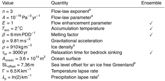
The model is based on different physical and empirical constants. Empirical

con-stants are primarily determined from present-day conditions and may vary under dif-ferent climates and geographical locations. Therefore, these values are used as tuning

parameters for different simulations in a common ensemble and marked in Table 1.

15

The IceBern2D model is discretized on a C-grid (Arakawa and Lamb, 1977). The staggered C-grid is characterized by a combination of calculated values at the cen-ter and the border of the grid. This combination yields the most stable results in our simulations.

2.1 Ice dynamics

20

The basis of the model is formed by the conservation of ice volume in time (Oerlemans,

1981b; Huybrechts et al., 1996). The rate of change of ice thickness h with time is

formulated as

∂h

(6)

ESDD

6, 1395–1443, 2015

B. Neffet al.

Title Page

Tables Figures

◭ ◮

Back Close

Full Screen / Esc

Discussion

P

a

per

|

Discussion

P

a

per

|

Discussion

P

a

per

|

Discussion

P

a

per

|

where SMB represents the annual net surface mass balance which is described in

Sect. 2.2. The flow of ice takes the form of a di_ffusion with the nonlinear di_ffusivity D

detailed below and the gradient of the ice surface elevationZ a.s.l.. Z is the sum of

bedrock elevationB and ice thicknessh. The vector differential operator (∇) is defined

for the two lateral dimensions.

5

The diffusivity D is calculated from Glen’s flow law (Glen, 1955) by assuming that

longitudinal stresses can safely be neglected over the much higher shearing of hori-zontal planes. This is the so-called “shallow ice approximation” (Hutter, 1983) that can be justified by the fact that the grid spacing is at least a factor of ten greater than the vertical extension of the ice. To obtain the ice volume flow, the flow law is integrated

10

over the full height (Huybrechts et al., 1996) so that:

D=2E A(ρg)

n

n+2 h

n+2

"

∂Z ∂x

2 +

∂Z ∂y

2#

(n−1)

2

, (2)

whereAand nare two empirical parameters determined from a power-law fit of strain

rate and effective shear stress. A generally depends on the temperature of the ice

which can not be calculated here due to the missing vertical coordinate. We therefore

15

chose a constant value. The plasticity and hence its flow velocity can be modified by

an empirical enhancement parameterE which is commonly used to parameterize the

softer, impurity-rich glacial ice (Fisher and Koerner, 1986).ρ andg are the density of

ice and the gravitational acceleration, respectively (Table 1).

Bedrock relaxation 20

Thick ice sheets exert a substantial mass load on the underlying bedrock. This leads in equilibrium to an isostatic sinking of the bedrock by about one third, corresponding to

the inverse ratio of rock and ice density ρrock

ρ_ice ≈3, the hydrostatic equilibrium. This is an

important mechanism because it influences the melting of the ice. When the bedrock yields under the pressure of the ice, the top of the ice sheet sinks to a lower and warmer

(7)

ESDD

6, 1395–1443, 2015

B. Neffet al.

Title Page

Tables Figures

◭ ◮

Back Close

Full Screen / Esc

Discussion

P

a

per

|

Discussion

P

a

per

|

Discussion

P

a

per

|

Discussion

P

a

per

position. The temperature difference promotes melting and thereby feeds back to the

surface mass balance.

A simple yet effective formulation of the bedrock adjustment is the exponential

sink-ing toward its hydrostatic equilibrium (Oerlemans, 1981b):

∂B ∂t =−τ

−1 br

_ρ

rock

ρ_ice h+B−B0

. (3)

5

Bis the bedrock elevation, B₀is the elevation of the bedrock without ice load andh

represents the ice thickness. The relaxation timeτbr represents a characteristic time

it takes to restore equilibrium. A common value forτ_br for is 3000 years (Huybrechts,

2002), but the value may vary locally. Thereforeτ_bris used as a tuning parameter here

(Table 3). Equation (3) is a simplified representation of mass flow in the Earth’s upper

10

mantle. It only a_ffects the local grid point and no surrounding fields which is considered

sufficient for the purpose of an ice sheet model of reduced complexity.

For the elevation of the bedrock without ice load (B0) ETOPO1 (Amante and Eakins,

2009) is used. ETOPO1 has a resolution of one arc-minute and distinguishes between bedrock and ice surface. For our application the resolution is linearly interpolated to

15

a stereographic grid of 40 km resolution. It is assumed that ice and bedrock in

Green-land are close to isostatic equilibrium today. Thus,B₀is estimated by adding one third

of the ice thickness to the bedrock elevation which corresponds to the mentioned in-verse ratio of rock and ice density. In the model domain and at 40 km resolution, this

adjustment of the bedrock only a_ffects Greenland.

20

2.2 Surface mass balance

The surface mass balance (SMB), the difference of the accumulation and ablation,

determines where the ice sheet gains or loses mass and thereby drives the flow of the ice sheet. SMB is calculated from daily surface air temperature and precipitation fields. These data are obtained from simulations using the Community Climate System Model

25

(8)

ESDD

6, 1395–1443, 2015

B. Neffet al.

Title Page

Tables Figures

◭ ◮

Back Close

Full Screen / Esc

Discussion

P

a

per

|

Discussion

P

a

per

|

Discussion

P

a

per

|

Discussion

P

a

per

|

Accumulation is the cumulative precipitation below 0◦C. However, the use of daily

averages does not account for potentially lower temperatures during the night that may be below freezing. Also, precipitation at temperatures above the melting point might refreeze upon contact with the cold snow surface. Thus, the sensitivity of the

accumu-lation temperatureT_accis tested and used to tune the model.

5

Melting of the ice is parameterized with the positive degree day method (Reeh,

1991). For each grid point, daily average temperatures above 0◦C are integrated over

one year to obtain the positive degree days (PDD) as a simplified measure of the en-ergy available for melting. This number is then multiplied with the melting parameter

βto calculate the mass loss.β is an empirical constant that accounts for the e_ffect of

10

the local climate and the surface radiation balance. Thus, it is known to largely vary with changing surface conditions, including the density of the surface snow or ice, the

presence of meltwater and other effects on the local albedo (Braithwaite, 1995; Charbit

et al., 2013). To partially account for these e_ffects, many studies employ two individual

melting parameters for snow and bare ice (Huybrechts and T’siobbel, 1995; Huybrechts

15

and de Wolde, 1999). The extent and volume of simulated ice sheets is very sensitive to the choice of melting parameters (Ritz et al., 1997). For the present study, we ne-glect these complications in spite of their possibly important impact on the sensitivity of the simulated ice sheets. Therefore, only one melting parameter is used for ice. As

with the accumulation temperature, the sensitivity of the ice sheet toβ is also tested

20

and used for tuning purposes (Table 3).

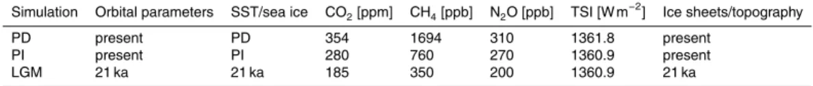
Climate forcing for preindustrial (PI) and glacial (LGM) climates is provided by sim-ulations with the atmosphere component of CCSM4 (Gent et al., 2011; Neale et al., 2013) (Table 2), which have been analyzed and validated earlier by Hofer et al. (2012) and Merz et al. (2013). The lower boundary conditions for the sea surface are derived

25

(9)

ESDD

6, 1395–1443, 2015

B. Neffet al.

Title Page

Tables Figures

◭ ◮

Back Close

Full Screen / Esc

Discussion

P

a

per

|

Discussion

P

a

per

|

Discussion

P

a

per

|

Discussion

P

a

per

of the simulations are extracted to force the ice sheet model. The spatial resolution is 0.9◦×1.25◦.

All simulated climate variables are referenced to the continental surface in the rela-tively coarse grid of the climate model. This does not not concur with the more finely resolved topography of the ice sheet model, in particular since the growth of ice entails

5

considerable changes in the surface elevation. Thus, after a bilinear interpolation from the climate model to the ice sheet model grid, the climatological fields of surface air

temperature are corrected for altitude with a constant lapse rate_{Γ =}−6.5×10−3K m−1:

T_ISM(t)=T_GCM+ Γ·(Z_ISM(t)−Z_GCM), (4)

whereZ_GCMis the elevation of the interpolated climate model grid,Z_ISM(t) is the

time-10

dependent elevation of the ice sheet model surface, and analogously for T_GCM and

T_ISM(t). This correction is applied throughout the ice sheet model simulation to account

for changes in ice surface topography.

Precipitation is corrected with a height-desertification effect: values above Z₀=

2000 m are halved every 1000 m (Budd and Smith, 1979). The precipitation rateP_ISM

15

at the height of the ice sheetZ_ISM is derived from the precipitation of the GCM

precipi-tationP_GCMas follows:

PISM=PGCM·exp(−λp(max(ZISM,Z0)−max(ZGCM,Z0))) (5)

with λ_p=ln(2)/1000 m. Z₀ refers to the initial surface elevation in the first time step

without ice,Z_GCMis the surface elevation used in the GCM simulation from the climate

20

input. All used constants are in Table 1.

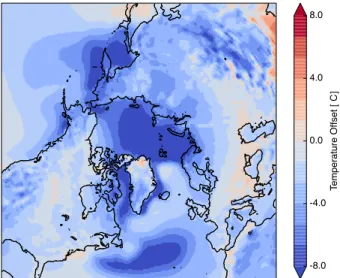
Comparison of the present day simulation of CCSM4 with reanalyzed data from ERA-Interim (Dee et al., 2011) reveals considerable temperature biases. The CCSM3 sim-ulation which is used as ocean forcing for the CCSM4 simsim-ulations overestimates the amount of sea ice in the Northern Hemisphere (Collins et al., 2006), causing too cold

25

temperatures in these areas (Fig. 1). The anomalies range from−12.5 to+5.5◦C with

(10)

ESDD

6, 1395–1443, 2015

B. Neffet al.

Title Page

Tables Figures

◭ ◮

Back Close

Full Screen / Esc

Discussion

P

a

per

|

Discussion

P

a

per

|

Discussion

P

a

per

|

Discussion

P

a

per

|

To remove this shortcoming of the lower boundary conditions from the simulations, the bias is subtracted from the daily temperature fields after interpolation to the ice sheet grid but before the lapse rate correction. The influence of this correction is

in-vestigated by forcing the ice sheet model with both the corrected (LGM_bs, bs=bias

subtracted) and uncorrected (LGM_uc, uc₌uncorrected) surface climate fields. The

pre-5

cipitation is not altered in any simulation concerning this temperature bias. But note that

the ratio of solid to liquid precipitation of the accumulation is affected by the

tempera-ture change.

2.3 Model domain

The domain of the model is limited to the Northern Hemisphere because approximately

10

80 % of the changes in ice volume during the LGM took place on the Northern Hemi-sphere (Clark and Mix, 2002). A polar azimuthal projection is used as grid base. The lateral grid is identical to the one of SICOPOLIS (Greve, 1997; Born et al., 2010).

The spatial resolution is 40 km×40 km. Each grid cell has exactly one vertical layer

which stores all information such as ice thickness, accumulation, ablation. An ice mask

15

is introduced to reduce cost-intensive ice flux calculations to grid cells with ice instead of the entire model domain. The temporal resolution is one year which makes it impos-sible to implement a seasonal cycle in the SMB.

The SMB of the Himalayas is not well represented in the current model version. The simplified ablation scheme does not explicitly account for melting by shortwave

radia-20

tion at subzero temperatures and large intra-day and intra-seasonal variations in both

accumulation and melting. Both e_ffects are more important at the subtropical latitude

of the Himalayas than further north where glacier growth and decay are confined to two individual seasons. Thus, in the Himalayas, the approach used here leads to an unrealistically high accumulation rate, which destabilizes the model. For this reason,

25

(11)

ESDD

6, 1395–1443, 2015

B. Neffet al.

Title Page

Tables Figures

◭ ◮

Back Close

Full Screen / Esc

Discussion

P

a

per

|

Discussion

P

a

per

|

Discussion

P

a

per

|

Discussion

P

a

per

Sea level

The changing sea level during the simulations has a large influence on the ice flow, since some shallow bays fall dry and provide the possibility for the ice to cover new

areas, for example the Baltic Sea or the Great Banks o_ffNewfoundland.

All simulations start without any ice in the Northern Hemisphere which leads to an

5

offset in sea level compared to today’s situation. This offset of 7.36 m (Table 1) is equiv-alent to the ice volume on Greenland, the major storage in the Northern Hemisphere, would melt (Bamber et al., 2013). The change of the global mean sea level is re-trieved by dividing the water equivalent of the total ice volume by the ocean area of

3.625×1014m2 (IPCC, 2007). All ice volumes in this work are presented as sea level

10

equivalent (SLE). The initial positive o_ffset from Greenland of 7.36 m is added to all sea

levels, therefore, an ice-free Northern Hemisphere is not equal to 0 m SLE.

Ice shelves are not simulated. Ice is assumed to calve into the ocean upon contact with the shoreline, approximated by setting the ice thickness to zero at these points.

This may yield to less ice in the coastal areas for neglecting the buttressing effect of

15

ice shelves (Dupont and Alley, 2005). However, to avoid overly rapid ice loss due to rising sea level, already existing ice is allowed to persist unless it starts to float. If the

existing ice column with a density of 910 kg m−3 is able to displace the water column

between the bedrock and sea level, i.e., the hydrostatic equilibrium is not yet reached, the ice is still treated as grounded and the grid point is equivalent to land. As soon as

20

the mass of the water column exceeds the ice mass, all ice is removed and the grid cell is converted to a water cell.

3 Test cases on a square domain

In order to test the present model formulation, we perform a series of benchmark ex-periments defined by the European Ice Sheet Modelling INiTiative (EISMINT)

(12)

ESDD

6, 1395–1443, 2015

B. Neffet al.

Title Page

Tables Figures

◭ ◮

Back Close

Full Screen / Esc

Discussion

P

a

per

|

Discussion

P

a

per

|

Discussion

P

a

per

|

Discussion

P

a

per

|

brechts et al., 1996). To validate our model and their results, both the fixed-margin

(EISMINT_fixed) and moving-margin (EISMINT_freemargin) experiments are carried out.

EISMINT_fixed uses a flat bed without relaxation. It prescribes a constant SMB of

0.3 m yr−1 in the entire domain. The shape of the simulated ice sheet is

symmet-ric, ruling out inconsistencies in the grid configuration (Fig. 2, left). Our experiment

5

EISMINT_fixed is indistinguishable from the reference (Huybrechts et al., 1996). Both

peaks in the center of the area are 3342.6 m above ground.

The second benchmark EISMINT_freemargin also uses a flat rigid bed. Here, the SMB

linearly decreases from the center of the grid toward the boundaries. This pattern is point-symmetric around the central point so that the SMB function resembles an upright

10

cone. Thus, the IceBern2D simulation is also symmetric with respect to the center of the model domain (Fig. 2, right). Again, we find very close agreement with the results of Huybrechts et al. (1996), with a deviation of less than 1 % in the elevation of the central peak. This confirms the validity of the formulation and implementation of the IceBern2D model. In the next section we apply our model to climatically relevant configurations and

15

conditions.

4 Northern Hemisphere ice volume in preindustrial and glacial climates

4.1 Last glacial maximum climate forcing, model tuning

The sensitivity of the IceBern2D model to four empirical model parameters is investi-gated by varying their values within their range of uncertainty (Table 3). There are two

20

parameters that change the surface mass balance (SMB): the melting parameter β

and the accumulation temperatureT_acc. The other two influence the ice flow. The flow

enhancement parameterE linearly modifies the flow-law parameterA(Eq. 2).τ_br

de-termines the relaxation time of the bedrock which influences the ice flow. If the bedrock

stays longer at its initial elevation, the elevation gradient ∇Z is higher (Eq. 2). The

25

(13)

ESDD

6, 1395–1443, 2015

B. Neffet al.

Title Page

Tables Figures

◭ ◮

Back Close

Full Screen / Esc

Discussion

P

a

per

|

Discussion

P

a

per

|

Discussion

P

a

per

|

Discussion

P

a

per

therefore the temperature decreases at the surface when the elevation yields under the ice. A shorter relaxation time leads to a decrease of the SMB. All possible parame-ter perturbations amount to a total of 200 combinations. Each simulation is forced with the two versions of LGM forcing outlined above.

This large number of simulations is evaluated primarily by their simulated total ice

5

volume which is compared to available reconstructions (Denton, 1981; Peltier, 2002; Clark and Mix, 2002; Peltier, 2004). Although the ice sheets in the LGM were not in equilibrium (Clark et al., 2009; Heinemann et al., 2014), the simulations here are forced

with an LGM climate until equilibrium is reached. Therefore, the ice volume may differ

in the simulations compared to LGM reconstructions.

10

The spread of the ice volume in sea level equivalent (SLE) depends significantly on

the climate forcing. For the climate forcing without temperature bias correction (LGM_uc),

the spread of the ice volume is between −270 and −65 m SLE, while the spread for

the bias corrected climate forcing (LGM_bs) is much smaller between−130 and−65 m

(Fig. 4, lower part).

15

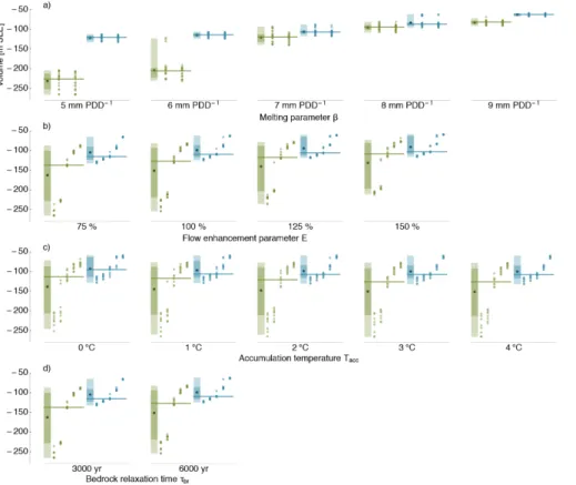
Each tuning parameter (Table 3) has different influences on the maximum volume.

Figure 3 illustrates the tendency and distribution of these tuning parameters. The

melt-ing parameterβhas the strongest influence on ice volume in comparison with other

pa-rameters. The mean sea level, as well as the the 95 percentile, decrease with increases

inβ. This variation between di_fferent values of β is also seen in the other diagrams,

20

where di_fferent values of βare shown as columns of dots. Generally, the width of the

distribution also decreases with increasingβ. A large jump in SLE is observed between

6 and 7 mm PDD−1which is also visible in the density distribution (Fig. 4, lower part).

Simulations with an ice volume above 200 m SLE tend to have aβlower or equal than

7 mm PDD−1with three exceptions.

25

Compared to the impact of β and the climate boundary conditions, the influence

of all other model parameters on ice volume is relatively weak. A weak influence of

the flow enhancement parameterE to maximum ice volume is apparent as faster ice

(14)

ESDD

6, 1395–1443, 2015

B. Neffet al.

Title Page

Tables Figures

◭ ◮

Back Close

Full Screen / Esc

Discussion

P

a

per

|

Discussion

P

a

per

|

Discussion

P

a

per

|

Discussion

P

a

per

|

the upper limit is almost fixed. Therefore, the group of isolated ensemble members

with a lowβ at the upper limit gets closer to the mean values. The mean and median

are closer at a higher ice flux. The influence of the accumulation temperature T_acc

on minimum sea level is very small. Higher Tacc results in a slightly lower sea level,

because it leads to more accumulation. No apparent di_fference is visible between the

5

two bedrock relaxation time scalesτ_br. This result is not unexpected becauseτ_bronly

impacts the transient bedrock sinking during the ice sheet build-up, not the maximum ice volume shown here. The median, mean and also the percentile boxes are similar for both bedrock relaxation times.

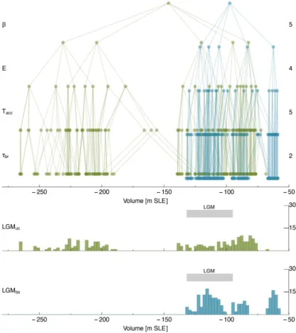
Figure 4 is separated into two parts. Both share the horizontal axis that represents

10

the total ice volume in SLE. The upper part is a tree plot, where each layer repre-sents one specific tuning parameter to illustrate the spread they cause. At the bottom all individual simulations are shown. From bottom to top, simulations are averaged parameter-wise at each level. Thus, the ice volume range caused by variations in each individual tuning parameter is visualized by the divergent lines from the top down. The

15

highest point is the average of all ensemble simulations. The two ensembles are shown

in di_fferent colors as before. As an example, each of the twenty points of one climate

forcing at the third layer from the top represent the average of all combinations ofT_acc

andτ_br. As this level illustrates the impact of E, four points representing the different

considered values of this variable connect into one single dot at their average position

20

of the level above. This yields five di_fferent dots, each representing one of the possible

values ofβ. For better readability, the parameters have been ordered so that the one

with the greatest influence on minimum ice volume is on top (β) and the least sensitive

at the bottom (τ_br). With the information about the tendency of the sea level change

with respect to the parameter variations (Fig. 3) it is possible to address the individual

25

(15)

ESDD

6, 1395–1443, 2015

B. Neffet al.

Title Page

Tables Figures

◭ ◮

Back Close

Full Screen / Esc

Discussion

P

a

per

|

Discussion

P

a

per

|

Discussion

P

a

per

|

Discussion

P

a

per

The tree plot shows that the influence of the tuning parameter has a clear order. Nevertheless, there are a few obvious examples, where the points change the position and join a cluster of another branch. The most prominent example are six simulations

with different bedrock relaxations which have a gap of more than 80 m SLE and each

of them is positioned exactly on one side of the big split. A Longer relaxation time leads

5

to larger ice volumes, because ice sheets can grow faster with a long relaxation time and may stabilize at this larger volume because the surface elevation remains longer at high altitudes with positive SMB.

The density distribution shows a non-normal distribution for every ensemble of

dif-ferent climate forcing. LGM_uchas two obvious groups with a gap of roughly 50 m SLE.

10

The group with the lower sea level consists ofβconfigurations with 5 and 6 mm PDD−1

(see Fig. 3), the group with the upper sea level includes allβgreater and equal than

7 mm PDD−1. Responsible for this gap is the Laurentide ice sheet. During the build-up

process of the Laurentide ice sheet the eastern and western ice streams join together

to a single ice body. Simulations in the LGM_uc ensemble with an ice volume greater

15

than 225 SLE consist of a single Laurentide ice sheet, while simulations with a lower

ice volume these two streams are not in contact with each other. The LGM_bs is also

separated into two groups but the width of the gap is only around 10 m SLE. Again,

the two groups are mostly defined by different values of β and the connection of the

eastern and western ice stream to the Laurentide ice sheet.

20

Figure 4 highlights potential LGM ice volumes (Clark and Mix, 2002) as gray

horizon-tal bars in the density distribution. The lower limit at−95 m SLE is mainly from Peltier

(2002) while the upper limit at−132 m SLE corresponds to the maximum CLIMAP

re-construction (Denton, 1981) for the Northern Hemisphere in each case. The ICE-5G

reconstruction from Peltier (2004) with−117 m SLE is located in the center of the bar.

25

Simulations below this bar are considered as suitable LGM simulations for further

in-vestigations. The LGM_ucensemble has 50 possible LGM simulations while from LGM_bs

(16)

ESDD

6, 1395–1443, 2015

B. Neffet al.

Title Page

Tables Figures

◭ ◮

Back Close

Full Screen / Esc

Discussion

P

a

per

|

Discussion

P

a

per

|

Discussion

P

a

per

|

Discussion

P

a

per

|

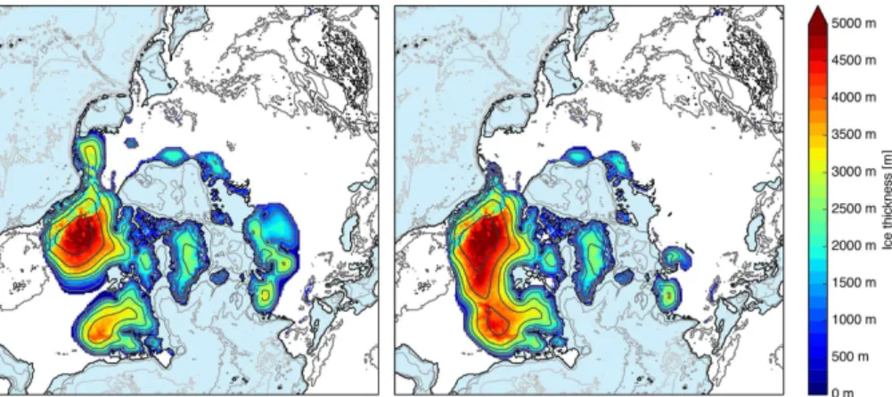
each respective climate forcing look quite different (Fig. 5) although these two

ensem-ble composites di_ffer in their ice volume by only 3 m SLE.

The most obvious difference between the two composites is the Laurentide ice sheet.

The ice flows from two different streams towards the Great Plains. With the LGM_uc

forc-ing, these two streams are not connected in any simulation. A gap in the Great Plains

5

remains. This is due to higher temperatures in the Great Plains in the LGM_uc

ensem-ble than in the corrected version (Fig. 1). Therefore, with LGM_bs forcing, eastern and

western Laurentide ice streams connect easier and faster compared to the uncorrected ensemble but the two domes remain separated. This is consistent with the ICE-5G re-construction that also suggests two distinct domes on the Laurentide ice sheet (Fig. 6,

10

right). However, the separation is probably exaggerated in our simulations because the Hudson Bay remains below sea level and therefore ice-free.

The Eurasian ice sheet accumulates in the LGM_bs less ice compared to the

uncor-rected version. The British Isles and Scandinavia are covered by ice in both ensembles.

The Eurasian ice sheet in the LGM_ucensemble without the temperature bias correction

15

consists of one large ice sheet with a connected and distinct eastern part. Whereas the

ensemble LGM_bs has two individual small Eurasian ice sheets of almost equal

expan-sion. The model accumulates ice in the Alps in both ensembles which are discrete from

other ice masses. The LGM_ucaccumulates more ice in Eurasia and is therefore closer

to ICE-5G. Nevertheless, both climate forcing underestimate the ice volume in Eurasia.

20

The Bering Strait and the Asian far east region in LGM_bs ensemble are similar to

the ICE-5G reconstruction (Fig. 6, right). The LGM_uc ensemble accumulates ice in

the American part of the Bering Strait, whereas the ice in the LGM_bs ensemble and

ICE-5G reconstruction is in this part not that distinct. Ziemen et al. (2014) attributes the overestimated accumulation in this region to the missing albedo variation in their model

25

(17)

ESDD

6, 1395–1443, 2015

B. Neffet al.

Title Page

Tables Figures

◭ ◮

Back Close

Full Screen / Esc

Discussion

P

a

per

|

Discussion

P

a

per

|

Discussion

P

a

per

|

Discussion

P

a

per

Overall, the results with LGM_bsforcing are closer to the LGM reconstruction. Besides

the relatively small Eurasian ice sheet, the ice distribution is closer to ICE-5G in all

considered LGM_bs ensemble members than the ones from the LGM_ucensemble. The

spread of the minimum sea level (Fig. 3) is narrow and more than half of all LGM_bs

simulations are considered valid in terms of minimum LGM sea level compared to only

5

one quarter of all LGM_uc simulations. Therefore, only ensemble LGM_uc is not further

considered in the results section.

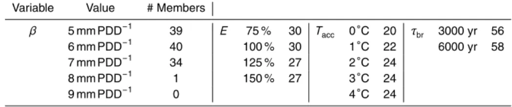
Table 4 shows the distribution of all tuning parameters from all 114 LGM_bs

simula-tions with an ice volume between 95 and 132 m SLE (see Fig. 4). These simulasimula-tions

constitute the ensemble composite from Fig. 5 (right). The distribution ofβhas a clear

10

peak at 6 mm PDD−1 very close to the average of 5.97 mm PDD−1. For the flow

en-hancement factorE, most simulations consistent with reconstructions have values of

75 and 100 % with an average of 111 %. The accumulation temperatureA_temp shows

a slight tendency to warmer temperatures and the two bedrock relaxationsτ_brare

dis-tributed almost equally.

15

Representing the average over a large number of potentially very different

sim-ulations of ice distribution with di_fferent model parameters, the composites are not

physically consistent. Thus, the composite for LGM_bs is now compared with the

equi-librium state of the simulation whose parameters are closest to the mean value of

the parameters of the ensemble composite (β=6 mm PDD−1,E =100 %,T_acc=2◦C,

20

τ_br=3000 yr; Table 4). The situation in Eurasia, Greenland and Bering Strait is very

similar between this simulation (Fig. 6, left) and the ensemble composite (Fig. 5, right).

Nevertheless, there are small di_fferences at the Laurentide ice sheet between these

two results. The single simulation consistent with the approximate mean values shows indications of a single dome Laurentide ice sheet, whereas the two individual domes

25

(18)

ESDD

6, 1395–1443, 2015

B. Neffet al.

Title Page

Tables Figures

◭ ◮

Back Close

Full Screen / Esc

Discussion

P

a

per

|

Discussion

P

a

per

|

Discussion

P

a

per

|

Discussion

P

a

per

|

ICE-5G from Peltier (2004). Therefore, this parameter set is considered as the best-guess tuning parameters (Table 1). For further investigations, only this parameter set is considered.

Simulations at the upper limit of the LGM sea level at 130 m SLE have a similar ice distribution in Eurasia as the simulation with the best guess tuning parameters (not

5

shown). The additional ice volume is mainly due to thicker ice in the same regions as in Fig. 6 (left) and does not add to the ice sheet area. All simulations with realistic LGM sea level underestimate the Eurasian ice sheet.

4.2 Preindustrial climate forcing

The IceBern2D is strongly dependent on the surface mass balance (SMB) and the

10

tuning parametersβandTaccdirectly related to it. To benchmark the best-guess tuning

parameters (values in Table 1) from the LGM_bssimulation, IceBern2D is applied on the

Northern Hemisphere under preindustrial conditions (Table 2).

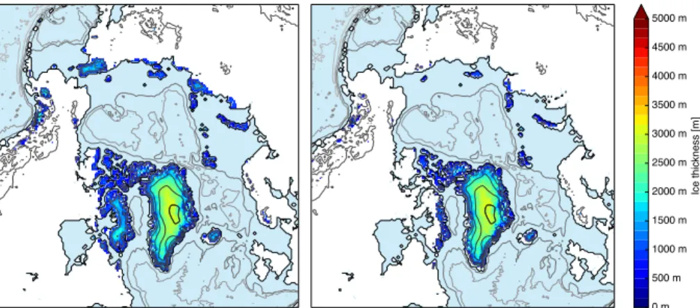
Both versions of preindustrial forcing without the temperature bias (PI_uc and PI_bs)

do not accumulate significant ice volumes in the Northern Hemisphere (Fig. 7) with

15

the best-guess tuning parameters (β=6 mm PDD−1, T_acc=2◦C, E=100 % and τ=

3000 yr). The ice volumes correspond to −8.2 m SLE and −4.1 m SLE, respectively,

with the most suitable tuning parameters where the positive o_ffset of 7.36 m SLE from

Greenland is already subtracted from the values. The most conspicuous difference

be-tween the two climate forcings is on Baffin Islands and Chukotka in far eastern Siberia.

20

The forcing without the temperature bias (PI_bs) accumulates much less ice in this area,

and the result is more realistic. Both climate forcings result in very similar ice volume

of Greenland with 10.0 m SLE (PI_uc) and 9.9 m SLE (PI_bs). This exceeds the ice volume

(19)

ESDD

6, 1395–1443, 2015

B. Neffet al.

Title Page

Tables Figures

◭ ◮

Back Close

Full Screen / Esc

Discussion

P

a

per

|

Discussion

P

a

per

|

Discussion

P

a

per

|

Discussion

P

a

per

4.3 Multiple equilibria in Northern Hemisphere ice volume

One of the primary advantages of the ice sheet model is its computational e_fficiency

and hence the possibility for large ensemble simulations and long integration times. Here, a reduced ensemble of 18 parameter combinations (Table 5) has been forced

with the LGM_bs data and a slowly varying global temperature o_ffset. Temperature

5

anomalies have been linearly decreased from+5 to −5◦C over 2.5 million years and

increased again to +5◦C in the same way. The maximum temperature offset

corre-sponds to the temperature di_fference between the CCSM4 LGM and PI simulation of

4.97 K in the Northern Hemisphere (Table 2). One simulation had numerical instabilities after 4.5 mio years and was not considered in the results.

10

To ensure that the rate of temperature change is slow enough for the ice sheet to re-main in continuous quasi-equilibrium, seven simulations were carried out with the

best-guess parameter set in which the temperature change was interrupted at different

val-ues. These simulations continued with a constant temperature o_ffset for 100 000 years

(Fig. 8, black dots on the right). These interrupted runs confirm that the transient

sim-15

ulation is a good approximation to a continuous equilibrium.

The ice volume as a function of the temperature o_ffset describes a hysteresis (Fig. 8).

There are two stable equilibria for almost every temperature, depending on the initial value of the ice volume. This is valid globally as well as for the individual regions North America and Eurasia (Fig. 8c and d). In contrast to the global ice volumes (a,b), the

20

regional ice volumes in Fig. 8c and d have no global sea level offset of 7.36 m.

Different tuning parameters have a modest influence on the overall shape of the

hys-teresis and major transitions (Fig. 8a). A slight horizontal shift to a later or earlier ice

volume change is visible. Simulations with the same melting parameter β are close

together and identify as three individual groups at the build up of the ice sheet. All 6

25

simulations with a β of 5 mm PDD−1 reach ice volumes greater than 500 m SLE and

(20)

ESDD

6, 1395–1443, 2015

B. Neffet al.

Title Page

Tables Figures

◭ ◮

Back Close

Full Screen / Esc

Discussion

P

a

per

|

Discussion

P

a

per

|

Discussion

P

a

per

|

Discussion

P

a

per

|

illustrates that the open southern boundaries on both major land masses complicate the definition of the hysteresis loop, because the upper limit is not limited by continen-tal boundaries. Nevertheless, the evolution of all ensemble members is similar, which justifies to limit the detailed discussion to the single hysteresis simulations with the best-guess parameter set (Fig. 8b–d)

5

There are three processes which influence rapid ice volume changes. They can be seen in the hysteresis (Fig. 8) as an almost vertical volume change. The most impor-tant influence is the positive ice elevation feedback. As soon as the surface tempera-ture reaches a certain level where the SMB turns positive, the ice sheet grows fast to higher and colder elevations and stabilizes itself. Adjacent areas may be influenced by

10

the ice flow from these newly glaciated regions, so that the SMB turns positive there too. A positive feedback is induced which is much faster compared to the temperature

change of the hysteresis (Fig. 8c, at 2◦C).

Another strong influence during the build up process on the ice volume is the contact of two individual ice sheets over eastern and western North America that combine to

15

form the Laurentide ice sheet. Although we use an idealized forcing, this evolution is consistent with reconstructions of the last glaciation (Stokes et al., 2012; Kleman et al., 2013). The ice volume increases considerably as soon as these two streams connect

with each other (Fig. 8c, at 0.5◦C) because ice flows from two di_fferent directions into

the center of the continent. The connection of these two streams is responsible for the

20

jump of roughly 40 m SLE. The ice volume in North America decreases steadily and relatively slowly on the descending branch of the hysteresis until a positive temperature

offset of 3◦C. At higher temperatures the SMB turns positive in the southern part of

the central Laurentide ice sheet and it retreats quickly, especially the western part disappears almost completely. The eastern part is not in equilibrium with the underlying

25

bedrock after this rapid ice loss. Therefore a small rebound of the ice volume is visible after the ice volume decrease of almost 100 m SLE (Fig. 8c).

(21)

ESDD

6, 1395–1443, 2015

B. Neffet al.

Title Page

Tables Figures

◭ ◮

Back Close

Full Screen / Esc

Discussion

P

a

per

|

Discussion

P

a

per

|

Discussion

P

a

per

|

Discussion

P

a

per

ie. British Isles or Scandinavia, are not able to bypass these barriers because the Ice-Bern2D does not include floating ice shelves. However, if the water level drops below a certain level, areas previously separated by water join and ice can expand into new

regions. The sea level change may have an immediate effect if the ice sheet is already

in contact with the water barrier and can expand in regions that fall dry, e.g., the Great

5

Banks of Newfoundland.

At the beginning of the hysteresis, at temperatures above 2.5◦C, the Northern

Hemi-sphere apart from Greenland is nearly ice free. After one complete hysteresis loop,

most of the simulations reach a similar ice volume at the initial temperature offset of

∆ +5◦C than at the ice free beginning. However, the simulation with the best-guess

10

parameter set does not become ice-free at the end of the hysteresis. Especially the Laurentide ice sheet has still some remarkable volume while the Eurasian ice sheet

disappears around 4◦C (Fig. 8c and d).

The di_fference in ice volume between the ascending and descending branches of

the hysteresis at a temperature o_ffset of _∆T =0◦C, i.e., with the LGM_bs forcing, is

15

123 m SLE. The shape and distribution of the simulated ice sheets on the lower branch of the hysteresis after 1.25 mio years is virtually indistinguishable from the equilib-rium of the simulations with constant forcing shown in Sect. 4.1 (Fig. 6, left). Figure 9

shows the ice thickness for∆T =0◦C after 3.75 mio years on the upper branch of the

hysteresis. All ice masses but Greenland are considerably larger, amounting to about

20

50 m SLE on North America alone. The extent of the Laurentide ice sheet is mostly the same as on the lower branch of the hysteresis as it does not extend further south. The

only major di_fference in ice are is the fully ice-covered Hudson Bay due to the

inter-mittently lower sea level. The ice volume di_fference in Eurasia is roughly 40 m SLE, but

during the build up process Eurasia is nearly ice free. Therefore, the relative difference

25

volume of the hysteresis in Eurasian ice is very large (Fig. 8d). At the LGM temperature

∆T =0◦C on the lower branch, only two small ice sheets are present on Scandinavia

(22)

unrealis-ESDD

6, 1395–1443, 2015

B. Neffet al.

Title Page

Tables Figures

◭ ◮

Back Close

Full Screen / Esc

Discussion

P

a

per

|

Discussion

P

a

per

|

Discussion

P

a

per

|

Discussion

P

a

per

|

tic for the last glaciation and could explain the underrepresented Eurasian ice sheet from the LGM simulations above. Therefore, small temperature or precipitation varia-tions could lead to higher ice masses in Eurasia similar in result to the idealized forcing that causes the hysteresis. This latter simulation resembles the ICE-5G reconstruc-tion more closely (Figs. 9 and 6, right). The addireconstruc-tional 30 m SLE of ice to explain the

5

lower to upper hysteresis difference at∆T=0◦C are found in Siberia which but outside

the region that was covered by the Eurasian ice sheet in reconstructions (see Fig. 9)

(Svendsen et al., 2004). At the same temperature o_ffset, this area is nearly ice free on

the lower branch of the hysteresis.

5 Summary and discussion

10

In this study, we present a model for continental-scale ice sheets that simplifies the dynamics of ice flow into a single, vertically integrated layer. The resulting two-dimensional flow is simulated on a rectangular domain that covers most of the land mass of the Northern Hemisphere. The surface mass balance uses the positive de-gree day method (Reeh, 1991), based on daily fields of surface air temperature and

15

total precipitation from the comprehensive global climate model CESM1 (Gent et al., 2011; Merz et al., 2013). Eustatic sea level and the land mask are prognostically ad-justed as a function of the simulated ice volume.

The simplified dynamics of the ice flow compare favorably in the standardized tests of the EISMINT project (Huybrechts et al., 1996).

20

Similar models have been used to study the last glacial inception in Europe (Oerle-mans, 1981a; Siegert et al., 1999) and the sensitivity of climate-ice sheet interactions during the last glacial cycle (Neeman et al., 1988). Strong adaptations in the present day climate (Siegert and Marsiat, 2001) were necessary to get similar results as LGM reconstructions from Svendsen et al. (2004). However, existing ice sheet models of

re-25

(23)

ESDD

6, 1395–1443, 2015

B. Neffet al.

Title Page

Tables Figures

◭ ◮

Back Close

Full Screen / Esc

Discussion

P

a

per

|

Discussion

P

a

per

|

Discussion

P

a

per

|

Discussion

P

a

per

simulations on a fine grid over the Northern Hemisphere with a precise bedrock and its relaxation have until now not been carried out with a 2D shallow ice approximation model.

Taking advantage of the computational efficiency of the model, a large set of

sim-ulations with perturbed parameters is used to optimize the simulation of Northern

5

Hemisphere ice volume during the Last Glacial Maximum (Peltier, 2004). Results show a reasonable agreement on North America, while the Eurasian ice sheet is too small. This is likely due to the lack of ice shelves in our model that does not allow the Barents Sea to be covered by ice and delays the development of an ice sheet on the Baltic and North Seas until the sea level is low enough for grounded ice to locally grow or advance

10

into the area. This could be a problem as the marine ice sheets of the Barents and Kara Seas have been shown to play a pivotal role early during the last glaciation (Svendsen et al., 2004). On regional scales the missing ice shelf may influence the results, ie. the Hudson Bay would be covered by shelf ice wile it remains ice free in IceBern2D LGM simulations. Furthermore, ice shelves buttress the ice sheet flow (Dupont and Alley,

15

2005). While the fundamentally different stress balance of ice shelves cannot be

in-cluded in our model at this point, one possible solution is to allow the grounded ice to grow into deep water down to a certain water depth (Siegert et al., 1999; Tarasov and Peltier, 1999; Abe-Ouchi et al., 2013). Aside from these shortcomings, the optimized model version yields a realistic modern ice distribution when forced with simulated

20

preindustrial climate from the same model.

The overestimated sea ice in the CCSM simulations (Collins et al., 2006) and the associated temperature bias influences the global ice sheet volume and its

distribu-tion. Simulations forced with the colder uncorrected climate (LGM_uc) have a lower

and a wider distribution of the ice volume. The temperature of the corrected ensemble

25

(LGM_bs) is on average 3◦C warmer. The simulated density distribution of ice volumes

is therefore limited to a smaller bandwidth of a 3◦C warmer climate with an ice free

(24)

ESDD

6, 1395–1443, 2015

B. Neffet al.

Title Page

Tables Figures

◭ ◮

Back Close

Full Screen / Esc

Discussion

P

a

per

|

Discussion

P

a

per

|

Discussion

P

a

per

|

Discussion

P

a

per

|

ensemble overall lead to results which are comparable to LGM reconstructions as ICE-5G.

Although the LGM ice sheet was not in equilibrium (Clark et al., 2009; Heinemann et al., 2014), all simulations are forced until an equilibrium is achieved. It takes around 120 kyr years with a constant climate forcing until a steady state of all ice sheets is

5

reached. LGM cycles in the past 500 kyr years are around 100 kyr years (Hays et al., 1976; Imbrie and Imbrie, 1980), nevertheless, cycles between 80 and 120 kyr are not unusual (Huybers and Wunsch, 2005). During LGM the Laurentide ice sheet was known to be dry (Bromwich et al., 2004), therefore, a constant LGM climate forcing beginning at an ice free hemisphere takes longer to establish a full grown Laurentide

10

ice sheet.

Owing to the focus on simplicity and numerical efficiency, the thermal coupling of

the ice dynamics as well as basal melting are neglected. However, Calov and Mar-siat (1998) showed that vertically integrated models yield results of comparable quality as thermomechanical models. They also conclude that the representation of SMB is

15

more important to simulate the last glacial cycle than the accurate description of ice dynamics. Nevertheless, Johnson and Fastook (2002) state, that basal melting can

have a dramatic e_ffect on the glaciation cycle. It is theoretically possible to approximate

melting at the bottom of the ice sheet by a function based on accumulation rate, tem-perature and geothermal heat flux. However, this could be the subject of further model

20

development.

In long simulations we find multiple equilibria in ice volume, as evidenced by the

hys-teresis. A global temperature o_ffset is applied to the LGM_bs forcing. Starting at₊5◦C,

approximately the di_fference between the simulated LGM and preindustrial climates in

CESM in the ice sheet model domain, the offset linearly decreases to −5◦C over the

25

course of 2.5 million years. The very slow transient temperature change ensures that the simulated ice sheet remains in continuous quasi-equilibrium. Subsequently,

(25)

ESDD

6, 1395–1443, 2015

B. Neffet al.

Title Page

Tables Figures

◭ ◮

Back Close

Full Screen / Esc

Discussion

P

a

per

|

Discussion

P

a

per

|

Discussion

P

a

per

|

Discussion

P

a

per

sheets are found to have at least two stable states over almost the entire temperature o_ffset range.

Ice volume increases and decreases abruptly at several points on the temperature scale. As soon as temperatures are low enough for the local mass balance to become positive, the ice sheet quickly grows to higher, colder elevations and thereby stabilizes

5

itself. This mechanism is consistent with similar simulations of the Cenozoic Antarctic Ice Sheet (Pollard and DeConto, 2005). Importantly, the individual jumps in ice vol-ume depend on the local mass balance and the ice sheet geometry alone, which both are closely related to the bed topography. Variations in the model parameters play a secondary role as they may shift these glaciation and deglaciation events on the

10

temperature scale but do not a_ffect their existence or individual height.

Our hysteresis experiments are similar to simulations by Abe-Ouchi et al. (2013), al-though they employed more comprehensive representations for both climate variations and ice sheet dynamics, and consequentially cannot continuously vary temperature

o_ffsets. We confirm that the hysteresis of the North American ice sheet is located at

15

warmer temperature offsets than the hysteresis of the Eurasian ice sheet. Also, the

retreating North American ice sheet is most sensitive to temperature increase when its volume is between 120 and 50 m SLE. Disagreement is found for the Eurasian ice sheet, as our model does not find a rapid retreat for rising temperatures. The simulated volume is generally lower here. This is likely due to the inadequate representation of

20

marine ice sheets in our model.

The insufficient glaciation over Northern Europe shelf seas and the correct LGM ice

volume over Eurasia may be recovered if the model is initialized with an ice covered state like on the descending branch of the hysteresis. Initialization with a large global ice volume and corresponding low sea level allows ice to cover shelf seas and to grow

25

thicker and more stable. However, the simple hysteresis initialization yields a ice volume of 45 m SLE for the Eurasian ice sheet, considerably more than the 13–25 m SLE in

(26)

ESDD

6, 1395–1443, 2015

B. Neffet al.

Title Page

Tables Figures

◭ ◮

Back Close

Full Screen / Esc

Discussion

P

a

per

|

Discussion

P

a

per

|

Discussion

P

a

per

|

Discussion

P

a

per

|

ensemble optimization that targets the LGM total ice volume but only considers the initialization without ice.

6 Conclusions and outlook

Ice sheet models of reduced complexity may complement comprehensive models of ice dynamics and thus close the gap that exists for climate simulations over many glacial

5

cycles and over the next centuries to millennia. Their computational efficiency enables

research questions that are not primarily concerned with the detailed stress balance in-side the ice but rather benefit from a more detailed representation of the surface mass balance, a better coupling with the climate system, probabilistic analyses based on multiple simulations and parameter perturbations, or extremely long integration times.

10

Several of these points arguably apply to the uncertainties and remaining questions related to the succession of ice ages over the last million years. One recent

exam-ple are simulations of the Eemian interglacial. Although different studies used models

with a similar three-dimensional representation of ice dynamics, in some cases even the same model, the simulations of the Eemian minimum ice volume over Greenland

15

diverge widely (Fig. 5.16 in Masson-Delmotte et al., 2013), probably due to the diff

er-ent represer-entations of the climate forcing and the surface mass and energy balances (Robinson et al., 2011; Born and Nisancioglu, 2012; Quiquet et al., 2013; Stone et al., 2013).

We conclude that our model achieves a reasonable agreement for the ice

distribu-20

tion and volume of the Last Glacial Maximum and today in spite of its simplicity. Fu-ture simulations will benefit from a comprehensive surface mass and energy balance model (Greuell and Konzelmann, 1994; Reijmer and Hock, 2008) that is currently being adapted for use over millennial time scales. This will allow a fully bi-directional coupling of the ice sheet model with the Bern3D climate model (Ritz et al., 2011).

25