A numerical study of back-building process in a quasistationary rainband with extreme rainfall over northern Taiwan during 11–12 June 2012

www.atmos-chem-phys.net/16/12359/2016/ doi:10.5194/acp-16-12359-2016

© Author(s) 2016. CC Attribution 3.0 License.

A numerical study of back-building process in a quasistationary

rainband with extreme rainfall over northern Taiwan during

11–12 June 2012

Chung-Chieh Wang1, Bing-Kui Chiou1, George Tai-Jen Chen2, Hung-Chi Kuo2, and Ching-Hwang Liu3

1_{Department of Earth Sciences, National Taiwan Normal University, Taipei, Taiwan} 2_{Department of Atmospheric Sciences, National Taiwan University, Taipei, Taiwan} 3_{Department of Atmospheric Sciences, Chinese Culture University, Taipei, Taiwan}

Correspondence to:Chung-Chieh Wang (cwang@ntnu.edu.tw)

Received: 2 September 2015 – Published in Atmos. Chem. Phys. Discuss.: 19 November 2015 Revised: 29 July 2016 – Accepted: 2 September 2016 – Published: 29 September 2016

Abstract. During 11–12 June 2012, quasistationary linear mesoscale convective systems (MCSs) developed near north-ern Taiwan and produced extreme rainfall up to 510 mm and severe flooding in Taipei. In the midst of background forcing of low-level convergence, the back-building (BB) process in these MCSs contributed to the extreme rainfall and thus is investigated using a cloud-resolving model in the case study here. Specifically, as the cold pool mechanism is not respon-sible for the triggering of new BB cells in this subtropical event during the meiyu season, we seek answers to the ques-tion why the locaques-tion about 15–30 km upstream from the old cell is still often more favorable for new cell initiation than other places in the MCS.

With a horizontal grid size of 1.5 km, the linear MCS and the BB process in this case are successfully reproduced, and the latter is found to be influenced more by the thermo-dynamic and less by thermo-dynamic effects based on a detailed analysis of convective-scale pressure perturbations. During initiation in a background with convective instability and near-surface convergence, new cells are associated with pos-itive (negative) buoyancy below (above) due to latent heat-ing (adiabatic coolheat-ing), which represents a gradual destabi-lization. At the beginning, the new development is close to the old convection, which provides stronger warming below and additional cooling at mid-levels from evaporation of con-densates in the downdraft at the rear flank, thus yielding a more rapid destabilization. This enhanced upward decrease in buoyancy at low levels eventually creates an upward per-turbation pressure gradient force to drive further develop-ment along with the positive buoyancy itself. After the new

cell has gained sufficient strength, the old cell’s rear-flank downdraft also acts to separate the new cell to about 20 km upstream. Therefore, the advantages of the location in the BB process can be explained even without the lifting at the leading edge of the cold outflow.

1 Introduction

stratiform (TL/AS) type often forms along (or north of) an east–west (E–W) aligned, pre-existing slow-moving surface boundary (such as a front or a convergence line), and a series of embedded “training” cells move eastward (also Steven-son and Schumacher, 2014; Peters and Roebber, 2014; Pe-ters and Schumacher, 2015). The second type is quasista-tionary back-building (BB) systems, which depend more on meso- and storm-scale forcing and processes. In BB lines, new cells form repeatedly on the upstream side at nearly the same location and then move downstream, making the line as a whole almost stationary (also Chappell, 1986; Corfidi et al., 1996). While some MCSs may possess characteristics of both types (Schumacher et al., 2011; Peters and Schumacher, 2015), the BB systems are typically smaller and more local-ized and thus more difficult to predict (e.g., Schumacher and Johnson, 2005).

To repeatedly trigger new cells in BB MCSs at midlati-tudes, a well-known mechanism is through convectively gen-erated outflow boundary from downdrafts, i.e., at the leading edge of the cold pool (or the gust front) that extends into the upwind side (e.g., Doswell et al., 1996; Parker and John-son, 2000; Corfidi, 2003; Schumacher and JohnJohn-son, 2005, 2009; Houston and Wilhelmson, 2007; Moore et al., 2012), sometimes in conjunction with lifting along a frontal bound-ary (e.g., Schumacher et al., 2011). Similar mechanisms for the BB process are also found in some events in the East Asia (e.g., H. Wang et al., 2014; Jeong et al., 2016). How-ever, toward lower latitudes such as the subtropics and trop-ics, the environments may be less conducive to cold pool de-velopment (e.g., Tompkins, 2001). Some studies of extreme rainfall events in South China and Taiwan have shown that surface-based cold air produced by previous convection that had dissipated for hours or even in the day before, when im-pinged by the moist monsoonal flow, in particular the low-level jet (LLJ), can act to trigger new convection in suc-cession (e.g., Zhang and Zhang, 2012; Xu et al., 2012; C.-C. Wang et al., 2014a; Luo et al., 2014). Such influences of “cold domes,” however, are different from the lifting at gust fronts produced by coexisting, dissipating cells or those that had just dissipated, and the induced MCSs may be less orga-nized if a linear forcing such as a front or low-level conver-gence zone is absent (e.g., Xu et al., 2012; C.-C. Wang et al., 2014b).

Many heavy rainfall events in Taiwan occur in the meiyu season (May–June), where repeated frontal passages affect the area during the transition period from northeasterly to southwesterly monsoon (e.g., Ding, 1992; Chen, 2004; Ding and Chan, 2005). When the meiyu front approaches Taiwan, both the MCSs near the front or those associated with the pre-frontal LLJ (south of the front) that impinges on the is-land can bring heavy rainfall (e.g., Chen and Yu, 1988; Kuo and Chen, 1990; Wang et al., 2005; C.-C. Wang et al., 2014a). Under such conditions, BB MCSs may still develop (e.g., Li et al., 1997), in environments that are not favorable for strong cold pools mainly due to high moisture content at low levels

(e.g., Tompkins, 2001; James and Markowski, 2010; Yu and Chen, 2011). For these systems, the mechanism for upstream initiation of new cells at the end of the convective line, pre-sumably also dominated by storm-scale processes as their US counterparts (Schumacher and Johnson, 2005), is not clear. Recently, the roles of pressure perturbation (p′), in particular the dynamical pressure perturbation (p_d′; e.g., Rotunno and Klemp, 1982; Weisman and Klemp, 1986; Klemp, 1987, and many others), in the evolution of convective cells inside the E–W BB rainbands associated with Typhoon Morakot (2009) and extreme rainfall (e.g., Wang et al., 2012) are examined by Wang et al. (2015, hereafter referred to as WKJ15). They found that in the presence of an intense westerly LLJ, the interaction between updraft and vertical wind shear (e.g., Klemp, 1987) induces positive (negative) p_d′ at the west-ern (eastwest-ern) flank of the updraft below the jet-core level (with westerly shear) but a reversed pattern above (with east-erly shear) and thus an upward-directed perturbation pres-sure gradient force (PGF) at the western (rear) flank (see e.g., Fig. 6 of WKJ15). This leads to a slowdown in the propaga-tion speed of mature cells and promotes cell merger inside the rainbands, as often observed in quasi-linear multi-cell MCSs. A reduced speed of old cell and positivep′_dat its rear flank near the surface can also enhance convergence and con-tribute to upstream new cell initiation without the cold pool (WKJ15). Obviously, it is worth exploring whether a mech-anism similar to the Morakot case also plays an important role in other BB rainbands near Taiwan in the meiyu season with the presence of a LLJ or whether some other processes are also involved. Thus, we seek to further understand and clarify the details of the BB process in the case below.

impor-tant factors in the BB process, and finally the conclusion and summary of this work are given in Sect. 6.

2 Data and methodology 2.1 Observational data

In this study, the data used include weather maps from the Central Weather Bureau (CWB) of Taiwan and gridded fi-nal afi-nalyses (0.5◦×0.5◦, every 6 h) from the US National Oceanic and Atmospheric Administration (NOAA)/National Centers for Environmental Prediction (NCEP) at 26 levels from 1000 to 10 hPa (including the surface level) covering the case period. The space-borne Advanced Scatterometer (ASCAT; Figa-Saldaña et al., 2002) observations are also used to assist the analysis of frontal position. For conditions in the pre-storm environment, the sounding at Panchiao (near Taipei City) is used. For the evolution of the MCS and the re-sulting rainfall, the vertical maximum indicator (VMI) com-posites of radar reflectivity and hourly data from the rain-gauge network (Hsu, 1998) in Taiwan, both provided by the CWB, are employed. The above observational data are used both for analysis and verification of model results.

2.2 The Cloud-Resolving Storm Simulator (CReSS) and experiment

CReSS is used for our numerical simulation. It is a cloud-resolving model that employs a nonhydrostatic and com-pressible equation set and a height-based terrain-following vertical coordinate (Tsuboki and Sakakibara, 2002, 2007). Clouds are treated explicitly in CReSS using a bulk cold-rain microphysical scheme (Lin et al., 1983; Cotton et al., 1986; Murakami, 1990; Ikawa and Saito, 1991; Murakami et al., 1994) with a total of six species (vapor, cloud wa-ter, cloud ice, rain, snow, and graupel). Sub-grid-scale pro-cesses parameterized include turbulent mixing in the plane-tary boundary layer, radiation, and surface momentum and energy fluxes (Kondo, 1976; Louis et al., 1981; Segami et al., 1989). With a single domain (no nesting), this model has been used to study a number of heavy rainfall events around Taiwan during the meiyu season (e.g., C.-C. Wang et al., 2005, 2011, 2014a, b; Wang and Huang, 2009) as well as for real-time forecasts (e.g., Wang et al., 2013, 2016a; Wang, 2015, 2016). The CReSS model is open to the research community upon request, and further details can be found in the works referenced above and at http://www.rain.hyarc. nagoya-u.ac.jp/~tsuboki/cress_html/index_cress_jpn.html.

In this study, the simulation is performed using a horizon-tal grid spacing of 1.5 km and a grid dimension (x,y,z) of 1000×800×50 points (cf. Fig. 1, Table 1). As already de-scribed, the NCEP 0.5◦×0.5◦ gridded final analyses serve as the initial and boundary conditions (IC/BCs) of the model run from 12:00 UTC on 10 June to 12:00 UTC on 12 June 2012 (for 48 h). At the lower boundary, real terrain at 30 s

120E 130E

30N

20N

110E

110E 130E 140E



30N

20N

850 hPa

700 hPa 200

hPa ₅₀₀

hPa

Model domain

100 E 120E

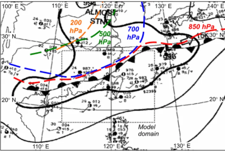
Figure 1.CWB surface analyses and positions of front/trough (or wind-shift line, thick dashed) at 850 (red), 700 (blue), 500 (green), and 200 hPa (orange) at 12:00 UTC on 11 June 2012. The CReSS model domain is marked by the dotted box.

resolution (or (1/120)◦, roughly 900 m) and observed weekly sea surface temperature (Reynolds et al., 2002) are provided. The model configuration and major aspects of the experiment are summarized in Table 1.

2.3 Analysis of vertical momentum and pressure perturbations

To investigate the BB process taking place in the present case using model outputs, the methods below, following Wil-helmson and Ogura (1972), Rotunno and Klemp (1982), Klemp (1987), and Parker and Johnson (2004), are used to perform analysis of vertical momentum and pressure pertur-bations. With the background environment assumed to be in hydrostatic equilibrium, the vertical momentum equation can be written as

dw

dt = −

1

ρ ∂p′

∂z −

ρ′

ρ g+Fz≈ −

1

ρ0 ∂p′

∂z −

ρ′ ρ0

g+Fz, (1)

where all variables have their conventional meanings. Here,

ρ=ρ0+ρ′, whereρ0is the background value andρ′the

per-turbation part ofρ,B= −g(ρ′/ρ0)is the buoyancy, andFz

is the friction term by turbulent mixing. Thus, the vertical ac-celeration is driven by an imbalance among the perturbation PGF, buoyancy, and turbulent mixing. The buoyancy is con-stituted by the gaseous effect and the drag of all condensates, and can be expressed as

B= −ρ

′

ρ0

g=gθ

′ v θv0

−gXqx, (2)

whereθvis the virtual potential temperature (andθv=θv0+ θ_v′) and its perturbation accounts for the gaseous effect, while

qxdenotes the mixing ratio of any condensate species.

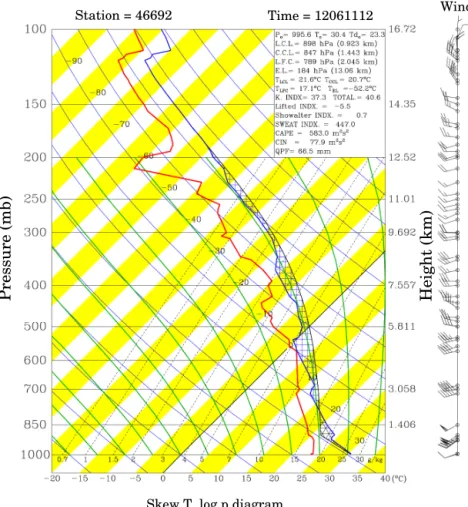
Table 1.The CReSS model domain configuration and physics used in this study.

Projection Lambert conformal (center at 120◦E, secant at 10 and 40◦N)

Grid spacing 1.5 km×1.5 km×100–980 m (400 m)∗

Dimension and size (x,y,z) 1000×800×50 (1500 km×1200 km×20 km)

IC/BCs NCEP 0.5◦×0.5◦analyses (26 levels, every 6 h)

Topography and sea surface temperature Real at (1/120)◦and weekly mean on 1◦×1◦grid

Integration period 12:00 UTC on 10 June to 12:00 UTC on 12 June 2012 (48 h)

Output frequency Every 15 min (every 5 min during 18:00–24:00 UTC on 11 June)

Cloud microphysics Bulk cold-rain scheme (6 species)

Planetary boundary layer parameterization 1.5-order closure with prediction of turbulent kinetic energy

Surface processes Energy/momentum fluxes, shortwave and longwave radiation

Substrate soil model 41 levels, every 5 cm to 2 m deep

∗_{The vertical grid spacing (1z) of CReSS is stretched (smallest at the bottom), and the averaged spacing is given in the parentheses.}

omitted (e.g., Rotunno and Klemp, 1982; Parker and John-son, 2004), are

∇2p′_b= ∂

∂z(ρ0B) , (3)

and

∇2p′_d= −ρ0

"

∂u ∂x

2

+

_∂v

∂y

2

+

_∂w

∂z

2

−w2∂

2

∂z2(lnρ0)

−2ρ0

_∂v

∂x ∂u

∂y+

∂u ∂z

∂w ∂x

+∂v

∂z ∂w

∂y

, (4)

where∇2is the Laplacian operator. In both equations, a pos-itive (negative) center in ∇2p′ corresponds to a local min-imum (maxmin-imum) inp′itself. Equation (3) states thatp′_bis related to the vertical gradient of the product ofρ0andB. On

the right-hand side of Eq. (4), inside the brackets are exten-sion terms which imply maximizedp_d′ in regions of nonzero divergence or deformation. The other terms inside the paren-theses are shearing terms and imply minimizedp_d′ in regions of nonzero vorticity (Parker and Johnson, 2004). The shear-ing effects include those related to vertical wind shear (∂u/∂z

and∂v/∂z) associated with the LLJ, as reviewed in Sect. 1

for the Morakot case. After∇2p_b′ or∇2p′_dis obtained from Eqs. (3) or (4), the relaxation method is used to solve the associated pressure perturbation through iteration (see Ap-pendix A for details).

To provide additional verification, a second, independent method is also used in this study to computep′as in WKJ15. In this method,p′is separated from its background pressure (p0), defined as

p0(x, y, z, t )= hpi(x, y, z)+1p(z, t ), (5)

wherehpiis the time-averaged pressure over a fixed period, and1pis the deviation of the areal-mean pressurepat any given instant from its time meanhpi, such that

1p(z, t )=p(z, t )− hpi(z). (6)

Thus, the gradual decrease of the areal-mean pressure with time as the meiyu front approaches from the north is reflected in1pand taken into account inp0besides the spatial

varia-tion in (time-averaged) meanp(cf. Eq. 5). Then,p′is com-puted simply as

p′(x, y, z, t )=p(x, y, z, t )−p0(x, y, z, t ). (7)

Referred to as the separation method, it is also applied to other variables to separate the perturbation and the back-ground where needed, such as forρ andθv in Eqs. (1) and

(2), as well as potential temperatureθ and horizontal wind componentsuandv.

3 Case overview

3.1 Synoptic and storm environment

(e) 6/11 13 Z (f) 6/12 02 Z

(a) (b)

6/11 12 Z 6/11 12 Z

(d) (c)



6/11 06Z 12Z 18Z

6/12 00Z 06Z 12Z

6/11 06Z 12Z 18Z

6/12 00Z 06Z 12Z

116º E 118º E 120º E 122º E 124º E 27º N

26º N

25º N

24º N

23º N

22º N

21º N

20º N

27º N

26º N

25º N

24º N

23º N

22º N

21º N

20º N

116º E 118º E 120º E 122º E 124º E

27º N

26º N

25º N

24º N

23º N

22º N

21º N

116º E 118º E 120º E 122º E 124º E 27º N

26º N

25º N

24º N

23º N

22º N

21º N

116º E 118º E 120º E 122º E 124º E

116º E 118º E 120º E 122º E 124º E 116º E 118º E 120º E 122º E 124º E 26º N

24º N

22º N

26º N

24º N

22º N

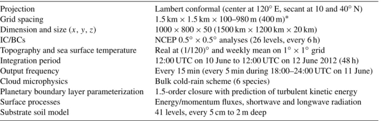
Figure 2. (a) NCEP (0.5◦) 950 hPa analysis and(b)CReSS simulation of horizontal winds (m s−1, speed shaded, scale to the right) at z=549 m at 12:00 UTC on 11 June 2012, with frontal position marked (thick dashed lines).(c, d)Frontal positions every 6 h from 06:00 UTC on 11 June to 12:00 UTC on 12 June 2012(c)at 950 hPa in NCEP analyses and(d)atz=549 m in model (see legend for line color and style), overlaid with topography (km, shading, scale to the right). The triangle in panel(c)marks the location of Panchiao sounding in Fig. 3.

(e, f)ASCAT oceanic winds (m s−1) near Taiwan at(e)13:00 UTC on 11 June and(f)02:00 UTC on 12 June 2012, with surface frontal position analyzed.

to flow splitting due to terrain blocking and the subsequent channeling, confluence, and acceleration, with local wind maxima, i.e., barrier jets, near the two ends of Taiwan (e.g., Li and Chen, 1998; Wang ad Chen, 2002; Chen et al., 2005). For the one in northern Taiwan Strait (Fig. 2a), in particu-lar, the low-level convergence (from confluence) associated with the barrier jet can provide the forcing for quasi-linear MCSs near or south of the front (e.g., Yeh and Chen, 2002; Wang et al., 2005). The NCEP analyses every 6 h shows that the 950 hPa front reached northern Taiwan near 00:00 UTC on 12 June (Fig. 2c), also consistent with ASCAT data at

02:00 UTC (Fig. 2f). Afterward, as the rainfall in northern Taiwan gradually weakened (cf. Figs. 4 and 9, to be discussed later), the meiyu front advanced rapidly across Taiwan and reached about 23◦N within 6 h (Fig. 2c).

pro-Pressure (mb) Height (km)

Skew T, log p diagram

Station = 46692 Time = 12061112 Wind

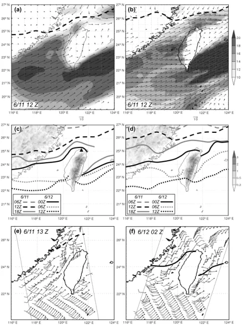
Figure 3.Thermodynamic (skewT-logp) diagram for the sounding taken at Panchiao (46 692, cf. Fig. 2c for location) at 12:00 UTC on 11 June 2012. For winds, full (half) barbs denote 10 (5) kts (1 kt=0.5144 m s−1).

file, while that further aloft was less steep but still mostly exceeded the moist adiabat, indicating conditional instability up to about 550 hPa. The convective available potential en-ergy (CAPE) was 583 J kg−1and sufficient to support deep convection if the air parcel could overcome the convective inhibition (CIN) of 78 J kg−1to reach the level of free con-vection at 789 hPa. Obviously, these conditions were soon met since heavy rainfall did occur in Taipei. Note also that the humidity was quite high below about 550 hPa, and a dry layer did not exist throughout the troposphere. Thus, with instability and low-level convergence, the strong, deep, and moisture-laden southwesterly flow near and to the south of the approaching meiyu front was clearly very favorable for active convection and substantial rainfall (e.g., Jou and Deng, 1992; C.-C. Wang et al., 2014a).

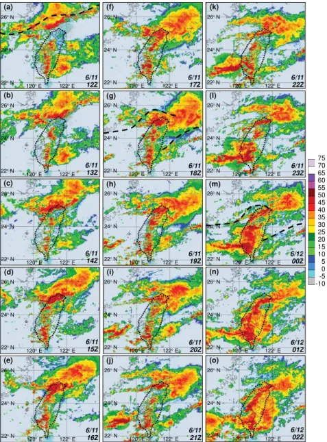
3.2 The back-building rainband with extreme rainfall Figure 4 presents the composite VMI radar reflectivity from the ground-based radars in Taiwan at 1 h intervals and depicts the evolution of the rainbands causing the extreme rainfall in northern Taiwan. At 12:00 UTC on 11 June (Fig. 4a), an

Tai-75 70 65 60 55 50 45 40 35 30 25 20 15 10 5 0 -5 -10

24

26

120

22

122

24

26

120

22

122

24

26

120

22

122 6/11

15Z

6/11 20Z

6/12 01Z

(d) (i) (n)

24

26

120

22

122

24

26

120

22 _122

24

26

120

22 _122

6/11 16Z

6/11 21Z

6/12 02Z

(e) (j) (o)

(a)

24N 26

120

22

122

24

26

120

22 _122

24

26

120

22 _122

6/11 12Z

6/11 17Z

6/11 22Z

(f) (k)

24

26

120

22

122

24

26

120

22

122

24

26

120

22

122 6/11

14Z

6/11 19Z

6/12 00Z

(c) (h) (m)

24

26

120

22

122

24

26

120

22

122

24

26

120

22

122 6/11

13Z

6/11 18Z

6/11 23Z

(b) (g) (l)

N

E N

E

N N

E N

E

N N

E N

E

N N

E N

E

N N

E N

E

N N

E N

E

N N

E N

E

N N

E N

E

N N

E N

E

N N

E N

E

N N

E N

E

N N

E N

E

N N

E N

E

N N

E N

E

N N

E N

E

Figure 4.Composite VMI radar reflectivity (dBZ, color, scale to the right) over the Taiwan area at 1 h intervals from(a)12:00 UTC on 11 June to(i)02:00 UTC on 12 June 2012. The outline of Taiwan is highlighted (thick dotted lines) and the surface frontal position is plotted at synoptic times (thick dashed lines).

wan also received continuous rainfall from forced uplift of the strong LLJ by the topography (cf. Fig. 2a and c), and an-other squall line also approached southern Taiwan from the west and made landfall near 22:00 UTC on 11 June (Fig. 4i– o). Nonetheless, the reflectivity over northern Taiwan was both very active and lengthy, and was produced by two types of MCSs: the first was the squall line before 18:00 UTC on 11 June and reminiscent to a TL/AS system, and the second was the quasistationary BB MCS after 18:00 UTC (Fig. 4).

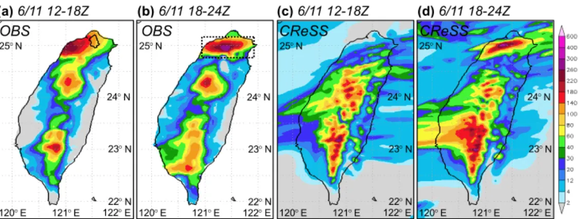
The distributions of 6 h accumulated rainfall during 12:00–18:00 and 18:00–24:00 UTC on 11 June are shown in Fig. 5a and b. While three distinct rainfall centers over north-ern, central, and southern Taiwan were produced in each pe-riod, the amount over northern Taiwan was the highest. The

120 E N 25

(a)6/11 12-18Z

OBS

121

N

(b)6/11 18-24Z (c)6/11 12-18Z (d)6/11 18-24Z

OBS CReSS CReSS

120 E

N 25

121

N

120 E

N 25

121

N

120 E

N 25

121

N

N N N N

E N

E E

N

E E

N

E E

N

E 122

24

23

22

122 24

23

22

122 24

23

22

122 24

23

22

Figure 5.Distribution of observed 6 h accumulated rainfall (mm, color, scale to the right) over Taiwan during(a)12:00–18:00 UTC and

(b)18:00–24:00 UTC on 11 June 2012. The Taipei City boundary is depicted in panel(a), and the dotted box in panel(b)shows the region used in Fig. 8 for rainfall average.(c, d)As in panels(a, b), but showing model-simulated rainfall over Taiwan and the surrounding oceans.

While back-building likely also occurred in the TL/AS-type squall line, such behaviors in the quasistationary rain-band after 18:00 were well depicted by the radar VMI reflec-tivity every 10 min (Fig. 6). As marked by the short arrows, frequent BB activities can be spotted at the western end of the convective line or west of existing mature cells, and some of them were quite close to the northwestern coast of Tai-wan. After formation, they moved at small angles from the ENE–WSW-oriented quasistationary line, repeatedly across northern Taiwan with frequent cell mergers similar to those in WKJ15 (Fig. 6). The resulted rainfall in Fig. 5b, with the maximum located inland near Taipei, also implies that many cells matured after they moved onshore instead of over the ocean prior to landfall. Since the length of the line with ac-tive cells upstream from Taipei is about 160 km and most cells traveled at the speed range of 60–80 km h−1in Fig. 6, the heavy rainfall would last only 2–2.5 h and much shorter than in reality (cf. Fig. 5) if there were no new developments westward along the line.

In extreme events, there are often multiple factors of dif-ferent scales working in synergy to lead to their occurrence. This is also true in the present case, and the scenario leading to heavy rainfall can be quite complicated. While the large and synoptic-scale conditions provided a favorable back-ground (Figs. 1–3), the two MCSs developed south of the approaching meiyu front, in close proximity to the area of terrain-influenced low-level convergence (and the barrier jet) near northern Taiwan (Figs. 2a, c, e, and f, and 4). In Figs. 4 and 6, the convective lines even exhibited characteristics of multiple lines at times, possibly linked to gravity-wave ac-tivities (e.g., Yang and Houze, 1995; Fovell et al., 2006). While the formation mechanism of the quasi-linear MCSs (the second one in specific) and the roles played by both the meiyu front and the topography will be discussed and clari-fied (Sect. 4.2), the BB process at the convective scale was also a contributing factor to the extreme rainfall, especially during the later 6 h period after 18:00 UTC (Fig. 6). Also, as

typical in many events, the new BB cell is often found to de-velop about 15–30 km upstream from an old cell in Fig. 6. Thus, why this particular spot has an advantage for new cell initiation compared to other locations without a nearby old cell is the scientific question that we wish to answer and the main focus of this case study. This specific question (and the formation mechanism of the MCSs) will be addressed through our numerical simulation results below.

4 Results of model simulation 4.1 Model result validation

As described in Sect. 2.2, our CReSS model simulation was performed from 12:00 UTC on 10 June 2012 for 48 h us-ing NCEP (0.5◦) final analyses as IC/BCs, with a horizontal grid spacing of 1.5 km. The simulated winds and the front at an elevation of 549 m (close to 950 hPa) at 12:00 UTC on 11 June (t=24 h) and frontal positions every 6 h are shown in Fig. 2b and d. Compared to the observation and NCEP analyses (Figs. 1, 2a, and e), the simulated front in Fig. 2b is slightly too north, especially west of 120.5◦E and over land in southeastern China, but the prefrontal LLJ is well captured, including the strong winds (barrier jet) near northern Taiwan. Linked to the position error of the front at 12:00 UTC, the modeled front is also too north at 18:00 UTC, but its western segment over the strait advanced southward more rapidly to catch up with the NCEP analyses during the next 6 h (Fig. 2c and d). The segment east of Taiwan, how-ever, is still too north at 00:00 UTC, 12 June (cf. Fig. 2f), and the position error there does not improve until about 12 h later (Fig. 2c and d).

24 120

1940Z

(a)

24 120

1950Z

(b)

24 120

2000Z

(c)

24 120

2010Z

(d)

24 120

2020Z

(e)

24 120

2030Z

(f)

24 120

2040Z

(g)

24 120

2050Z

(h)

24N 120E

2100Z

(i)

24 120

2110Z

(j)

24 120

2120Z

(k)

24 120

2130Z

(l)

24 120

2140Z

(m)

24 120

2150Z

(n)

120

2200Z

(o)

24

75 70 65 60 55 50 45 40 35 30 25 20 15 10 5 0 -5 -10

N E

N E

N E

N E

N E

N E

N E

N E

N E

N E

N E

N E

N E

E N

Figure 6. As in Fig. 4, but showing reflectivity over northern Taiwan and the upstream area every 10 min from (a) 19:40 UTC to

(o)22:00 UTC on 11 June 2012 using a different set of colors. The arrows mark the initiation or strengthening of back-building cells, off the western end of a rainband or upstream from an old cell.

to the north of the near-surface front (Fig. 7a–d) and differ-ent from the training-line system ahead of the front in the observation. Thus, the simulation of the first MCS was not ideal in location, apparently linked to the frontal position er-ror discussed earlier. However, the quasistationary MCS over northern Taiwan since 18:00 UTC, with intense convective cells near Taipei, and the second squall line over the south-ern strait are both nicely captured in the model as the front advanced south (Fig. 7d–f). As a result, the rainfall simu-lation in northern Taiwan during 18:00–24:00 UTC, with a peak amount of 312 mm, is in close agreement with the ob-servation (Fig. 5b and d), while that during the preceding 6 h was not (Fig. 5a and c). Similar results are also revealed by hourly histogram of rainfall in Fig. 8, averaged inside the elongated box depicted in Fig. 5b. The rainfall in northern Taiwan was much better simulated in magnitude and varia-tion in time after 18:00 UTC, 11 June (Fig. 8), although the areal-averaged intensity in the model is somewhat lower be-cause the simulated rain belt is narrower than the one ob-served (Fig. 5b and d). Also, the model predicted more rain-fall than observed over the mountains in southern Taiwan (Fig. 5), indicating that the flow over the terrain might be somewhat overestimated, though this is not our focus here. 4.2 Formation of the quasi-linear MCS

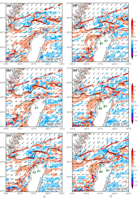
The more detailed distributions of horizontal winds and con-vergence/divergence near the surface at 312 m from 18:30 to 21:00 UTC on 11 June 2012 in the model are shown in Fig. 9. With a wavy pattern and strong convergence along most of its

length, the near-surface meiyu front (black dotted curves) is north of Taiwan but gradually approaches during this period. Consistent with Figs. 1, 2, 6, and 7, the quasi-linear and sta-tionary MCSs, in contrast, developed south of the front near 25◦_{N. As the front advances, their distance decreased from}

about 90 km at 18:30 UTC to 30 km at 21:00 UTC (Fig. 9), and in the observation the front only caught up with the pre-frontal MCS after 00:00 UTC on 12 June as mentioned (cf. Figs. 2c and 4g–o). Crossing northern Taiwan, the rainband forms along a near-surface convergence zone (green dotted curves, mostly > 5×10−5s−1with confluence and accelera-tion) between the flow blocked and deflected northward by the topography of Taiwan and the unblocked flow farther to the north and west in the environment (but still ahead of the front, Fig. 9). Thus, in agreement with the observations, the effects of terrain (blocking) appeared to play a key role to initiate the rainband development, while the front helped provide and channel an enhanced background flow with its approach in the present case. Such a scenario is quite sim-ilar to those studied by Yeh and Chen (2002) and Wang et al. (2005). Thus, the frontal forcing, LLJ, terrain effects, and the BB process all work together to lead to the quasi-linear MCS and heavy rainfall in northern Taiwan in the present case. However, it is not possible to isolate and quantify their individual contribution here, and we do not intend to do so.

(b) (e)

1400 UTC 2000 UTC

(c) (f)

1600 UTC 2200 UTC

(a) (d)

1200 UTC 1800 UTC

27º N

26º N

25º N

24º N

23º N

22º N

27º N

26º N

25º N

24º N

23º N

22º N

27º N

26º N

25º N

24º N

23º N

22º N

27º N

26º N

25º N

24º N

23º N

22º N

27º N

26º N

25º N

24º N

23º N

22º N

27º N

26º N

25º N

24º N

23º N

22º N

118º E 119º E 120º E 121º E 122º E 123º E 124º E 118º E 119º E 120º E 121º E 122º E 123º E 124º E

118º E 119º E 120º E 121º E 122º E 123º E 124º E 118º E 119º E 120º E 121º E 122º E 123º E 124º E

118º E 119º E 120º E 121º E 122º E 123º E 124º E 118º E 119º E 120º E 121º E 122º E 123º E 124º E

Figure 7.CReSS simulation of surface winds at 10 m height (m s−1) and column-maximum mixing ratio of precipitation (rain+snow + graupel, g kg−1, shading, scale to the right) every 2 h from(a)12:00 UTC to(f)22:00 UTC on 11 June 2012. For winds, full (half) barbs denote 10 (5) m s−1, and the surface frontal positions are marked (thick dashed lines). The rectangle in panel(a)depicts the area (24.75–25.15◦N, 120.35–121.75◦E) used for the separation method.

labeled as “A2” develops about 20 km upstream from the old cell “A1” around 19:30 UTC and becomes mature near 20:10 UTC. Likewise, “B2” is triggered west of “B1” after 21:20 UTC and develops into a mature cell near 21:40 UTC and then the two cells merge near 21:50 UTC over northern Taiwan (Fig. 10, also cf. Fig. 9), in a way similar to that discussed by WKJ15. In the model, the training of

se-11 Jun 12 Jun

Date and time (UTC)

H

ou

rly

ra

in

fa

ll

(m

m

) Obs CReSS

Figure 8.Time series of observed (gray bars) and simulated (curve with dots) hourly rainfall (mm), averaged inside the box shown in Fig. 5b (24.75–25.17◦N, 120.87–121.85◦E) over northern Taiwan from 12:00 UTC on 11 June to 06:00 UTC on 12 June 2012.

lected for the separation ofp0andp′, as described at the end

of Sect. 2.3, are set to 24.75–25.15◦N, 120.35–121.75◦E (cf. Fig. 7a) and over 18:00–24:00 UTC on 11 June 2012. 4.3 Structure of convective cells in the BB MCS In this subsection, the simulated structure of convective cells inside the BB system is first examined, before the discussion on the finer details of pressure perturbations and their associ-ated effects in the BB process. The pair of old and new cells for study has been chosen to be B1 and B2 over the period of 20:00–21:40 UTC, as they are farther away and less affected by the terrain of northern Taiwan (cf. Fig. 10). To reveal the storm environment (provided by the background forcing), E–W vertical cross sections along 25◦_{N through the}

cen-ters of both B1 and B2 (line AB in Fig. 10) are constructed and averaged over three outputs from 21:25 to 21:35 UTC, as shown in Fig. 11a. The equivalent potential temperature (θe) has a minimum of about 350 K at mid-levels (near 4–

5 km) and increases both upward and downward in upstream as well as downstream regions, indicating the presence of convective (and conditional) instability (cf. Fig. 3). During the average period, the mean updraft of B1 is located near 121.35◦E (cf. Fig. 10), and its immediate upstream region, i.e., where cell B2 is developing (∼121.2◦E), is character-ized by strong near-surface convergence coupled with upper-level divergence (Fig. 11a). Clearly favorable for new cell development upstream with near-surface convergence there, such a thermodynamic and kinematic structure under the in-fluences of the front and terrain (as discussed in Sect. 4.2) is very similar to the composites of BB MCSs in the USA obtained by Schumacher and Johnson (2005, their Fig. 17b). The WSW–ENE cross section (along low-level flow) through B1 about 30 min earlier at 21:00 UTC shows a gradual ac-celeration of the upstream LLJ (thick arrow line) under the forcing of background convergence. As the jet approaches B1, which is already in mature stage (and quasi-steady),

there is a rapid local acceleration then intense deceleration across B1, by about 10 m s−1with a convergence in excess of 5×10−3s−1 (Fig. 11b). While this local acceleration is clearly a response to the development of B1, the resulting vertical wind shear from the south-southwest is strongest be-low 500 m under B1 and its immediate upstream, where a value of about 2–3×10−2s−1can be reached (Fig. 11c). The vertical wind shear upstream from B1 further aloft turns into northerly and then northeasterly at about 2 km, as expected above the axis of the LLJ, but its value (∼3×10−3s−1) is 1 order of magnitude smaller (Fig. 11c). Thus, the verti-cal wind shear in the storm environment of B1 (and B2) is strongest near the surface. Also, the deep convection can be seen to tilt eastward with height in both cross sections, con-sistent with the direction of the upper-level winds and the evolution of stratiform area (cf. Figs. 3 and 4).

In Fig. 12, the perturbations inθ (i.e.,θ′) and horizontal winds (u′ _{and v}′_{) obtained through the separation method}

(cf. Sect. 2.3), as well as the associated convergence and divergence, surrounding the pair of cells B1 and B2 at the surface between 20:00 and 21:00 UTC are presented every 20 min. During this initiation period of B2, while there ex-ists positive θ′ (of 0.4–0.8 K) below the updraft of B1, its induced cold pool is very weak at the surface, with aθ′ of only−0.3 K at most, and is roughly 10 km to the east at the forward flank (Fig. 12). The convergence at the leading edge of the diverging, marginally colder air (denoted by dotted curves) extends to the southeast and south of B1 at 20:00– 20:20 UTC (Fig. 12a and b) but gradually moves to the east afterwards (Fig. 12c and d). At the rear side of B1, the new cell B2 (marked by a blue “x”) develops inside a region of surface convergence, consistent with Fig. 9d, e, and f, and quite far (at least 10 km) from both the weak cold pool and the leading edge of its outflow (Fig. 12). Therefore, the cold pool does not play any significant role in the initiation of the back-building cell B2 in the model, and the B1–B2 pair ap-pears to be ideal for further investigation in greater detail.

The results of∇2p′ obtained by the two different meth-ods (by separation and from Eqs. 3 and 4) as described in Sect. 2.3 at two different heights near 0.8 and 3 km are com-pared in Fig. 13, also for 21:00 UTC as an example. In gen-eral, the patterns are very similar. At 0.8 km, negative∇2p′

(implyingp′> 0) occurs near the updraft of B1 with posi-tive∇2p′ (implying p′< 0) to the east near the downdraft (Fig. 13a and b). West of B1, where B2 is developing, posi-tive (negaposi-tive)∇2p′is found to the south (north) of the near-surface convergence zone. Near 3 km, the updraft of B1 cor-responds to∇2p′_{> 0 and∇}2_p′_{< 0 occurs to its western flank}

(a) (d)

1830 UTC 2000 UTC

(b) (e)

1900 UTC 2030 UTC

(c) (f)

1930 UTC 2100 UTC

B1 B2 C1 A1

A2 A1

B2 B1 B1 A2

119º E 120º E 121º E 122º E 123º E

27º N

26º N

23º N 24º N 25º N

119º E 120º E 121º E 122º E 123º E

27º N

26º N

24º N 25º N

119º E 120º E 121º E 122º E 123º E

27º N

26º N

23º N 24º N 25º N

119º E 120º E 121º E 122º E 123º E

27º N

26º N

24º N 25º N

119º E 120º E 121º E 122º E 123º E

27º N

26º N

23º N 24º N 25º N

119º E 120º E 121º E 122º E 123º E

27º N

26º N

24º N 25º N

Figure 9.CReSS simulation of horizontal winds (m s−1, vectors, reference length at bottom) and convergence/divergence (10−4s−1, shad-ing, scale to the right, positive for convergence) at 312 m height (contoured in thick gray) every 30 min from(a)18:30 UTC to(f)21:00 UTC on 11 June 2012. The frontal positions (black dotted lines) and convergence axis (green dotted lines) and convective cells of interests are marked.

4.4 Analysis of pressure perturbations

To examine the distributions of pressure perturbations and their roles in the BB process in greater detail, a series of ver-tical cross sections through the updraft center of B1 at 5 km and the near-surface center of B2 from 20:00 to 21:00 UTC (each roughly 50 km in length, cf. Figs. 10 and 12), i.e.,

120.5 E 121.0E 121.5E

2120 UTC

2130 UTC

2140 UTC

2150 UTC

2200 UTC

2210 UTC

B2 B1 C1

B2 C1

C1

B2

B2 C1

B2 C1

B2 C1

A B

120.5E

25.0N

121.0E

1920 UTC

1930 UTC

1940 UTC

1950 UTC

2000 UTC

2010 UTC

121.5E

25.0N

25.0N

25.0N

25.0N

25.0N

A1 A2

A2

A1 A2

A2

A2

A2 B1

B1

120.5E 121.0E 121.5E

2020 UTC

2030 UTC

2040 UTC

2050 UTC

2100 UTC

2110 UTC B2 B1

B2

B2 B1 C1

C1 C

D B1

B1 B1



Figure 10.Model-simulated column-maximum vertical velocity (w, m s−1, color and thin contours) every 10 min during 19:20–22:10 UTC on 11 June 2012, overlaid with terrain elevation (m, thick contours at 250 and 500 m) in northern Taiwan. The color scale is shown at the bottom, and the contour at 0.5 m s−1is not drawn. Old cells (A1, B1, and C1) and nearby new cells (A2, B2) of interests are labeled. Green dashed lines AB and CD depict the vertical cross sections used in Fig. 11, and the short segments depict those used in Figs. 14–18 (blue (brown) ones through B1 (C1)).

120.6

(a)6/11 2125-2135 UTC

120.9 121.2 121.5  121.8

A B

9

8

7

6

5

4

3

2

1

H

ei

gh

t (

km)

354

356 356

356

356 358

354 352

354

356 ₃₅₂

354 356 358 360

358 354

352

352

356

362

352

(c)6/11 2100 UTC

B1 5.0

4.5 4.0 3.5 3.0 2.5 2.0 1.5 1.0 0.5 0.0

120.6C 120.9 121.2 121.5 D

8 5 2 1 0.5 0.5 1 2 5 8 5

H

ei

gh

t (

km)

(b)6/11 2100 UTC

5.0 4.5 4.0 3.5 3.0 2.5 2.0 1.5 1.0 0.5 0.0

11 12

12 12

12 11 10

15 14

15

15 16 16 14 13

16 19 19

20 13 13

17 18 9

8 10

120.6C 120.9 121.2 121.5

30 20 10 5 2 2 5 10 20 30 10 D

E E E E E

E E E E E E E E

Figure 11. (a)E–W vertical cross section of model-simulated convergence/divergence (10−4s−1, color, positive for convergence) andθe(K,

(a)2000 UTC

(b)2020 UTC

(c)2040 UTC

(d)2100 UTC B1

B2

B1

B2 x

B2

B1

x

B1 x

25º N

24.8º N

24.6º N

120.6º E 120.8º E 121º E 121.2º E

25º N

24.8º N

24.6º N

120.6º E 120.8º E 121º E 121.2º E

25º N

24.8º N

24.6º N

120.6º E 120.8º E 121º E 121.2º E

25º N

24.8º N

24.6º N

120.6º E 120.8º E 121º E 121.2º E

Figure 12.CReSS simulation of convergence/divergence (10−4s−1, shading, scale to the right, positive for convergence), 10 m wind per-turbation (m s−1, green vectors, reference length at bottom), and potential temperature perturbation (θ′, K, contours every 0.1 K, dashed for negative values) at the surface every 20 min from(a)20:00 UTC to(f)21:00 UTC, 11 June 2012. Cells B1 (black) and B2 (blue), axis of convergence (thick dotted line) produced by downdraft outflow of B1, and locations of vertical cross sections as in Fig. 10 (straight dashed lines) are marked.

mid-level and negative both above and below, corresponding top′< 0 andp′> 0, respectively (as labeled by “L” and “H”). Again, the pattern of∇2p′is largely attributable to its buoy-ant (∇2p_b′) instead of dynamical component (∇2p′_d, Fig. 14b and c). Twenty minutes later at 20:20 UTC (Fig. 14d), the updraft of B1 strengthens to more than 8 m s−1 and be-comes more tilted, but the basic pattern of∇2p′at its west-ern flank and the upstream region remains. At this time, the suppressing downdraft there weakens, and B2 is develop-ing (∼0.5 m s−1) just west of the sinking motion and about 15 km upstream from the core of B1. This new development is associated withp′< 0 below 1 km andp′> 0 over 1–3 km, and the perturbations (and those of B1) are also mainly from the buoyant rather than dynamical effects (Fig. 14e and f).

At 20:40 UTC (Fig. 14g), B1 further strengthens and is even more tilted with height, and its associated downdraft below the mid-level (> 2 m s−1near 4 km) now appears only at the eastern (downwind) side (cf. Fig. 12c). The upward motion of B2 can now reach over 1 m s−1and extend further upstream, while a layer of positive ∇2p′ (implying p′< 0) forms near 5 km, again mainly from the buoyant effects (cf. Fig. 14h). The distribution of∇2p′_dis only significant at both flanks of the updraft of B1 below about 3.5 km (and at its eastern flank near 5 km, Fig. 14i), which forms gradually as

B1 intensifies (Fig. 14c and f). The configuration of posi-tive (negaposi-tive)p′_dat the rear (forward) flank of the updraft near 500 mm (below the jet level, cf. Fig. 11c) and a reversed pattern above (near 2–3 km) is consistent with the shearing (plus extension) effect (cf. Eq. 4), in agreement with WKJ15 and other earlier studies. However, sincewand its horizontal gradient are weak near the surface, where the vertical wind shear is larger (also Fig. 11c), the value of∇2p_d′ is smaller than that in WKJ15. Also, due to the farther distance, a direct role played by the dynamical pressure perturbations in new cell initiation of B2 appears limited in the present case here. Both B1 and B2 intensify at 21:00 UTC, and the latter, peaking at about 1.5 m s−1, can now reach 4 km while the layer of ∇2p′> 0 above (near 5 km) also grows stronger (Fig. 14j). A downdraft at the rear flank of B1 reappears at mid-levels and penetrates down to 3 km at this time, acting to separate B2 from B1 (also Fig. 13d). Like earlier times since 20:20 UTC, the total pattern of∇2p is dominated by

conver-121.0E

(a)

120.9E 121.1E 121.2E N N N N N 121.0E (b)

120.9E 121.1E 121.2E N N N N N 121.0E (c)

120.9E 121.1E 121.2E N N N N N (d) 121.0E

120.9E 121.1E 121.2E

(e)

121.0E

120.9E 121.1E 121.2E

(f)

121.0E

120.9E 121.1E 121.2E B1 B2 B1 B2       

-6 _-6 -6 _-6

-3 -3 -9 -6 -9 3 3 3 -3 6 6 6

3 33 33 30 -3 -12 -12

-27

-9 -3

18 15 12 9 9

24

-3 -3

-6 -9 _-3

-6 21 -3 -6 24 18 9 9

12 9 12 -9 -9 -3 6 3 -6 -3 -3 12 -3

-6 -6 -9 -6

-3 _-9 -6 -3 -12 -18 -21 -24 -3

3 6 9 18 15

3 -6 -3 -6 -6 -9 3 6

30 36 ₃₃ 33 -3 30 -6 -9 -30 -12 -3 -12 6 -18 18 24 -6 6 3 3 3 -3 -6

-6 3

-3

9 12 15 12 15 24 21

15 12 _{9 9} -3 -3 -12 3 6 -3 -6 -9

3 3 -3

-3 -6

-6 -9

-12 -18 6 6

9 15 9 12 3 -21 -3 -6 -6 -9 -3 -15

12 6 -3 -9

27 33 36 -18 -21 -6 18 -6 6

30 24 3

-12

-9 _-3

-3 -3 -3 3 3 3 18 15 -6 -9

-12

15 9 6 126 -12 -3 15 12 9 3 3 -3 -6 24.88 24.92 24.96 24.84 25.00 24.88 24.92 24.96 24.84 25.00 24.88 24.92 24.96 24.84 25.00

Figure 13.Model-simulatedw(m s−1, color, scale at bottom) and Laplacian of perturbation pressure (10−6Pa m−2, contour, every 3× 10−6Pa m−2, dashed for negative values) of cells B1 and B2 at (left) 806 m and (right) 2929 m at 21:00 UTC on 11 June 2012.(a, d)∇2p′ obtained from separation method;(b, e)∇2p′= ∇2p′_b+ ∇2p_d′ and(c, f)∇2p′_bcomputed from Eqs. (3) and (4). Cells B1 and B2 and updraft and downdraft centers are labeled in panels(a)and(d).

gence in driving the development of the line-shaped MCS in this event, as also shown earlier in Sect. 4.2 (and cf. Fig. 11a). Nevertheless, the propagation speed of B1 is indeed slower than B2 in Fig. 10 and can be estimated to be about 8.9 m s−1 near 21:00 UTC. Caused by the dynamical effect ofp′_d, this slowdown implies an increase in low-level blocking and sub-sequent upstream convergence by about 1×10−4s−1 us-ing Fig. 11b (with a LLJ of 12.5 m s−1 near 40 km up-stream), or 2.2×10−4s−1 larger than its surrounding with a background speed divergence of∼1.2×10−4s−1 follow-ing WKJ15 (p. 11109). Since this is no more than 20 % of the maximum convergence near B2 and its immediate upstream (west of 121.2◦E, cf. Fig. 11a), the minor role ofp_d′ in the initiation of B2 in the present case can be confirmed.

The buoyancyB (or more precisely, the vertical buoyant force per unit mass) in Eq. (1) and its contributing terms as given in Eq. (2) on the same vertical cross sections are shown in Fig. 15. At 20:00 UTC, as expected, B is posi-tive inside the cumulonimbus B1 and negaposi-tive in the top portion of the cloud (> 6.5 km) and below the main updraft (< 2 km, Fig. 15a). Such a pattern is due to the combined effects of positive virtual potential temperature perturbation ( θ_v′> 0) clearly from latent heat release (LHR) inside the cloud and the downward drag by all hydrometeors

(includ-ing both cloud particles and precipitation) maximized below the updraft core (Fig. 15b and c). In the downdrafts at the flanks (which originate from higher levels),Bandg(θ_v′/θv0)

are also mostly positive from adiabatic warming outside the cloud.

H H L L L H H L L L L L H H ei gh t ( km ) 8 7 6 5 4 3 2 1 0

(a)2_{p’ 2000 UTC (b)}2_p’

b 2000 UTC (c)2p’d 2000 UTC

-27

21 15 -6

15

12 30 21 24 15 18 3 18 -3 -3

-3 -3 -3 -9 -12 -24

3

3 3 6 3

6 -12

21 _{9 -3} -6 3 6

9 12 15 18

18 ₂₁ 15 3 3 3 6 -3 -12 -18

-24 -27

-15 -12 3 -3

-3 -9 -9 -6 -6

-3 3 6

12 ₂₁ 24

18 15 -6

-3 -3 -3 3 3 3 6 9 9 6 3 6 H H L L

L H

H L L L L L H H

L L

H L H ei gh t ( km ) 8 7 6 5 4 3 2 1 0

(d)2_{p’ 2020 UTC (e)}2_p’

b 2020 UTC (f)2p’d 2020 UTC

-3 -3 -3 -6 -9 -3 -3 -6 3 9

3 6 9 12 3 6 6 9 3 45 12 18 18

3 21 24 -12 -15 -15 9 -18 6 9

12 3

-18 6 9 -3 -3 -3 -3 -6 -3 -3 3 6

6 3 ₃

3 9 6 12

9

3 3

9 36 -3

6 9 18 21

21 18 -12

-18 -15 -12 -3 3 -3 6 9 9 6 3 6 3 -3 6 3 3

3 6 H H L L L H H L L L L L H H

L L

H H L L L H (g)2_{p’ 2040 UTC (h)}2_p’

b 2040 UTC (i)2p’d 2040 UTC

H ei gh t ( km ) 8 7 6 5 4 3 2 1 0 3 -12 9 3 -3

-3 _-3 -3 -3 -3 -9 18 15 -9 -12 -9 6 3 3 6 3 6 9 9 9 3 6 -3 -3 15 12

15

15 24

3 -3 3

3 3 9 6

-3 -6 -3

-9 -6 -3 -12 3 6 6 3 -3 -6 -12

-12 -3

18 9

-3 15 3 33

15 12 6 3 -3 -3 15 9 6 3

6 3 9 3 -9 3 6 3 -3 -6 3 3 9 H

L _L

L L H H L L L L L H H

L L

H H L L L H H (j)2_{p’ 2100 UTC (k)}2_p’

b 2100 UTC (l)2p’d 2100 UTC

H ei gh t ( km ) 8 7 6 5 4 3 2 1 0

3 6 -24 9 ₆ 12 ₉ 3

3 18 12 -3 -6 -21 18 18 15 12 -12 -18 -9 -12 -9 -6 30 -6 -3 -3 -6 3 12 3 9 12 3

9 -9 -12 _-15

-18 -9 3 6

3 12 -3

15 12

-3 33 -3

-12 -15

-21 18 15 6 6

3

6 6 3

-6 -3

3 -3 6 9 -6 3 3 -3 -3 6 6 3 6 -6 -9 9 -12 3 -3 -3 3 6 -12 15 3 -6 -9 -12

-27

-3 21

-6

120.6º E 120.7º E 120.8º E 120.9º E 121.0º E

120.7º E 120.8º E 120.9º E 121.0º E

120.7º E 120.8º E 120.9º E 121.0º E

120.7º E 120.8º E 120.9º E 121.0º E

120.7º E 120.8º E 120.9º E 121.0º E

120.7º E 120.8º E 120.9º E 121.0º E

120.8º E 120.9º E 121.0º E 121.1º E 121.2º E

120.9º E 121.0º E 121.1º E 121.2º E 120.9º E 121.0º E 121.1º E 121.2º E

120.9º E 121.0º E 121.1º E 121.2º E 120.9º E 121.0º E 121.1º E 121.2º E 120.9º E 121.0º E 121.1º E 121.2º E

Figure 14.Vertical cross sections of model-simulatedw(m s−1, color) and(a)∇2p′(10−6Pa m−2) and wind vectors (m s−1, reference vector at bottom) on section plain,(b)∇2p′_b(computed from Eq. 3), and(c)∇2p′_d(computed from Eq. 4) and vertical wind shear vector (10−3s−1, in cardinal direction, reference vector at bottom) along the E–W segment through B1 and B2 at 20:00 UTC on 11 June 2012 (cf. Fig. 10). All contour intervals are 3×10−6Pa m−2(zero line omitted, dashed for negative values), and letters H (L) denote corresponding high (low) pressure perturbations.(d–f, g–i, j–l)As in panels(a–c), except at 20:20, 20:40, and 21:00 UTC (WNW–ESE segments for 20:40 and 21:00 UTC, cf. Fig. 10), respectively.

at the western edge of the cumulus and therefore is also en-hanced by evaporative cooling of cloud droplets (Fig. 15d–l). Thus, the cooling and subsequentlyB< 0 (near 3 km) asso-ciated with B2 is not only by the adiabatic effect but also by evaporation at an earlier stage of initiation, for example around 20:20 UTC (Fig. 15d and e). However, at later times when the updraft of B1 becomes more tilted and B2 grows higher and stronger, it becomes more difficult for the rear-flank downdraft to reach close to the surface (cf. Fig. 15j–l),

even though its strength can be sensitive to the cloud micro-physical scheme (e.g., Morrison et al., 2009).

Upstream from B1, the near-surface warming and cooling above, with maxima near 1 and 3–4 km, respectively, create a decrease in buoyancy with height (∂B/∂z< 0) that grows stronger with time near B2 (Fig. 15d, g, and j). Together with the (near) exponential decrease ofρ0upward, this

(a)B,qc + qi 2000 UTC (b)g(’v/v0) 2000 UTC (c)g(qx) 2000 UTC + _ + + _ _ _ _ H ei gh t ( km ) 8 7 6 5 4 3 2 1 0 45 12 21 15

3 42 15 12 12 6 3 3 6 -18 -12 -3 -6 ₃ -6 3 6

12 9 9 6 6 -12 -9 -6 -3 -9 3 6 9 -12 -3 -3 -3 0.3 0.6 0.9 0.3 0.9 1.2 0.9 0.6

0.3 0.3

-3 3 9

15 18 12 3

15 12 9 6 3 -3 -6

-9

84 ₇₈ 63

30 57 51

12 18 -6 -3 75

3 6 9 3 15 12 21 12 9 45 39 3 6 3 -21 _-12

57 -27 -9

-48 -6 -3 -3 -9 -3 -6 _-9

-3 _-6 -6 -45 -42 -36 -33 -30 -27 -21 -15 -45 -42 -6 -18 9 27 0.6

(d)B,qc + qi 2020 UTC (e)g(’v/v0) 2020 UTC (f)g(qx) 2020 UTC

+ _ + ₊ _ _ _ _ _ + + + H ei gh t ( km ) 8 7 6 5 4 3 2 1 0 27 18 -15 -18 -15 -21 -24 -15 -21 -36 -27 -9

-6 -6 -12

-12 _-15

-15 15 3 6 6 3 3 ₆

-9 -3 -3 -24 -6 0.3 0.3 0.9 0.6 0.9 12 30 27 12 15 21 24 30

36 42 45 57 63

-9 -6 -3

-3 -6 -9

78 84 33 42 48 54 -12 -6

-3 3 6 3 3 9 6 3 75 60 57

54 51 48 45

-9 -3

3 -63

-57 -66 -51 -51 -57 -60 -57 -54 -51 -48 -3 -3 _{-9 -9}

69

51

-3

(g)B,qc + qi 2040 UTC (h)g(’v/v0) 2040 UTC (i)g(qx) 2040 UTC _ + _ + + _ _ _ _ + + H ei gh t ( km ) 8 7 6 5 4 3 2 1 0 -21 -24 -30 -33 9 -15 -18

-24 -6 -9 -9 -3 12 3 9 3 -6 -3 -9

-9 -9

3 6 9

15 12 -3 -9 -12 -12 -12 -18 -15 -3 -6 -9

-6 -3 -3 -3 -6 0.9 0.3 1.2 1.2 0.9 15 -12 -9

-3 -3 -6 -6 -3 -3 3 ₉ 12 72 63 51 45 57 39 33 27 24 18 69 63

60 57 51 24 27 24 48 36

-9 -51 -54 -57 -60 -66

-63 -60 -54

-48 -54 -60 -69 -75 -69 0.3 -60 -3 -33

(j)B,qc + qi 2100 UTC (k)g(’v/v0) 2100 UTC (l)g(qx) 2100 UTC

+ _{_} + + _ _{_} _ + _ _ + _ + _ _ H ei gh t ( km ) 8 7 6 5 4 3 2 1 0 -18 -24 -30 -36 -18 -6 -3 -9 -12 -15

-15 -12 -12

-3 -9 9 6 3

12 21

30 27 -9 6

3 -3 -3 21 15

0.3 0.6

0.9 _0.9 0.6 1.2 0.3

0.6 1.5 1.5 12 -9 -6 -3

-3 _-6 -12 -15 -12 -9 -3 27 21 24 12 9 6

-15 -12 6

3

27 33 36 39

42 48 54 63

69 75 84 84 78

67

15 12

18 18

24 30 33 27 -3

-69 -72 -66 -60 -48 -42 -30 -27 -30 -3 -6 -9 -12 -12 -63 -57 -51 -3 18 -75 -54 -33

120.6º E 120.7º E 120.8º E 120.9º E 121.0º E

120.7º E 120.8º E 120.9º E 121.0º E

120.7º E 120.8º E 120.9º E 121.0º E

120.7º E 120.8º E 120.9º E 121.0º E

120.7º E 120.8º E 120.9º E 121.0º E

120.7º E 120.8º E 120.9º E 121.0º E

120.8º E 120.9º E 121.0º E 121.1º E 121.2º E 120.9º E 121.0º E 121.1º E 121.2º E 120.9º E 121.0º E 121.1º E 121.2º E

120.9º E 121.0º E 121.1º E 121.2º E 120.9º E 121.0º E 121.1º E 121.2º E 120.9º E 121.0º E 121.1º E 121.2º E

Figure 15. (a–c) As in Fig. 14a–c, but showingwand(a)buoyancyB(10−3m s−2, black contour) and mixing ratio of cloud particles (g kg−1, blue contour, every 3 g kg−1),(b)g(θ_v′/θv0)(10−3m s−2), and(c)−gPqx (10−3m s−2). All black contour intervals are 3× 10−6Pa m−2(dashed for negative values, zero line omitted), and+(−) signs denote upward (downward) maxima.(d–f, g–i, j–l)As in panels(a–c), except at 20:20, 20:40, and 21:00 UTC, respectively.

(middle column). The upward decrease ofp_b′, as the major component of totalp′, in turn produces an upward-directed buoyant PGF to help B2 develop further (Fig. 16, left and middle columns). Thus, the combined effect of buoyancyB

(cf. Fig. 15, left column) and total perturbation PGF in the vertical (cf. Eq. 1) is upward acceleration of parcels in B2 (Fig. 16, right column) to eventually reach free ascent and ignite deep convection (near 21:20 UTC, cf. Fig. 10).

5 Discussion

In the previous section, the pressure perturbation and buoy-ancy, dominated by the thermodynamic effects (including both adiabatic and diabatic ones from condensation or

evap-oration), as well as the resultant upward development at the initiation stage of cell B2 are examined (Figs. 13–16). The specific roles played by the old cell B1 in triggering B2, how-ever, are still not fully clear. Therefore, we further compare the initiation of an isolated cell farther upstream, C1, where no existing cell is present nearby (cf. Figs. 9f and 10), with B1–B2 pair and discuss their differences. Obviously, cells like C1 can also develop on their own under the background forcing (cf. Fig. 9), as also seen in Fig. 6, but a comparison allows us to identify the additional role of B1 to new cell trig-gering and thus to the BB process about 15–30 km upstream of the old cell in the present case.

(a)p’,VPGF’ 2000 UTC (b)p’b,VPGF’b 2000 UTC (c)dw/dtFz 2000 UTC



H

H L





H

H L

         H ei gh t ( km ) 8 7 6 5 4 3 2 1 0 -50 -20 -40 -80 10 -10 -30 20 -35 -30 -20 -10 10 20

-5 _-15 -5

-15 -15 -10

-10 -5 5

-10 -30 -20

-5 -15 -30 -25 -10 -20 -25 -5 -5 -15 -10 -20

-5 -15 -35

5 5

-5 20 15 10 25 30

-50 -40 -30 -20 -10 -15 -15 -20 -10 -5

10 15 10

15 ₀

5 0 25 30 0 -5 0 -25 0 5 -10 -10 -30 -15 -20 -35 0 -5 0 20 5

5 -10

-10 -5 -15 10 20 10 -5 -5

(d)p’,VPGF’ 2040 UTC (e)p’b,VPGF’b 2040 UTC (f)dw/dtFz 2040 UTC



H L





H L

        H ei gh t ( km ) 8 7 6 5 4 3 2 1 0 10 -10 -110 -80 -70 -60 -50 -40

-5 ₅

5 10

-5 -10 -15

-25 -20

-30 -15 -10 _-5 -20 _-25

-10 -15 -10 -5 -5 -10 5 -10 -15 -20

-15 -25 -25 -15 -5 10 -15

-10 -15 10 -5 -5 -5 5 5 5 -80 -90 -70 -60 10 -45 -5 -5 -10 -10 -10 -15 -40 -20 -25

-30 0 -15 -15 -25 -30 -35

-35 -40 -25

-5 -25 -50 -20 -40 -20 -20 

H _L





H _L

      _ 

(g)p’,VPGF’ 2100 UTC (h)p’b,VPGF’b 2100 UTC (i)dw/dtFz 2100 UTC

H ei gh t ( km ) 8 7 6 5 4 3 2 1 0 -5 -15 -20

-30 -35 -40 10 5 15 15 10 5 5 5 -5

-10 10 20 30

40 _-70 -60 -50 -40

-30

10 15 15 10 5 5 10 30 40 -5

-10 -15 -20 -25

-30 -35 -5 5 -15 -25 -20 -30 -40

-50 _-10 -5 -5 10 10 15 0 5 0 0 -10 -5 _-30

-15 -20 -30 -5 -25 -20 -15 -25 -35 0 -5 -15 5 -35

-5

-15 -5

-50 -50

-30

-10 -10

-50 -60

120.6º E 120.7º E 120.8º E 120.9º E 121.0º E 120.7º E 120.8º E 120.9º E 121.0º E 120.7º E 120.8º E 120.9º E 121.0º E

120.8º E 120.9º E 121.0º E 121.1º E 121.2º E 120.9º E 121.0º E 121.1º E 121.2º E 120.9º E 121.0º E 121.1º E 121.2º E

120.9º E 121.0º E 121.1º E 121.2º E 120.9º E 121.0º E 121.1º E 121.2º E

120.9º E 121.0º E 121.1º E 121.2º E

Figure 16.As in Fig. 14, but showingwand(a, d, g)p′=p′_b+p_d′ (Pa, black contour, every 10 Pa, dashed for negative values) obtained from the relaxation method and the corresponding perturbation PGF in the vertical (−(∂p′/∂z)/ρ0, 10−3m s−2, blue contour),(b, e, h)p′b

(Pa) and its vertical PGF (10−3m s−2), and(c, f, i)dw/dtfrom vertical perturbation PGF andB(10−3m s−2, black contour). For force (per unit mass) and acceleration, all contour intervals are 5×10−3m s−2(dashed for negative values), and upward (downward) arrows denote maxima (minima).

zone (WSW–ENE oriented) at 20:40 and 21:20 UTC, at the beginning of the initiation and right before the break out of deep convection, respectively (cf. Fig. 10). At 20:40 UTC (Fig. 17a), C1 is located near the left edge of the plots, while B2 appears near the right edge. At this early stage, the weak rising motion is associated with ∇2p′> 0 (orp′< 0) below about 1 km and ∇2p′< 0 (or p′> 0) slightly above near 1– 2.5 km, again mostly from the buoyant component (Fig. 17a– c). This pattern is because B is maximized near 1 km even though its value is negative (B< 0) everywhere (not shown), indicating that the near-surface atmosphere is still stable and the positivewis forced by the convergence at this time.

At 21:20 UTC when C1 grows much stronger (∼1.5 m s−1), the same pattern continues to amplify and extends upward, while p′_d continues to play little role without a mature cell (Fig. 17d–f). Now, with clouds reaching about 5 km, B has become positive at the core of C1 (peaking over 2×10−3m s−2near 1.5 km) due to LHR after saturation (Fig. 18a and b), giving the largest θ_v′ of

∼1.2 K (not shown). Near the cloud top and below the cloud base of C1, bothB andθ_v′ turn negative and can only come

from adiabatic or evaporative cooling, or both. The cooling near 5–6 km explains the layer of ∇2p′_b (and ∇2p′) > 0 immediately above (over 6–7 km, Fig. 17d and e), as seen earlier in Fig. 14g and j above the developing B2 (near 5 km). The solutions ofp′andp_b′ by the relaxation method, linked to the pattern of their Laplacian noted above, produce downward perturbation PGF (below∼2 km, Fig. 18c and d) that partially cancels the upward buoyant force (cf. Fig. 18a). Overall, the warming by LHR and the cooling above dur-ing the developdur-ing stage of new cells represent a destabi-lization in their low-level environment with time (Figs. 15 and 18). Forced by the background convergence (cf. Fig. 9), even though C1 eventually also develops into deep convec-tion, the vertical perturbation PGF remains pointing down below about 2.5 km even at 21:20 UTC (Fig. 18c and d). In contrast, it is positive above 1–1.5 km in B2 and helps its development at both 20:40 and 21:00 UTC (Fig. 16d and g). Consistent with this difference, in B2 the maximum center of