www.hydrol-earth-syst-sci.net/19/3287/2015/ doi:10.5194/hess-19-3287-2015
© Author(s) 2015. CC Attribution 3.0 License.
Estimation of crop water requirements: extending the one-step
approach to dual crop coefficients
J. P. Lhomme1, N. Boudhina1,2, M. M. Masmoudi2, and A. Chehbouni3
1Institut de Recherche pour le Développement (UMR LISAH), 2 Place Viala, 34060 Montpellier, France 2Institut National Agronomique de Tunisie (INAT), 43 Avenue Charles Nicolle, 1082 Tunis, Tunisia
3Institut de Recherche pour le Développement (UMR CESBIO), 18 Avenue Edouard Belin, 31401 Toulouse, France
Correspondence to:J. P. Lhomme ([email protected])
Received: 15 April 2015 – Published in Hydrol. Earth Syst. Sci. Discuss.: 18 May 2015 Accepted: 19 July 2015 – Published: 30 July 2015
Abstract.Crop water requirements are commonly estimated with the FAO-56 methodology based upon a two-step ap-proach: first a reference evapotranspiration (ET0) is
cal-culated from weather variables with the Penman–Monteith equation, then ET0is multiplied by a tabulated crop-specific
coefficient (Kc)to determine the water requirement (ETc)
of a given crop under standard conditions. This method has been challenged to the benefit of a one-step approach, where crop evapotranspiration is directly calculated from a Penman–Monteith equation, its surface resistance replacing the crop coefficient. Whereas the transformation of the two-step approach into a one-two-step approach has been well docu-mented when a single crop coefficient (Kc)is used, the case
of dual crop coefficients (Kcbfor the crop andKefor the soil)
has not been treated yet. The present paper examines this spe-cific case. Using a full two-layer model as a reference, it is shown that the FAO-56 dual crop coefficient approach can be translated into a one-step approach based upon a modi-fied combination equation. This equation has the basic form of the Penman–Monteith equation but its surface resistance is calculated as the parallel sum of a foliage resistance (re-placingKcb)and a soil surface resistance (replacingKe). We
also show that the foliage resistance, which depends on leaf stomatal resistance and leaf area, can be inferred from the basal crop coefficient (Kcb)in a way similar to the Matt–
Shuttleworth method.
1 Introduction
The well-known FAO-56 publication on crop evapotranspi-ration (Allen et al., 1998) is the outcome of a revision project concerning a previous publication (FAO-24) on the same subject (Doorenbos and Pruitt, 1977). In FAO-56 the cur-rent guidelines for computing crop water requirements are presented. Two different ways of calculating crop evapotran-spiration are retained and detailed: the single crop coefficient and the dual crop coefficient. In the single crop coefficient approach, crop evapotranspiration under standard conditions is calculated as
ETc=KcET0. (1)
ET0 is the reference crop evapotranspiration determined
from the Penman–Monteith equation and accounts for weather conditions.Kcis the crop coefficient, in which crop
characteristics are incorporated and which is supposed to be largely independent of weather characteristics, enabling its transfer from one location to another. In the dual crop coeffi-cient approach,Kcis split into two separate coefficients: one
represents crop transpirationKcb(it is called basal crop
co-efficient) and the other soil evaporationKe. Thus, crop
evap-otranspiration under standard conditions is calculated as
ETc=(Kcb+Ke)ET0. (2)
Whereas the values ofKcbare tabulated in FAO-56 and easily
accessible, those ofKeare the result of a relatively complex
Kcb is a characteristic value of a given crop, obtained
un-der standard conditions and transferable as such, whereas the value ofKeshould be adjusted to the specific conditions
un-der which the crop is grown.
The FAO-56 methodology (single or dual crop coeffi-cients) is commonly called the two-step approach (Shuttle-worth, 2007) because ET0 is first calculated from weather
variables and then empirically adjusted using crop-specific coefficients. The empirical character of the FAO method-ology has been criticized by many authors for various rea-sons (Wallace, 1995). Firstly, if crop coefficients mainly de-pend on crop characteristics, they also vary somewhat with weather variables. This means that transferring their values into locations where weather conditions significantly differ from those under which they were initially determined is risky (Katerji and Rana, 2014). FAO-56 specifies that the tab-ulated values of crop coefficients are those corresponding to a sub-humid climate and should be modified for more humid or arid conditions according to an empirical formula. Sec-ondly, the origins ofKc–Kcbvalues proposed in FAO-56 are
not completely clear: they sometimes appear as a compro-mise between contradictory data, which makes them subject to caution (Doorenbos and Pruitt, 1977; Shuttleworth and Wallace, 2009; Katerji and Rana, 2014). Thirdly, the rela-tively complex and mainly empirical procedure to determine the soil evaporation coefficient Ke is another serious issue
(Rosa et al., 2012).
Consequently, many authors (e.g. Shuttleworth, 2007) have suggested that a better approach would consist in es-timating ETcas ET0: i.e. directly by means of the Penman–
Monteith equation (Eq. 3), in which the canopy surface resis-tance (rs)of a specific crop would play the same role as the
crop coefficientKc.
ETc=
1 λ
1(Rn−G)+ρcpDa/ra
1+γ1+rs
ra
. (3)
The significance of each variable in Eq. (3) is given in the list of symbols (Table A1). This method is often called the one-step approach, compared to the FAO-56 two-step ap-proach. Shuttleworth (2006) provided a theoretical back-ground, called the Matt–Shuttleworth approach, to transform the currently available crop coefficients (Kc)into effective
surface resistances (rs)to be used with the Penman–Monteith
equation. This method, which in principle only applies to the single crop coefficient approach, has been thoroughly exam-ined and discussed by Lhomme et al. (2014) and Shuttle-worth (2014).
Given that the familiar Penman–Monteith equation (Eq. 3) is only relevant when soil evaporation is negligible, the prob-lem which arises from a theoretical standpoint is that the dual coefficient of the two-step approach (Eq. 2), which ac-counts for crop transpiration and soil evaporation, cannot be translated into the one-step approach. A physical model equivalent to the dual coefficient approach would be the
one-dimensional two-source model designed for sparse crops by Shuttleworth and Wallace (1985) and revisited by Lhomme et al. (2012). Unfortunately, from an operational standpoint, the practical implementation of this two-source model can be hindered by its mathematical formalism, which is far more complex than the common Penman–Monteith equation. Fol-lowing the idea of Wallace (1995), who stated that “the key to continued improvement in evaporation modelling is to at-tempt to simplify these complex schemes while still retaining their essential elements as far as possible”, the article aims at showing that the two-source model of evaporation can be transformed into a Penman–Monteith type equation, where foliage transpiration resistance and soil evaporation resis-tance are included within a bulk surface resisresis-tance. Then, it will be shown that the transpiration resistance can be inferred from the basal crop coefficient of the dual approach in a way similar to the Matt–Shuttleworth approach. Numerical simu-lations will be performed to illustrate the advantages of this new form of the Penman–Monteith equation to estimate crop water requirements with a one-step approach.
2 Theoretical background
2.1 A generalized form of the Penman–Monteith equation
The so-called Penman–Monteith equation (Monteith, 1963, 1965) results from the combination of the convective fluxes emanating from the canopy with the energy balance. Intro-ducing effective resistances within and above the canopy, the convective fluxes of sensible heat (H )and latent heat (λE) can be written in the following way:
H=ρcp
T
c−Ta ra+ra, h
, (4)
λE= ρc
p
γ
e∗(Tc)−ea ra+rc, v
. (5)
Taandearepresent the temperature and the vapour pressure
at a reference height (zr)above the canopy;Tc is the
effec-tive temperature of the canopy and e∗(Tc)is the saturated
vapour pressure at temperatureTc(the poor definition ofTc
is not a key issue since it is eliminated in the final combina-tion equacombina-tion);rc, vis the effective canopy resistance for
wa-ter vapour (which includes air and surface resistances within the canopy) andra, his that for sensible heat (which includes
only air resistances). Both resistances should be logically added to the aerodynamic resistance above the canopy (ra)
calculated between the mean source height (zm)and the
ref-erence height (zr). In the common Penman–Monteith
equa-tion, the air resistances within the canopy (ra, h or the air
component ofrc, v) are neglected or assumed to be
incor-porated into the aerodynamic resistance ra. The
(Rn−G=H+λE)results in the following equation:
λE=1(Rn−G)+ρcpDa/(ra+ra, h) 1+γra+rc, v
ra+ra, h
, (6)
whereDa is the vapour pressure deficit at reference height
and1is the slope of the saturated vapour pressure curve at air temperature.
As thoroughly explained in Lhomme et al. (2012, Sect. 4), the within-canopy resistances (ra, h and rc, v)can be
inter-preted using a two-layer representation of canopy evapora-tion, which takes into account foliage and soil contributions, as visualized in Fig. 1. From a theoretical standpoint, these effective resistances should be calculated as the parallel sum of the component resistances expressed per unit area of land surface:ra, his the parallel sum ofra, f, h(bulk boundary-layer
resistance of the foliage for sensible heat) andra, s(air
resis-tance between the substrate and the canopy source height); rc, vis the parallel sum ofrs, f+ra, f, vandrs, s+ra, swithrs, f
the bulk stomatal resistance of the foliage,rs, sthe substrate
resistance to evaporation andra, f, vthe bulk boundary-layer
resistance of the foliage for water vapour. Applying these for-mulations, however, does not allow the bulk canopy resis-tance for water vapour (rc, v)to be separated into two
resis-tances in series: one for the air and the other for the surface. Consequently, the simple ratio of a surface resistance to an air resistance cannot appear in the denominator of Eq. (6), as in the common formalism of the Penman–Monteith equation (Eq. 3). Yet, this simple ratio is very convenient and useful from an operational standpoint because it allows separating the biological component of the canopy (rs)from the
aerody-namic one (ra). Nevertheless, this simple ratio and the
com-mon form of the Penman–Monteith equation can be retrieved from its generalized form (Eq. 6) by means of a simple as-sumption, which consists in splitting the effective canopy re-sistance for water vapour (rc, v)into two bulk resistances put
in series: one representing the transfer through the surface components (rs, v)and the other the transfer in the air within
the canopy (ra, v):
rc, v=rs, v+ra, v. (7)
This procedure is not sound from a strict physical stand-point, but the numerical simulations performed below will show that it constitutes a fairly good approximation. Assum-ing the component resistances within the canopy that act as parallel resistors and the bulk boundary-layer resistances of the foliage for sensible heat and water vapour to be equal (ra, f, h=ra, f, v=ra, f), the bulk air and surface resistances
can be expressed as the parallel sum of two component
resis-Figure 1.Resistance networks and potentials for a two-layer rep-resentation of the convective fluxes (sensible heat and latent heat) within the canopy. The nomenclature used is given in the list of symbols.
tances (see Fig. 1): 1
ra, v
= 1 ra, h
= 1 ra, f
+ 1 ra, s
, (8)
1 rs, v
= 1 rs, f
+ 1 rs, s
. (9)
Consequently, Eq. (6) can be rewritten in a simpler way as λE=1(Rn−G)+ρcpDa/(ra+ra, h)
1+γ1+ rs, v
ra+ra, h
. (10)
This expression is similar to the traditional Penman– Monteith equation and its surface resistance expressed by Eq. (9) takes into account both foliage transpiration (rs, f)and
soil surface evaporation (rs, s). Equation (10), therefore, can
be considered in the one-step approach as a realistic substi-tute of Eq. (2) in the two-step approach. When all the air resistances within the canopy are neglected (they are gen-erally much smaller than the surface resistances),ra, h=0
and Eq. (10) adopts strictly the same form as the original Penman–Monteith equation.
2.2 Expressing the component resistances
The soil surface resistance (rs, s)has a clear mathematical
definition based on the inversion of the equation representing the latent heat flux (λEs) emanating from the soil surface
(see Fig. 1):
rs, s=
ρc
p
γ
e∗(Ts)−es λEs
, (11)
wherees is the vapour pressure at the soil surface, the other
to be out of the scope of the present paper. Because of the stomatal characteristics of the leaves (amphi- vs. hypostom-atous), the formulation of foliage resistance can be a little bit tricky and this point has been thoroughly examined by Lhomme et al. (2012). For the sake of convenience, denoting byrs,lthe mean two-sided stomatal resistance of the leaves
(per unit area of leaf), the bulk surface resistance of the fo-liage can be simply expressed as
1 rs, f
=LAI rs, l
, (12)
and the bulk boundary-layer resistance of the foliage (for sen-sible heat and water vapour) is expressed similarly
1 ra, f
=LAI ra, l
, (13)
where ra, l is the leaf boundary layer per unit area of
two-sided leaf, calculated by Eq. (B2) in Appendix B. The air re-sistance between the substrate and the canopy source height (ra, s)is given by Eq. (B1) in the same appendix.
According to FAO-56, the aerodynamic resistance above the canopy (ra)is generally calculated in neutral conditions,
without stability correction functions, which is justified by the fact that the sensible heat flux is generally low under stan-dard conditions (no water stress). It is expressed as a simple function of wind speeduaat reference heightzr:
ra=
1 k2u
a
ln
z
r−d z0,m
ln
z
r−d z0,h
, (14)
where d=0.66zh, z0,m=0.12zh, z0,h=z0,m/10 (zh:
canopy height) andkis von Karman’s constant (Allen et al., 1998). However, given that the canopy roughness length for scalarz0,his supposed to play the same role as the additional
air resistance ra, happearing in Eq. (10), i.e. accounting for
the transfer of sensible and latent heat in the air within the canopy, it would certainly be more judicious to replacez0, h
by z0, m in Eq. (14), at least when the Penman–Monteith
equation is interpreted in the framework of a two-layer model. It is interesting to note also that the resistance ra, h
can be translated into a modified roughness length for scalar z′0, h by writing the air resistance (ra+ra, h)in Eq. (10) in
two different forms: one containing the modified roughness length and the other the additional air resistance:
1
k2u a
ln
z
r−d z0,m
ln zr−d z′0,h
!
=
1 k2u
a
ln2
z
r−d z0,m
+ra, h. (15)
Extractingz′0, hfrom this equation leads to
z′0,h=z0,mexp
−
k2uara, h
lnzr−d
z0,m
. (16)
Consequently, Eq. (10) withra, hadded toracan be replaced
by the same equation wherera,h =0 but whererais
calcu-lated by Eq. (14),z′0, hreplacingz0, h. This parameter will be
numerically explored below.
3 The Matt–Shuttleworth approach extended to dual crop coefficients
Similarly to the Matt–Shuttleworth method developed for a single crop coefficient (Shuttleworth, 2006), the problem to tackle now is to infer the values of both surface resistances (rs, f andrs, s), which govern respectively foliage and
sub-strate evaporation, from those of crop coefficients (Kcb and Ke). As already stated,Kcbis a characteristic value of a given
crop, tabulated and transferable, whereasKeis a soil
parame-ter adjustable to the specific conditions under which the crop is grown. Therefore, it is not really relevant to retrieve the soil surface resistance (rs, s)from Ke. Nevertheless, the
mathe-matical development being similar, it will be made for both resistances. But first, the issue of the reference height will be recalled.
3.1 Inferring weather variables at a higher level Given that many crops have a crop height close to (or greater than) the reference height of 2 m, the weather variables in-volved in the Penman–Monteith equation should be taken at a higher level than the reference height. This point is thor-oughly developed in the Matt–Shuttleworth method, where it is suggested that air characteristics be taken at a blending height arbitrarily set atzb=50 m (Shuttleworth, 2006). Wind
speed (ub)at this height can be inferred from the one (ua)
at reference height (zr)by means of the following equation
based on the log-profile relationship:
ub=ua
lnzb−d0
z0m,0
lnzr−d0
z0m,0
, (17)
whered0 is the zero plane displacement height of the
ref-erence crop andz0m,0 its roughness length for momentum.
Similarly, the water vapour pressure deficit at blending height (Db)can be expressed as a function of the one at reference
height (Da)by Db=
Da+
1A0ra,0 ρcp
(1+γ ) ra,0,b+γ rs,0 (1+γ ) ra,0+γ rs,0
−1A0ra,0,b ρcp
, (18)
whereA0=Rn,0−G0 is the available energy of the
refer-ence crop,rs,0its surface resistance,ra,0the aerodynamic
re-sistance between the reference crop and the reference height, ra,0,bthe aerodynamic resistance between the reference crop
3.2 Retrieving the component surface resistances from crop coefficients
Canopy evapotranspiration is the sum of foliage evaporation (ETf)and soil surface evaporation (ETs):
ETc=(Kcb+Ke)ET0=ETf+ETs. (19)
The retrieval of surface resistances is obtained by express-ing the two component evaporations as a function of their respective surface resistance. In the two-layer representation (Fig. 1), the component evaporations are expressed as a func-tion of the saturafunc-tion deficit (Dm)at canopy source height
(zm=d+z0,m)and the radiation load of each component
(Rn, ffor the foliage andRn, sfor the soil surface):
ETf=
1 λ.
1Rn,f+ρcpDm/ra, f
1+γ1+rs, f
ra, f
, (20)
ETs=
1 λ.
1(Rn,s−G)+ρcpDm/ra, s
1+γ1+rs, s
ra, s
. (21)
The saturation deficit at canopy source height can be inferred from the one at reference height (Da)by means of the
fol-lowing relationship (Shuttleworth and Wallace, 1985, Eq. 8; Lhomme et al., 2012, Eq. 7):
Dm=Da+
1 (Rn−G)−λETc(1+γ )ra ρcp
. (22)
In fact Da and the corresponding aerodynamic resistance ra should be preferably replaced by those calculated at
the blending height, as discussed above. Following Shuttle-worth (2006), the parameter f =Rn/Rn, 0 is introduced to
allow for differences in net radiation between the considered crop and the reference crop. Beer’s law is used to distribute the net radiation within the canopy as a function of the leaf area index (Eqs. C5 and C6 in Appendix C).
The two surface resistances (rs, fandrs, s)can be retrieved
from the coefficientsKcbandKeby simply equating Eq. (20)
withKcbET0and Eq. (21) withKeET0, in a way similar to
the Matt–Shuttleworth approach (Shuttleworth, 2006). This leads to
rs, f=ra, f
1
γ +1
(1/γ )Rn,f+ ρcpDm
γ ra, f
(1/γ+1) KcbλET0
−1
, (23)
rs, s=ra, s
1 γ +1
(1/γ )(Rn,s−G)+ρcγ rpa, sDm
(1/γ+1) KeλET0
−1
. (24) Reference crop evapotranspiration ET0is calculated as usual
(Eq. 3): the available energy and the aerodynamic resistance are those of the reference crop and the surface resistancers, 0
has a fixed value of 70 s m−1, soil heat flux (G)being gen-erally neglected on a 24 h time step. If the air resistances
within the canopyra, fandra, sare supposed to be negligible,
Eqs. (23) and (24) transform into much simpler equations:
rs, f= ρcp
γ
Dm KcbλET0
, (25)
rs, s= ρcp
γ Dm KeλET0
. (26)
These resistances should be introduced into Eq. (9) and then into the evapotranspiration formula (Eq. 10). It is important to stress thatrs, fshould be calculated with the standard
cli-matic conditions under which the crop coefficients were ob-tained, whereasrs, sshould be calculated with the actual
con-ditions under which the crop is grown, which is a major dif-ference. When there is no soil evaporation,Ke=0 andrs, s
logically tends to infinite.
The fact that surface resistances are necessarily positive imposes a physical constraint on the values ofKcbandKe.
These coefficients are necessarily bounded above and should verify the following inequality inferred from Eq. (22), where the saturation deficitDmis maintained strictly positive with
ETc=(Kcb+Ke) ET0: Kcb+Ke<
λEp λE0
with λEp=
1f Rn,0+ρcpDa/ra
1+γ . (27) λEprepresents the “potential” evaporation of the crop, this
inequality means that, under given environmental conditions, actual crop evapotranspiration cannot be greater than its po-tential evaporation, which is logical.
4 Numerical simulations and discussion 4.1 Preliminary considerations
In the numerical simulations carried out below, the daily net radiation of the reference crop (Rn,0)is estimated following
Allen et al. (1998, Eqs. 37, 38 and 39) from the solar radi-ation taken at sea level and assumed to be at its maximum value, i.e. 75 % of the extraterrestrial solar radiationRa. Leaf
area index (LAI) being a parameter of the two-layer model with an evident link with the basal crop coefficient (Kcb),
the empirical relationship between them proposed by Allen et al. (1998, Eq. 97), is used in the simulations:
Kcb=Kcb, full1−exp(−0.7 LAI). (28)
It starts from zero for LAI=0 with an asymptotic trend to-wardsKcb, full for LAI greater than 3 (for most of cereals Kcb, full=1.10 according to FAO-56). This relationship is
0 5 10 15
10 15 20 25 30
Ta (°C) RE (%)
Kc
rs=100 s m-1
rs= 200 s m-1
Figure 2. Relative error on crop evapotranspiration ETc (RE=100δETc/ETc) as a function of air temperature (Ta) for a 10 % error on crop coefficientKc(two-step approach) or on surface resistancers(one-step approach) withzh=1 m andua=2 m s−1.
The sensitivity of crop evapotranspiration ETc to its crop
parameter has been previously assessed. In the two-step ap-proach the crop parameter is represented by the crop coef-ficient Kc and in the one-step approach by the surface
re-sistance rs. The sensitivity is calculated by differentiating
Eqs. (1) and (3), assuming all other variables to be accurately known. This leads respectively to
δETc
ETc
= 1 Kc
δKc, (29)
δETc
ETc
= −1 (1/γ+1) ra+rs
δrs. (30)
ETc is less sensitive to an uncertainty onrs than on Kc as
shown in Fig. 2. For a 10 % error onKc, the error on ETcis
10 %, whereas for the same error onrs (10 %), the error on
ETcis less than 5 %. This result is an additional argument in
favour of the one-step approach.
4.2 Validation of the comprehensive combination equation
Simulations were undertaken to compare the proposed com-prehensive Penman–Monteith equation (Eq. 10) with the ref-erence model represented by the full two-layer model de-tailed in Appendix C. Working on a daily basis, soil heat flux is neglected and the ratio f =Rn/Rn,0 is taken to be
equal to 1 for the sake of convenience. Figure 3 shows the relative error made on crop evapotranspiration as a function of air temperature for different values of leaf area index and a fixed crop height. The relative error is less than 1 % for a large range of air temperature and LAI. So, it is clear that Eq. (10) constitutes an accurate approximation of the two-layer model of evaporation, which justifies a posteriori the theoretical assumption (Eq. 7) made in deriving the formula. As explained in Sect. 2.2, the modified roughness length z′0, h (Eq. 16) can be used to calculate the aerodynamic
re-Table 1.Typical values at reference height of daily minimum rela-tive humidity (RHn, r)and of its daily mean value (RHm, r)for three types of climate (from Table 16 in FAO-56).
Climatic classification RHn, r(%) RHm, r(%)
Semi-arid (SA) 30 55
Sub-humid (SH) 45 70
Humid (H) 70 85
-1
-0.5
0
0.5
1
10
15
20
25
30
LAI=1
LAI=2
LAI=5
RE (%)
T
a(°C)
Figure 3.For different LAI, RE on crop evapotranspiration ETc when it is calculated with the modified Penman–Monteith equa-tion (Eq. 10) compared to the two-layer model used as a refer-ence:zh=1.5 m,rs, s=rs, l=100 m s−1, under sub-humid condi-tions withua=2 m s−1andRa=40 MJ m−2d−1.
sistance ra in Eq. (10), replacing the additional resistance ra, h; it is essentially a function of wind speed and crop
struc-tural characteristics (LAI and height). Figure 4 shows how the ratioz′0, h/z0, mvaries as a function of crop height and
wind speed for a fixed LAI (3): it decreases slightly with crop height and more strongly with wind speed, ranging approxi-mately between 0.1 and 0.4. These values are slightly higher than the value of 0.1 commonly used in the FAO-56 calcula-tion of the aerodynamic resistance (Eq. 14). In future, simple statistical parameterizations of this ratio could be developed to facilitate its use in the calculation of the aerodynamic re-sistance.
4.3 Inferring surface resistance from crop coefficient Foliage surface resistancers, fcan be inferred from the
tab-ulated value of the basal crop coefficientKcb by means of
Eq. (23) or (25). The tabulated value is supposed to be valid under sub-humid conditions and should be corrected under other conditions, as previously mentioned. Inferring soil sur-face resistancers, s from soil evaporation coefficientKe by
means of Eq. (24) or (26) is not really relevant sinceKe is
0
0.1
0.2
0.3
0.4
0.5
0
0.5
1
1.5
2
z
hu
a= 2 m s
-1u
a= 4 m s
-1z'
0,h/z
0,mu
a= 6 m s
-1Figure 4. Variation of the ratio between the modified roughness length (z′0, h)and the roughness length for momentum (z0, m)as a function of crop height (zh)for different wind speeds at the refer-ence height (ua)and LAI=3.
Table 2.For three types of climate (SA, SH,H) and three differ-ent temperatures, relative error made on the value of foliage sur-face resistance (rs, f), as inferred from the basal crop coefficient (Kcb), when calculated with the simplified formula (Eq. 25) com-pared to the comprehensive formula (Eq. 23).Kcb=0.9,Ke=0.1, zh=1 m,ua=2 m s−1,Ra=35 W m−2.
Air temperature
10◦C 20◦C 30◦C SA 3 % 4 % 6 % SH 0 % 1 % 2 % H −7 % −5 % 5 %
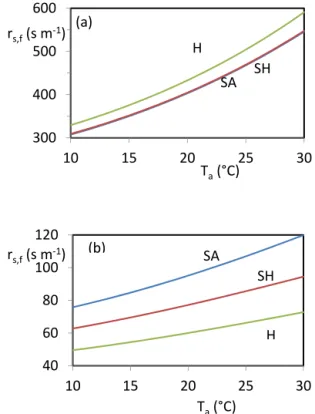
following FAO-56 (Table 16 and Fig. 32), where three types of climate are defined as a function of their relative humid-ity (Table 1). Figure 5 shows, for these three climatic envi-ronments, how the foliage surface resistance (rs, f), inferred
from the basal crop coefficient (Kcb), varies as a function of
air temperature. Two contrasting cases are considered with the assumptionf =1: one representing the initial stage of an annual crop withzh=0.5 m andKcb=0.5 (Fig. 5a) and the
other case, withzh=1.5 m andKcb=1.0, representing the
mid-season stage (Fig. 5b). These figures clearly show that crop coefficients cannot be easily translated into surface re-sistances because of the interference of climate characteris-tics such as air temperature and humidity (as shown here), but also wind speed and solar radiation (not shown) and other factors such as the soil evaporation coefficient (Ke).
Table 2 exemplifies for a typical crop and different climatic conditions the relative error made on the value ofrs, f when
the simplified formulation (Eq. 25) is used instead of the comprehensive one (Eq. 23). The relative error is generally lower than 10 % and much less under sub-humid conditions (around 1 %), which justifies the use of the simplified for-mula as an accurate approximation.
300 400 500 600
10 15 20 25 30
H
SH SA
Ta(°C) rs,f(s m-1) (a)
40 60 80 100 120
10 15 20 25 30
SA
SH
H (b)
Ta(°C) rs,f(s m-1)
Figure 5. Variation of foliage surface resistance (rs, f) inferred from the basal crop coefficient (Kcb)as a function of air temper-ature (Ta)for the three climatic environments (SA: semi-arid; SH: sub-humid; H: humid) described in Table 1 withua=2 m s−1, Ra=35 MJ m−2d−1 and Ke=0.1:(a)initial stage, zh=0.5 m, Kcb=0.5;(b)mid-season stage,zh=1.5 m,Kcb=1.
5 Conclusion and perspectives
We have shown that the FAO-56 dual crop coefficient ap-proach, where the crop coefficientKc is split into two
sep-arate coefficients (one for crop transpiration and another for soil evaporation), can be easily translated into a one-step approach based upon a Penman–Monteith type equation (Eq. 10), its surface resistance being the parallel sum of a soil and foliage resistance. This new form of the Penman– Monteith equation estimates fairly accurately crop evapo-transpiration when compared to a full two-layer model. It is also much less sensitive to an error on the crop parame-ter (represented by the surface resistance) than the FAO-56 methodology based on the crop coefficient. We have also shown that the foliage resistance of the one-step approach can be inferred from the crop coefficients (KcbandKe)in a
way similar to the Matt–Shuttleworth method. The interfer-ence of environmental factors, however, makes the calcula-tion somewhat hazardous.
two-step approach. In the one-step approach, four parame-ters should be adjusted to a specific crop: its albedo to es-timate the net radiation, its aerodynamic resistance and the two components of the surface resistance (soil and vegeta-tion). Albedo varies as a function of green canopy cover (or LAI). The aerodynamic resistance is calculated as a function of crop height (Eq. 14), provided the roughness length is cor-rectly determined (Eq. 16). The soil component of the surface resistance requires a specific parameterization as a function of top soil layer water content. Some empirical parameteri-zations already exist and should be thoroughly examined and tested. With regard to foliage resistance, although it can be inferred in principle from the basal crop coefficient, it is cer-tainly more recommendable to undertake experimental and bibliographical works in order to determine appropriate val-ues under standard conditions (i.e. non-stressed and well-managed crop). Given that foliage resistance is expressed as the simple ratio of leaf stomatal resistance to leaf area (see Eq. 12) and that LAI is an adjustable and experimen-tally accessible parameter, one can imagine that the mean leaf stomatal resistance could play the same role in the one-step approach as (and replace) the basal crop coefficient of the two-step approach. Tabulated values for different crops could be supplied and organized by group type in the same way as the crop coefficients in FAO-56. Only one value per crop could be needed, instead of the three values generally provided for crop coefficients, given that LAI values should be able to account for the necessary adjustment to crop cy-cle characteristics. It is worthwhile stressing, nevertheless, that the leaf stomatal resistance of a given crop under stan-dard conditions (which represents a minimum value) is sub-ject to the influence of other climatic environment parame-ters than water stress (i.e. temperature, humidity, radiation, CO2; Jarvis, 1976): its value should be specific to a
Appendix A: Calculation of the coefficient for soil evaporation (Ke)
According to FAO-56, the daily calculation ofKeis the result
of a relatively complex procedure based on Eq. (A1): Ke=minKr Kc, max−Kcb, fewKc, max, (A1)
whereKcbis the basal crop coefficient,Kc, maxis the
maxi-mum value ofKc=Kcb+Kefollowing rain or irrigation, and Kr is a dimensionless coefficient for the reduction of
evap-oration due to the depletion of water from the top soil. Its practical calculation relies on a daily water balance compu-tation for the surface soil layer detailed in FAO-56.fewis the
fraction of soil surface from which most evaporation occurs. Its calculation is also detailed in FAO-56.Kc, maxis obtained
from the following empirical equation: Kc, max
=max
1.2+
0.04(u2−2)−0.004(RHmin−45) zh
3 0.3
,
{Kcb+0.05}], (A2)
whereu2is the mean wind speed at 2 m height over grass and
Table A1.List of symbols.
Da Vapour pressure deficit at reference height (Pa) Db Vapour pressure deficit at blending height (Pa) Dm Vapour pressure deficit at canopy source height (Pa) d Canopy displacement height (m)
ET0 Reference crop evapotranspiration (mm d−1)
ETc Crop evapotranspiration under standard conditions (mm d−1) ea Vapour pressure at reference height (Pa)
em Vapour pressure at canopy source height (Pa) e∗(T ) Saturated vapour pressure at temperatureT (Pa) f= Rn/Rn,0(dimensionless)
G Soil heat flux of a given crop (W m−2) G0 Soil heat flux of the reference crop (W m−2) Kc Crop coefficient (dimensionless)
Kcb Basal crop coefficient (dimensionless)
Ke Coefficient for soil evaporation (dimensionless) LAI Leaf area index (m2m−2)
Ra Extraterrestrial solar radiation (MJ m−2d−1) Rn Net radiation of a given crop (W m−2) Rn,0 Net radiation of the reference crop (W m−2) Rn,f Net radiation of the foliage (W m−2) Rn,s Net radiation of the soil surface (W m−2)
ra Aerodynamic resistance between canopy source height and reference height (s m−1) ra,0 Aerodynamic resistance of the reference crop (s m−1)
rs,0 Surface resistance of the reference crop (s m−1)
ra, h Bulk air resistance of the canopy defined by Eq. (8) (s m−1) ra, v Defined by Eq. (8) and equal tora, hifra, f, v=ra, f,h(s m−1) rs, v Bulk surface resistance of the canopy defined by Eq. (9) (s m−1) ra,f,h Bulk boundary-layer resistance of the foliage for sensible heat (s m−1) ra, f,v Bulk boundary-layer resistance of the foliage for water vapour (s m−1) ra, f= ra,f,h=ra,f,v
ra, s Aerodynamic resistance between the soil surface and the source height (s m−1) rs, f Bulk stomatal resistance of the foliage (s m−1)
rs, l Mean stomatal resistance of the leaves per unit area of leaf (s m−1) rs, s Soil surface resistance to evaporation (s m−1)
Ta Air temperature at reference height (◦C) Tm Air temperature at canopy source height (◦C) Tf Foliage temperature (◦C)
Ts Soil surface temperature (◦C)
ua Wind speed at reference height (2 m; m s−1) ub Wind speed at blending height (50 m; m s−1) zr Reference height (m)
zh Mean canopy height (m)
zm Mean canopy source height (i.e.d+z0,m; m) z0,m Canopy roughness length for momentum (m) z0,h Canopy roughness length for scalar (m)
cp Specific heat of air at constant pressure (J kg−1◦C−1) ρ Air density (kg m−3)
γ Psychrometric constant (Pa◦C−1)
Appendix B: Parameterization of air resistances within the canopy
The parameterization commonly used to simulate the com-ponent air resistances taken and adapted from Shuttleworth and Wallace (1985), Choudhury and Monteith (1988), Shut-tleworth and Gurney (1990), Lhomme et al. (2012). The aerodynamic resistance between the substrate (with a rough-ness length z0, s of 0.01 m) and the canopy source height
(d+z0, m)is calculated as the integral of the reciprocal of
eddy diffusivity over the height range [z0, s,d+z0, m]: ra, s=
zhexp(αw) αwK(zh)
exp−αwz0,s/zh
−exp−αw(d+z0,m)/zh , (B1)
wherezhis the canopy height,αw=2.5 (dimensionless) and K(zh)is the value of eddy diffusivity at canopy height. With
the assumption that leaf area is uniformly distributed with height, the leaf boundary-layer resistance (two sides) per unit area of leaf is expressed as a function of wind speed at canopy heightu(zh)as
ra,l= αw
w/u(zh)
1/2
4α01−exp −α2w
, (B2)
wis leaf width (0.03 m) andα0is a constant equal to 0.005
(in m s−1/2). The eddy diffusivity at canopy height is
ex-pressed as K(zh)=k2ua(zh-d)/ln[(zr−d)/z0] and the
cor-responding wind speed u(zh)is obtained from an equation
Appendix C: Formulations of the two-layer model Following the reformulated expression of the two-layer model proposed by Lhomme et al. (2012), crop evaporation is given by
λE=
1+1 γ
(Pf+Ps) λEp
+
1 γ
PfRn,fra, f+Ps(Rn,s−G)ra, s
ra
, (C1)
whereλEprepresents the potential evaporation expressed as
λEp=
1(Rn−G)+ρcpraDa
1+γ . (C2)
The resistive terms are defined as follows: Pf=
raRs RfRs+RaRf+RaRs
,
Ps=
raRf RfRs+RaRf+RaRs
, (C3)
with Ra=
1+1
γ
ra, Rf=rs,f+
1+1
γ
ra, f,
Rs=rs,s+
1+1
γ
ra, s. (C4)
Net radiationRnis partitioned between the foliage and the
soil surface as a function of the LAI following Beer’s law:
Rn,s=Rnexp(−αLAI) , (C5)
Rn, f=Rn1−exp(−αLAI). (C6)
Edited by: N. Romano
References
Allen, R. G.: Using the FAO-56 dual crop coefficient method over an irrigated region as part of an evapotranspiration intercompar-ison study, J. Hydrol., 229, 27–41, 2000.
Allen, R. G., Pereira, L. S., Raes, D., and Smith, M.: Crop evapo-transpiration, Irrig. Drainage Paper No 56, United Nations FAO, Rome, 300 pp., 1998.
Choudhury, B. J. and Monteith, J. L.: A four-layer model for the heat budget of homogeneous land surfaces, Q. J. Roy. Meteor. Soc., 114, 373–398, 1988.
Doorenbos, J. and Pruitt, W. O.: Guidelines for predicting crop water requirements, FAO Irrigation and Drainage Paper no. 24. FAO, Rome, 144 pp., 1977.
Duchemin, B., Hadria, R., Erraki, S., Boulet, G., Maisongrande, P., Chehbouni, A., Escadafal, R., Ezzahar, J., Hoedjes, J. C. B., Kharrou, M. H., Khabba, S., Mougenot, B., Olioso, A., Ro-driguez, J. C., and Simonneaux, V.: Monitoring wheat phenology and irrigation in Central Morocco: on the use of relationships be-tween evapotranspiration, crop coefficients, leaf area index and remotely-sensed vegetation indices, Agric. Water. Manage., 79, 1–27, 2006.
Jarvis, P. G.: The interpretation of leaf water potential and stomatal conductance found in canopies in the field, Phil. Trans. R. Soc. London, Ser. B, 273, 593–610, 1976.
Katerji, N. and Rana, G.: FAO-56 methodology for determining wa-ter requirements of irrigated crops: critical examination of the concepts, alternative proposals and validation in Mediterranean region, Theor. Appl. Climatol., 116, 515–536, 2014.
Lhomme, J. P., Montes, C., Jacob, F., and Prévot, L.: Evaporation from heterogeneous and sparse canopies: on the formulations related to multi-source representations, Bound.-Lay. Meteorol., 144, 243–262, 2012.
Lhomme, J. P., Boudhina, N., and Masmoudi, M. M.: Techni-cal Note: On the Matt-Shuttleworth approach to estimate crop water requirements, Hydrol. Earth Syst. Sci., 18, 4341–4348, doi:10.5194/hess-18-4341-2014, 2014.
Mahfouf, J. F. and Noilhan, J.: Comparative study of various formu-lations of evaporation from bare soil using in-situ data, J. Appl. Meteorol., 30, 1354–1365, 1991.
Monteith, J. L.: Gas exchange in plant communities, in: Environ-mental Control of Plant Growth, edited by: Evans, L. T., Aca-demic Press, New York, 95–112, 1963.
Monteith, J. L.: Evaporation and the environment, Symp. Soc. Ex-perimental Biology, 19, 205–234, 1965.
Rosa, R. D., Paredes, P., Rodrigues, G. C., Alves, I., Fernando, R. M., Pereira, L. S., and Allen, R. G.: Implementing the dual crop coefficient approach in interactive software, 1. Background and computational strategy, Agric. Water Manage., 103, 8–24, 2012. Sellers, P. J., Heiser, M. D., and Hall, F. G.: Relations between sur-face conductance and spectral vegetation indices at intermediate (100 m2to 15 km2) length scales, J. Geophys. Res., 97, 19033– 19059, 1992.
Shuttleworth, W. J.: Towards one-step estimation of crop water re-quirements, T. ASABE, 49, 925–935, 2006.
Shuttleworth, W. J. and Wallace, J. S.: Calculating the water require-ments of irrigated crops in Australia using the Matt-Shuttleworth approach, T. ASABE, 52, 1895–1906, 2009.
Shuttleworth, W. J.: Putting the “vap” into evaporation, Hydrol. Earth Syst. Sci., 11, 210–244, doi:10.5194/hess-11-210-2007, 2007.
Shuttleworth, W. J.: Comment on “Technical Note: On the Matt-Shuttleworth approach to estimate crop water requirements” by Lhomme et al. (2014), Hydrol. Earth Syst. Sci., 18, 4403–4406, doi:10.5194/hess-18-4403-2014, 2014.
Shuttleworth, W. J. and Gurney, R. J.: The theoretical relation-ship between foliage temperature and canopy resistance in sparse crops, Q. J. Roy. Meteorol. Soc., 116, 497–519, 1990.
Shuttleworth, W. J. and Wallace, J. S.: Evaporation from sparse crops-an energy combination theory, Q. J. Roy. Meteorol. Soc., 111, 839–855, 1985.