Abstract— Maximum power point tracking (MPPT) allows the photovoltaic module to operate at its maximum power point. It is done using a converter that regulates the power that is drawn from the converter. By varying the duty cycle of the switches, the energy transferred through the converter can be precisely controlled. This paper deals with simulation of estimator for a digital tracking system used for simulation of maximum power point PV tracker using KALMAN Filter. For the simulation Back-Propagation and Radial Basis Network are used as Artificial Neural Network (ANN) tool. The objective of this paper is to discuss the use of KALMAN filter as an estimator in the area of photovoltaic cell power tracking.
Index Terms—RBF, BPNN, KALMAN Filter, Maximum power point tracker, PV cell.
I. INTRODUCTION
A solar cell is a semiconductor device that absorbs sunlight and converts it into electrical energy. Today's most common cell is a mass manufactured single p-n junction Silicon (Si) cell with efficiency up to about 17% [1]. Since 1973, the word “energy” has been continuously in the news. There has been shortage of oil in many parts of the world and the price of this commodity has increased steeply. It is by now clear that the fossil fuel era of non-renewable resources is gradually coming to an end. Oil and natural gas will be depleted first, followed eventually by coal.
In India the energy problem is very serious. In spite of discoveries of oil and gas off the west coast, the import of crude oil continues to increase and the price paid for it now dominates all other expenditure.
__________________________
Manuscripts received on 7th December, 2010 accepted on 22nd December 2010.
A. K. Goswami is Assistant Professor in the Department of Electrical Engineering, NIT Silchar, Assam-788010 ([email protected]) 91-9435740739.
H.R. Kamath is director Malwa Institute of Technology, Indore-452016 ([email protected]) 91-80109010964
The year 2008 (till April) the country has spent more than 61.62 billion dollars for the import of oil. This amount forms a major part of India’s import bill. The need for developing energy alternatives is thus evident and considerable research and development work is already in progress in this direction.
One of the promising options is to make more extensive use of renewable sources of energy derived from the sun. Solar energy can be used both directly and indirectly. It can be used directly in a variety of thermal applications like heating water or air, drying, distillation and cooking. A second way in which solar energy can be used indirectly is through the photovoltaic effect in which it is converted to electrical energy [2].
Use of photovoltaic (PV) technology to generate electricity is increasing world-wide. Over the past two decades PV has become well established in remote area power supply, where it can be the most cost-effective choice. PV is also becoming more common in grid connected applications, motivated by concerns about the contribution of fossil fuel use to the enhanced greenhouse effect and other environmental issues.
In designing any power generation system that incorporates photovoltaic (PV) there is a basic requirement to accurately estimate the output from the proposed PV array under operating conditions. Good system design is essential to provide reliable systems. An appropriately sized PV array enables consumers, especially of remote area systems, to receive a reliable energy supply at a reasonable cost [3].
It is well known that different PV technologies have different seasonal patterns of behavior. These differences are due to the variation in spectral response, the different temperature coefficients (TCs) of voltage and current and, in the case of amorphous silicon (a-Si) modules, the extra effect of photo – degradation and thermal annealing. However, PV modules are rated at standard test conditions (STC) of 1000W/m2, AM 1.5 and a module temperature of 25o C, and these conditions do not represent what is typically experienced under outdoor operation. Good system design assists in promoting the renewable energy industry. The increased use of PV, in turn, assists in attaining environmental goals [3].
II. REAL TIME DATA COLLECTION
The performance of a photovoltaic (PV) panel is affected by its orientation and its tilt angle with the horizontal plane. This is because both of these parameters change the amount of solar energy received by the surface of the PV panel. A mathematical model was used to estimate the total solar
RBF and BPNN Combi Model Based
KALMAN Filter Application for Maximum
Power Point Tracker of PV Cell
radiation on the tilted PV surface [4]. The tilt angle is also site dependent. The optimum slopes of PV panels at any latitude, for any surface azimuth angels and on a day or in a month of a year, have to be determined for design purposes. Definite value is rarely given by researchers for optimum tilt angles. Lunde [5] suggested Sopt = Ф ± 15º, Duffie and Beckman [6]
Sopt = (Ф + 15º) ±15º and Lewis [7] reported Sopt = Ф ± 8º. Also, researchers have reported that changing the tilt angle to its daily and monthly optimum values throughout the year does not seem to be practical, another possibility, such as changing the tilt angle once in a season [8].
In this study, two types of PV panels were used i.e. Poly-crystalline Silicon of 40 Watts (TATA BP Solar) and Amorphous Silicon of 43 Watts, Solarex (BP SOLAR) for data collection. The site selected was the roof top of the library building of Manipal Institute of Technology, Manipal University, Manipal, INDIA. Manipal is situated in the southern coastal belt (Latitude: 13° 20' 60 N, Longitude: 74° 46' 60 E) with average sunshine hours of 8 hours/day during almost 10 months in a year. For the creation of the PV Source modeling and training of the ANN model the basic requirement is the collection of a highly distributed range of I-V values. For the training of the proposed neural network, data collected in different seasons of 2009 and 2010 at Manipal University Campus, Manipal, India were used. Two different sets of solar panels are used for data collection. One of the panel of each set was placed at tilt angle of 13.2 degree and other panel constantly moved to different angles starting from 0 degree to 35 degree in the interval of 5 degrees, both panels were placed facing south. The readings were recorded for load voltage, load current, temperature and illumination levels at different time intervals in a day and also at different seasons from which maximum power and corresponding voltage (Vmax) and current (Imax) were recorded and Iavg calculated. The sample data collected for summer seasons are tabulated in table 1
Table 1 summer season- sunny day at tilt angle of 28.2 degree Time Angle (Degree) Illumination (Lux) Temperature of panel (ºC) Vload (V) Iavg (A) Pmax (W) 10.00 a.m.
28.2 74000 46 15.6 1.6 24.96
11.00 a.m.
28.2 95000 53 15 2.05 30.75
12.00 a.m.
28.2 109100 62 14.1 2.35 33.135
01.00 p.m.
28.2 101000 57 13.8 2.32 32.016
02.00 p.m.
28.2 93600 54 14.7 2.0 29.4
03.00 p.m.
28.2 75700 47 15.2 1.7 25.84
03.30 p.m.
28.2 61700 43 15.2 1.45 22.04
III. MATHEMATICAL MODEL OF PV CELLS
Solar Cells consist of a P-N junction built in a thin wafer of semiconductor. In dark, the output characteristics i.e. I-V has an exponential characteristic similar to that of a diode. The characteristic of this diode therefore sets the open voltage characteristics of the cell. The solar cell can be modeled into
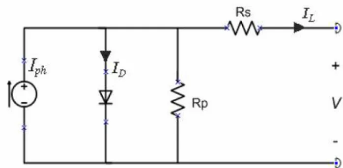
circuit equations by considering the effect of parallel resistance [9-13].The equivalent circuit model of a solar cell consists of a current generator and a diode plus series and parallel resistance as shown in figure 1.
Fig. 1 Simplified equivalent circuit of a solar cell considering Parallel Resistance
The photocurrent generated when the solar array is exposed to sunlight can be represented with a current source and the p-n junction transition area of the solar cell can be represented with a diode. The voltage and current relationship of the simplified solar cell is derived from Kirchhoff’s current law. Thus the mathematical equation for the output current of single cell is expressed as equation 1
0
s s
ph
sh
q( v
IR
v
IR
I
I
I
exp
I
AKT
R
⎡
⎛
+
⎞
⎤
+
=
−
⎢
⎜
⎟
−
⎥
−
⎝
⎠
⎣
⎦
(1)Where,
IL = I = load current,
Iph = Source Current.
Io = leakage or reverse saturation current, q = electron charge,
V = solar cell voltage, A= Ideality factor, k = Boltzmann constant, RS = series cell resistance,
RSh = shunt cell resistance.
The temperature of solar cell is expressed as
T = 3.12 +0.25 S+ 0.899Tm – 1.3WS +273 (2)
Where, Tm= ambient temperature, Ws=wind speed,
S = solar radiation.
Io can also be expressed in another form which depends on the temperature of the solar cell and is given as
3 0
1
1
or r rT
EG
I
I
(
)
exp((
) ( q
))
T
T
T
k
A
=
×
×
−
× ×
×
(3)Where, Ior= I at reference temperature at Tr for 301.18 ° K EG = band gap energy, Tr = reference temperature, T= cell temperature.
IPhis a function of incident solar radiation and cell
temperature and is given as
100
ph scr r
I
=
( I
+
ki( T
−
T )) S /
×
(4) Here, Iscr= short circuit current at Tr( )
exp
V
Rs V ns
I I npIph npIo Ko IRs I
Rsh Rsh ns ⎡ ⎧ ⎫ ⎤ ⎡ + ⎤= − ⎛ + ⎞ − − ⎢ ⎨ ⎜ ⎟⎬ ⎥ ⎢ ⎥ ⎣ ⎦ ⎢⎣ ⎩ ⎝ ⎠⎭ ⎥⎦ (5)
where np= number of parallel cells Ko=(q/(A*k*T)
3.1.1 Modeling of PV cells
The circuit equation obtained equation 1-5 for the P-V cell from the source model were coded using MATLAB and the output for it is as shown in figure 2.
Fig. 2. I-V characteristics of cell.
From the above figure it can be seen that as the voltage goes on increasing current starts decreasing with little variation in the initial stage. Here constant current curve shows current source characteristics of PV cell; where as varying I-V characteristic shows voltage source characteristics. Also the Power vs. Voltage curve is simulated and is shown in figure 3.
Fig. 3. I-V characteristics of cell.
Here it can be seen that as the voltage goes on increasing, power curve also increases with positive slope and after reaching the maximum power point it starts decreasing with negative slope with increase in voltage.
IV. MODELING OF KALMAN FILTER
Theoretically the KALMAN Filter is an estimator for what is called the linear-quadratic problem, which is the problem of estimating the instantaneous “ State” of a linear dynamic system perturbed by white noise-by using measurements linearly related to the state but corrupted by white noise. The
resulting estimator is statistically optimal with respect to any quadratic function of estimation error [14].
If we consider a system and wrote a system equation in matrix form
11 12 13 1 1 1
21 22 23 2 2 2
31 32 33 3 3 3
1 2 3 ln 1
.
.
.
.
.
.
.
.
.
.
.
.
.
.
.
.
.
.
.
.
.
.
.
.
n n nl l l n m
h
h
h
h
x
z
h
h
h
h
x
z
h
h
h
h
x
z
h
h
h
h
x
z
⎡
⎤ ⎡ ⎤ ⎡ ⎤
⎢
⎥ ⎢ ⎥ ⎢ ⎥
⎢
⎥ ⎢ ⎥ ⎢ ⎥
⎢
⎥ ⎢ ⎥ ⎢ ⎥
=
⎢
⎥ ⎢ ⎥ ⎢ ⎥
⎢
⎥ ⎢ ⎥ ⎢ ⎥
⎢
⎥ ⎢ ⎥ ⎢ ⎥
⎢
⎥ ⎢ ⎥ ⎢ ⎥
⎢
⎥ ⎢ ⎥ ⎢ ⎥
⎣
⎦ ⎣ ⎦ ⎣ ⎦
(6 )Or
[ ][ ] [ ]
H
X
=
Z
(7 ) Then consider the problem of solving for that value of an estimatex
that minimizes the “estimated measurement error”Hx
−
z
.It is characterize that estimation error in terms of its Euclidean vector norm
Hx
−
z
, or, equivalently, its square:2 2
( )
e x
=
Hx
−
z
(8 )=
2
1 1
m n
ij j i
i j
h x
z
= =
⎡
⎤
−
⎢
⎥
⎣
⎦
∑ ∑
(9 ) This is a continuously differentiable function of the n unknownsx x x
1,
2,
3...,
x
n. This is functione x
2( )
→ ∞
. Consequently, it will achieve its minimum value where all its derivatives with respect to thex
k are zero. There as n such equations of the form2
0
k
de
dx
=
(10 )=
1 1
2
m n
ik ij j i
i j
h
h x
z
= =
⎡
⎤
−
⎢
⎥
⎣
⎦
∑ ∑
(11) For k=1, 2, 3……n, note that in the last equation the expression{
}
1
n
ij j i i
j
h x
z
Hx
z
=
− =
−
∑
(12 ) The ith row ofHx
−
z
, and the outermost summation is equivalent to the dot product of the kth column of H withHx
−
z
. Therefore equation 11 can be written as[
]
HT=
11 21 31 1
12 22 32 2
13 23 33 3
1 2 3
. .
. .
. .
.
.
.
. .
.
.
.
.
. .
.
. .
mm
m
n n n mn
h
h
h
h
h
h
h
h
h
h
h
h
h
h
h
h
⎡
⎤
⎢
⎥
⎢
⎥
⎢
⎥
⎢
⎥
⎢
⎥
⎢
⎥
⎢
⎥
⎢
⎥
⎣
⎦
(16)
The equation
H Hx
T=
H z
T (17) is called the normal equation or the normal form of the equation for the linear least squares problem. It has precisely as many equivalent scalar equations as unknowns. The GRAMIAN of the linear least square problem. The normal equation has the solution1
(
T)
Tx
=
H H
−H z
Provide that the product G=HTH is non singular
V. SIMULATION MODEL OF BACK PROPAGATION NEURAL NETWORK
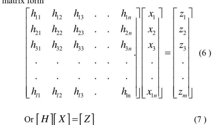
For the SIMULINK model of Artificial Neural Network, first the modeling of network is done using MATLAB coding [15-17]. Then the SIMULINK model is generated using MATLAB command ‘GENSIM’. SIMULINK model of Back-Propagation Neural Network architecture is shown in Fig. 3 where two layers of neurons are used i.e. input layer and output layer. For input and output layer the transfer function used is tansig whose value lies between -1 and 1.
Fig. 3: SIMULINK diagram of BP NN architecture
VI. SIMULATION MODEL OF RADIAL BASIS NEURAL NETWORK Radial Basis Function (RBF) network is modeled with two layers of neurons using MATLAB coding and SIMULINK model is generated using MATLAB command ‘GENSIM’ [15-17]. The transfer function used for the input layer is ‘RADBAS’ and for the output layer is ‘PURELIN’. The SIMULINK model diagram is shown in Figure 4.
Fig. 4: Simulink diagram of RBF NN architecture
VII. SIMULATION MODEL OF ANN KALMAN FILTER As per proposed model of KALMAN Filter first the comparison of BP/RBF output is done with the error of BP/RBF output and mathematical model output for the same input condition i.e. load voltage, illumination level and temperature[18-19]. The general diagram for both the BP and RBF along with KALMAN filter is shown in Figure. 5.
Fig.5: SIMULINK diagram of BP/RBF neural network and mathematical model
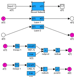
Since the input required for KALMAN filter is discrete so the output of BP model and mathematical model is passed through zero order hold to make the signal discrete. Results obtained from simulation of mathematical model and back-propagation filter and radial basis and back-propagation filter are shown in Figure 6 and 7 respectively [20].
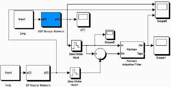
VIII. SIMULATION OF DUAL STRUCTURE ANN KALMAN FILTER MODEL
Fig.6: Result of BP and mathematical models
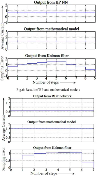
Fig. 7: Result of RBF and mathematical models
Fig. 8: Result of RBF and BP COMBI model
IX. RESULT AND DISCUSSION
The implementation of KALMAN estimator helps in estimating the error convergence duration of different models to estimate the model tracking accuracy. It is estimated that BPNN vs mathematical model error converges to zero in 9 samples Fig. 6, RBF vs mathematical model error converges to zero in seven samples Fig. 7 and RBF vs BPNN error converges to zero in 182 samples Fig. 8. Since RBF model gives an error convergence in minimum sampling rate so it will be the most suitable model for estimating tracking error if Model Reference Adaptive Controller (MRAC) scheme is used for solar tracker.
X. CONCLUSIONS
This paper has evolved a maximum power point tracker using digital detection and estimation technique. Since the data were collected off line to test and analyze the behavior of an intelligent tracker based on ANN detector and KALMAN Estimator. KALMAN filter is based on recursive technique in which, a one step ahead predictor is used on the current state and white noise estimates generated by the standard model and detector model. This combination results into the simulation of reduced error tracker. In the present case the estimator detector combination for BPK and mathematical model, RBF and mathematical model and BPK and RBF models have been tested for maximum current tracking. It has been found that RBF and Mathematical model error convergence takes minimum sample steps. Thus it can be concluded that RBF type model using KALMAN Filter is ideal for maximum power point tracking when maximum current has to be tracked in the actual Model Reference Adaptive Control of Solar Tracking System for maximum current.
ACKNOWLEDGMENT
The authors would like to acknowledge the help provided by Manipal Institute of Technology, Manipal University, Manipal, INDIA for providing the technical data for this work. The authors sincerely thank the Department of Electrical Engineering, NIT Silchar for providing the facility for completing this work.
REFERENCES
[1]K.H. Hussein, I. Muta, T. Hoshino, M. Osakad, “Maximum photovoltaic power tracking: an algorithm for rapidly changing atmospheric condition”, IEE Proceedings – Generation, Transmission and Distribution -January 1995, Vol. 142, no. 1, pp. 59-64.
[2]Yeong-Chau Kuo, Tsorng-Juu Liang, Jiann-Fuh Chen: “Novel maximum-power-point-tracking controller for photovoltaic energy conversion system”
Industrial Electronics, IEEE Transactions on Volume 48, Issue 3, June
2001 Pages: 594 – 60.
[3]Hussein K.H., Muta I., Hoshino T., Osakada, M.: “Maximum photovoltaic power tracking: an algorithm for rapidly changing atmospheric conditions”.
Generation,Transmission and Distribution, IEE Proceedings-Volume 142
Issue 1, Jan. 1995,Pages: 59 – 64.
Fig. 9: SIMULINK diagram of RBF and BP NN COMBI model
[5]Murat Kacira, Mehmet Simsek, Yunus Babur, Sedat Demirkol,
“Determining optimum tilt angles and orientations of photovoltaic panels”,
Elsevier Journal of Renewable Energy, Vol-29 (2004),pp: 1265–1275. [6] Lunde PJ “Solar thermal engineering”, New York, John Wiley and Sons,
Inc., 1980, 635 p
[7] Duffie JA, Beckman WA. “Solar engineering of thermal processes”. New York:Wiley; 1982.
[8] Lewis G. “Optimum tilt of solar collector”, Solar and Wind Energy 1987, Vol-4, pp :407–10.
[9] Yakup MAM, Malik AQ., “Optimum tilt angle and orientation for solar
collector in Brunei Darussalam”, Elsevier Journal Renewable Energy
2001, Vol-24, pp 223–34
[10] Durisch, W.; Mayor, J.-C. “Application of a generalized current/voltage model fosolar cells to outdoor measurements on a SIEMEN
SM 110-modulePhotovoltaic Energy Conversion, Volume 2, Issue , 12-16
May 2003,pp: 1956 -1959 .
[11] J. A. Gow, C. D. Manning “Development of a photovoltaic array model for use in power electronics simulation studies,” IEE Proceedings on
Electric Power Applications, , March 1999,vol. 146, no. 2, pp. 193-200.
[12] M. Buresch “Photovoltaic Energy Systems Design and Installation”, New York McGraw-Hill Book Co, 1983, 347 p
[13] Green, “Efficiency enhancements in crystalline silicon solar cells by alloying with germanium” Elsevier journal of Solar energy materials and solar cells, ISSN 0927-0248 1992, vol. 28, pp. 273-284.
[14] Mohinder S. Grewal and Angus P. Andrews, “Kalman filtering theory and practice using Matlab”, Second edition, 2001 Jhon Wiley & Sons, Inc.
[15] M. Veerachary, T. Senjyu, and K. Uezato, “Neural-network-based maximum-power- point tracking of coupled-inductor interleaved-boost converter-supplied PV system using fuzzy controller,” IEEE Trans. Ind. Electron. , Aug. 2003, vol. 50, pp. 749-758.
[16] A. Hussein, K. Hirasawa, J. Hu, and J. Murata, “The dynamic performance of photovoltaic supplied dc motor fed from DC-DC converter and controlled by neural networks,” in Proc. 2002 International Joint Conf. on Neural Networks, 2002, pp. 607-612.
[17] L. Zhang, Y. Bai, and A. Al-Amoudi, “GA-RBF neural network based maximum power point tracking for grid-connected photovoltaic systems,” in International Conf. on Power Electron., Machines and Drives, 2002, pp. 18-23.
[18] Julier, Simon and Jeffrey Uhlman. “A General Method of Approximating Nonlinear Transformations of Probability Distributions”, Robotics Research Group, Department of Engineering Science, University of Oxford, 1995.
[19] Rolf Iserman, “Digital Control Systems”, Second Revised Edition, Springer – Verlag Berlin, Heidelber.