UNIVERSIDADE FEDERAL DE MINAS GERAIS
ESCOLA DE ENGENHARIA
MASTER THESIS
Control Strategies of a Tilt-rotor UAV for Load
Transportation
Marcelino Mendes de Almeida Neto
Belo Horizonte
UNIVERSIDADE FEDERAL DE MINAS GERAIS
ESCOLA DE ENGENHARIA
MASTER THESIS
Control Strategies of a Tilt-rotor UAV for Load
Transportation
Thesis submitted to the Programa de P´os-Gradua¸c˜ao em Engenharia El´etrica, Escola de Engenharia,
in partial fulfillment of the requirements for the degree of Master in Electrical Engineering
at the
Universidade Federal de Minas Gerais.
By
Marcelino Mendes de Almeida Neto
UNIVERSIDADE FEDERAL DE MINAS GERAIS
ESCOLA DE ENGENHARIA
MASTER THESIS
Control Strategies of a Tilt-rotor UAV for Load
Transportation
Acknowledgements
First of all, I would like to thank my parentsAmerico Almeida and Simone Teixeira,
who always supported me and were source of pride, admiration and reference for my personal e professional growth.
To my brothers Anna Laura Almeida, Americo Almeida and Pedro Arthur Almeida:
friends for an entire life.
To Ana Christine, for cheering up even more my day-to-day.
Special thanks to Prof. Guilherme Raffo for guiding and assisting me on this
ex-traordinary experience for the achievement of the Master Degree.
I thank Prof. Bruno Adorno, my informal co-advisor.
Thanks to Prof. Patr´ıcia Pena, who helped me with my first steps in the
univer-sity. She guided (and still guides) me both in personal and professional life. Not only a professor: a second mother.
I am very much thankful to Prof. Ronaldo Pena. He inspired me right at the beginning
of my undergraduate engineering course and paved the way for my past and future steps. To the members of the ProVant team, who were always on my side through this
journey. Special thanks to Werner Andrade, who helped me designing some figures for
my text.
To the members and cohabitants of LACSED:Luis Henrique,Ramon Dur˜aes,Gustavo
Vieira, Pedro Braga, Hugo Bravo, among other passers-by.
To thePrograma de P´os Gradua¸c˜ao em Engenharia El´etrica UFMG and all its faculty
for their teaching excellency. They are able to expand one’s conceptions about engineering,
life, the universe and everything rather than just providing42 as an answer.
(...) Nobody is gonna hit as hard as life. But it ain’t about how hard you hit: It’s about how hard you can get hit and keep moving forward. That’s how winning is done!
Abstract of the Thesis submitted to the Programa de P´os-Gradua¸c˜ao em Engenharia El´etrica, Escola de Engenharia, in partial fulfillment of the requirements for the degree of Master in
Electrical Engineering at the Universidade Federal de Minas Gerais.
Control Strategies of a Tilt-rotor UAV for Load Transportation
Marcelino Mendes de Almeida Neto
August / 2014
Advisors: Guilherme Vianna Raffo
Area of Concentration: Systems Engineering and Automation
Keywords: Unmanned Aerial Vehicles, Tilt-rotor, Load Transportation,
H∞ Control, Input-Output Feedback Linearization, Path
Tracking, Kalman Filter
This dissertation presents control strategies to solve the problem of suspended load trans-portation by a Tilt-rotor Unmanned Air Vehicle (UAV) passing through a desired tra-jectory. For the present study, it is important for the aircraft to maintain itself and the load stable even in the presence of external disturbances, parametric uncertainties and measurement errors.
In general, a precise dynamic model of a system is needed in order to design advanced control strategies to it. Therefore, a rigorous dynamic model is derived for the Tilt-rotor UAV with suspended load using Euler-Lagrange formulation. After obtaining the model, it is then possible to design control laws that satisfy the desired specifications. Con-sequently, linear and nonlinear control laws are designed.
In order to design linear control laws, the system is linearized around its operation point. Two linear control laws are designed: one using D-stability control design and the
second using simultaneous D-stability and minimization of the H∞ norm.
As for the nonlinear control design, a three-level cascade strategy is proposed. Each level of the cascade system executes a control law through the method of input-output feedback linearization. Each one of these levels controls a different group of the system’s state variables until the aircraft becomes fully stable. Two path tracking controllers are specified for this strategy. The first considers the load only as a disturbance and does not actuate to avoid its swinging. The second controller, on the other hand, seeks to find a compromise between path tracking and reducing the load’s swing. At last, as proof of concept, the nonlinear strategy is modified so that the aircraft is able to stabilize an inverted pendulum.
in Electrical Engineering na Universidade Federal de Minas Gerais.
Control Strategies of a Tilt-rotor UAV for Load Transportation
Marcelino Mendes de Almeida Neto
August / 2014
Orientador: Guilherme Vianna Raffo
´
Area de Concentra¸c˜ao: Engenharia El´etrica
Palavras-chave: Ve´ıculos A´ereos N˜ao Tripulados, Tilt-rotor, Transporte de
Carga, Controle H∞, Lineariza¸c˜ao por Realimenta¸c˜ao de
Sa´ıda, Seguimento de Trajet´orias, Filtro de Kalman
Nessa disserta¸c˜ao s˜ao apresentadas estrat´egias de controle para solucionar o problema de transporte de carga suspensa ao longo de uma trajet´oria desejada por um Ve´ıculo A´ereo N˜ao Tripulado (VANT) na configura¸c˜ao Tilt-rotor. Para o presente estudo, ´e importante que a aeronave seja capaz de manter tanto a si mesma quanto a carga transportada est´avel mesmo na presen¸ca de perturba¸c˜oes externas, incertezas param´etricas e erros de medi¸c˜ao.
Em geral, ´e importante que se tenha um modelo dinˆamico preciso do sistema para que se possa projetar estrat´egias de controle avan¸cadas para o mesmo. Dessa forma, um modelo dinˆamico para o VANT Tilt-rotor com carga suspensa ´e rigorosamente derivado usando a formula¸c˜ao de Euler-Lagrange. Com o modelo obtido, ´e poss´ıvel ent˜ao projetar leis de controle que satisfa¸cam as especifica¸c˜oes desejadas. Para tanto, leis de controle lineares e n˜ao lineares s˜ao projetadas.
Para projetar leis de controle lineares, lineariza-se o sistema em torno do seu ponto de opera¸c˜ao. Com o sistema linearizado, duas leis de controle s˜ao projetadas: uma por
D-estabilidade e outra que leva em considera¸c˜ao D-estabilidade e a normaH∞
simultanea-mente.
J´a para o projeto do sistema de controle n˜ao linear, uma estrat´egia em cascata ´e pro-posta. Cada n´ıvel do sistema em cascata executa uma lei de controle atrav´es do m´etodo de lineariza¸c˜ao por realimenta¸c˜ao de sa´ıda, sendo considerados trˆes n´ıveis. Cada um desses n´ıveis controla um grupo diferente de vari´aveis do sistema at´e que a aeronave esteja est´avel por completo. Para essa estrat´egia, dois controladores para seguimento de trajet´oria s˜ao especificados. O primeiro controlador considera a carga apenas como uma perturba¸c˜ao e n˜ao atua para impedi-la de balan¸car, preocupando-se apenas com o seguimento de tra-jet´oria. O segundo controlador, por sua vez, busca encontrar um compromisso entre seguir a trajet´oria e reduzir o balan¸co da carga. Por fim, como prova de conceito, a estrat´egia n˜ao linear ´e modificada de forma a fazer com que a aeronave estabilize um pˆendulo inver-tido.
Contents
Contents i
List of Figures iv
List of Tables vii
Acronyms ix
Notation x
1 Introduction 1
1.1 Motivation . . . 1
1.1.1 Historical Background . . . 2
1.2 State of the Art . . . 8
1.2.1 Tilt-rotor UAV control . . . 8
1.2.2 Load Transportation . . . 10
1.3 Justification and Objectives . . . 11
1.4 Structure of the Text . . . 13
1.5 List of Publications . . . 14
2 Modelling 15 2.1 Introduction . . . 15
2.2 Generalized Coordinates . . . 16
2.3 Kinematics . . . 18
2.4 Dynamics using Euler-Lagrange Formulation . . . 18
2.4.1 Inertia Matrix . . . 19
2.4.2 Coriolis and Centripetal Matrix . . . 23
2.4.3 Gravity Force Vector . . . 23
2.4.4 Input Force Vector . . . 24
2.4.5 Drag Force Vector . . . 26
2.5 State-Space Representation of the System . . . 26
2.6 System Design Parameters . . . 27
3 Linear Control Strategies 29
3.1 Introduction . . . 29
3.2 Linear Control Systems Theory . . . 30
3.2.1 Controllability of Linear Systems . . . 30
3.2.2 Stability of Linear Systems. . . 31
3.2.3 Linear Matrix Inequalities . . . 32
3.2.4 D-stability . . . 32
3.2.5 Linear H∞ Controllers . . . 35
3.3 Tilt-Rotor Linear Control . . . 37
3.3.1 Equilibrium Point and Linear Model . . . 38
3.3.2 Controllability of the Tilt-rotor UAV . . . 39
3.3.3 D-stable Controller Design . . . 39
3.3.4 D-Stable H∞ Controller Design . . . 40
3.4 Simulation and Results . . . 41
3.5 Conclusions . . . 43
4 Nonlinear Control Strategies 47 4.1 Introduction . . . 47
4.2 Nonlinear Control Theory . . . 48
4.2.1 Preliminary Theory on Nonlinear Systems . . . 49
4.2.2 Input-Output Feedback Linearization . . . 50
4.3 Tilt-rotor Nonlinear Control . . . 54
4.3.1 First-level Feedback Linearization . . . 54
4.3.2 Second-level Feedback Linearization . . . 58
4.3.3 Third-level Feedback Linearization . . . 61
4.3.3.1 Performance Improvement of the Load’s Swing . . . 68
4.3.4 Inverted Pendulum Control Strategy . . . 69
4.4 Simulation Results . . . 71
4.4.1 Comparison between NLPT and NLLS . . . 71
4.4.2 Comparison between NLLS and Linear H∞ . . . 72
4.4.3 Inverted Pendulum . . . 76
4.5 Conclusions . . . 78
5 State Estimation 89 5.1 Introduction . . . 89
iii
5.3 System Modelling for State Estimation . . . 90
5.4 Kalman Filter with Unknown Inputs . . . 94
5.5 Simulation Results and Analysis . . . 96
5.6 Conclusion . . . 98
6 Conclusions 105 6.1 Future Works . . . 107
Bibliography 109 A Theory on Robotics 113 A.1 Rotation Matrices. . . 113
A.2 Skew Symmetric Matrices . . . 115
List of Figures
1.1 Focke Achgelis FA-269 (Courtesy of Aviastar). . . 3
1.2 Transcendental 1-G (Courtesy of Aviastar). . . 3
1.3 McDonnell Aircraft Co. XV-1 compound helicopter (Courtesy of Aviastar). 4 1.4 Bell Helicopter Company XV-3 Tilt-rotor aircraft (Courtesy of Aviastar). . 4
1.5 Bell Helicopter XV-15 Tilt-rotor aircraft (Courtesy of Wikipedia). . . 5
1.6 Osprey V-22 Tilt-rotor (Courtesy of Wikipedia). . . 5
1.7 Augusta Westland AW609 Tilt-rotor (Courtesy of Wikipedia). . . 6
1.8 Cruise Speeds of Various Helicopters (Courtesy of FindTheBest). . . 6
1.9 Cruise Speeds of Various Airplanes (Courtesy of FindTheBest). . . 7
1.10 Bell Eagle Eye TR911X (Courtesy of BlueSkyRotor). . . 7
1.11 Lockheed-Martin’s ARES concept (Courtesy of Lockheed Martin). . . 8
1.12 ProVant Model 1.0. . . 8
1.13 ProVant Model 2.0. . . 9
1.14 ProVant Model 2.0 with Suspended Load. . . 12
2.1 Tilt-rotor UAV. . . 16
2.2 Tilt-rotor UAV frames and variables definition. . . 17
3.1 H∞ diagram block. . . 36
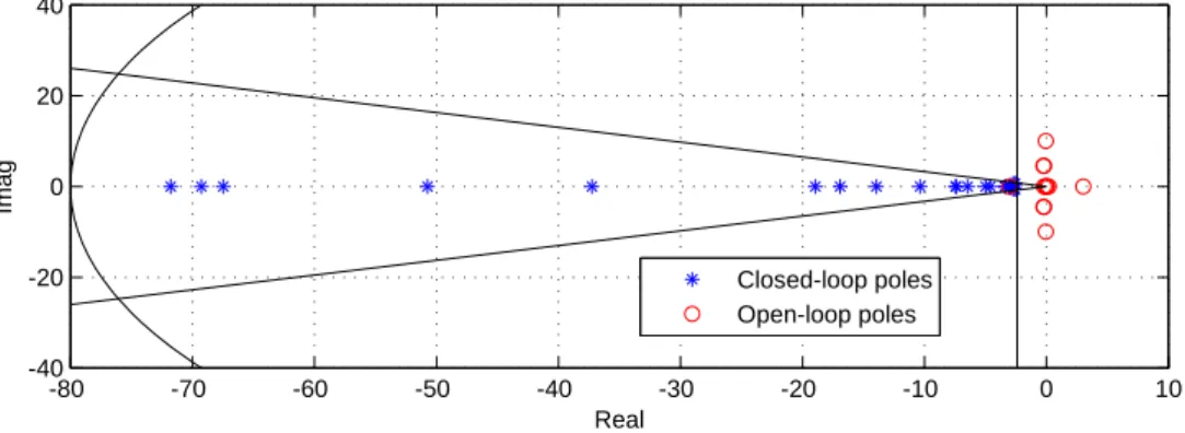
3.2 Allocation of poles via D-Stability. . . 40
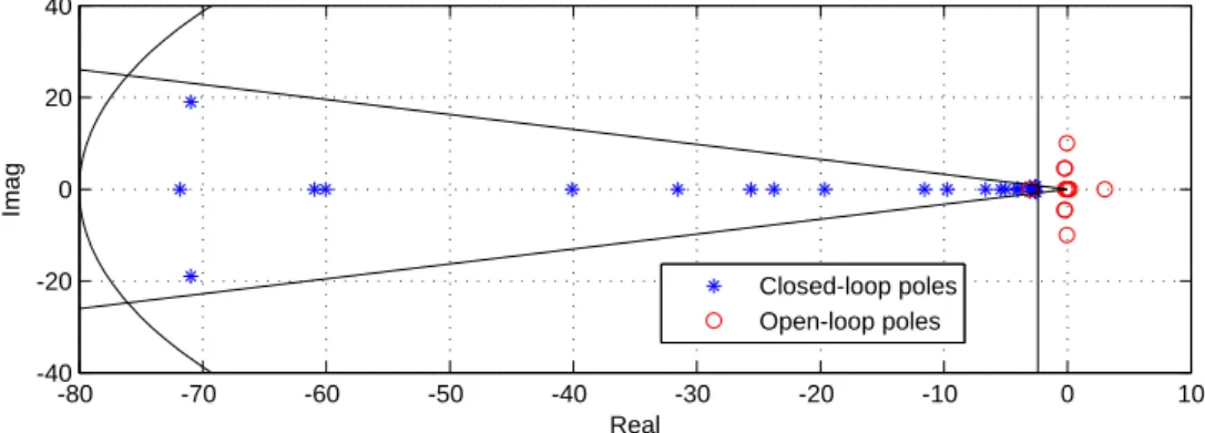
3.3 Allocation of poles via D-Stability with minimization of the H∞ norm. . . 41
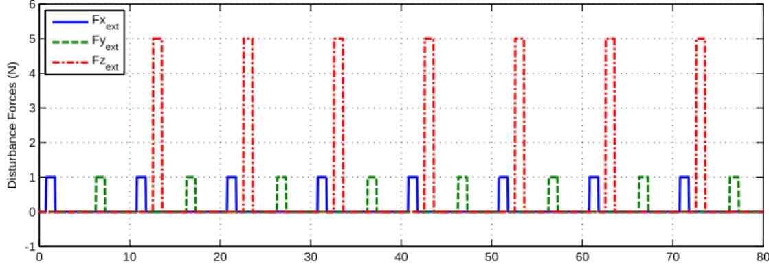
3.4 System disturbances in function of time. . . 42
3.5 Path tracking of the aircraft for both D-stable and H∞ controllers.. . . 43
3.6 Tracking errors for D-stable and H∞ controllers. . . 44
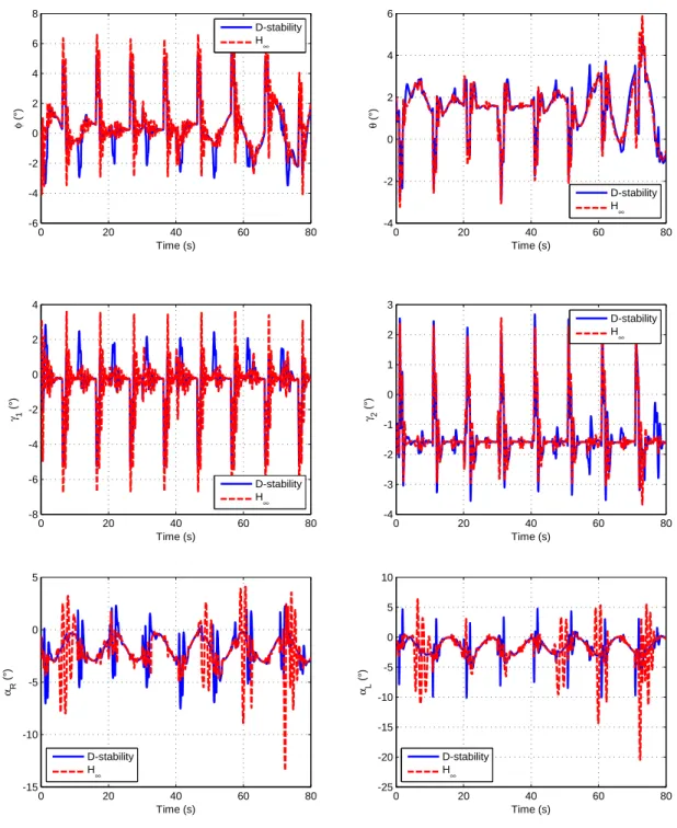
3.7 Body and Load angles for D-stable and H∞ controllers. . . 45
3.8 Inputs of the system for D-stable and H∞ controllers. . . 46
4.1 Nonlinear Feedback Linearization Cascade Control Strategy. . . 48
4.2 Inverted Pendulum Projections. . . 70
4.3 Path tracking of the aircraft for NLPT and NLLS. . . 72
4.4 Tracking error on NLPT and NLLS. . . 73
4.6 Inputs of the system using NLPT and NLLS.. . . 75
4.7 Path tracking of the aircraft for NLLS andH∞. . . 76
4.8 Tracking error on NLLS andH∞. . . 77
4.9 Body and Load angles on NLLS andH∞.. . . 78
4.10 Inputs of the system using NLLS and H∞. . . 79
4.11 Path tracking of the aircraft for NLLS and H∞ for a faster trajectory. . . . 80
4.12 Path tracking of the aircraft for NLLS and H∞ for harsher disturbances. . 81
4.13 Tracking error on NLLS and H∞ for Nonzero Initial Conditions. . . 82
4.14 Body and Load angles on NLLS and H∞ for Nonzero Initial Conditions. . 83
4.15 Path tracking of the aircraft with inverted pendulum. . . 84
4.16 Aircraft’s position and attitude for the inverted pendulum. . . 85
4.17 αand γ in function of time for the inverted pendulum. . . 86
4.18 Inputs for the inverted pendulum. . . 87
5.1 System disturbances for the LKFUI simulation. . . 98
5.2 Path tracking of the aircraft for the LKFUI simulation. . . 99
5.3 Position estimation error in function of time for the LKFUI simulation. . . 100
5.4 Tracking error for the LKFUI simulation. . . 101
5.5 Body and Load angles for the LKFUI simulation. . . 102
5.6 Inputs of the system for the LKFUI simulation. . . 103
List of Tables
2.1 System Parameters. . . 28
3.1 Mean-square-error comparison between D-stable and H∞ controller. . . 42
3.2 IAVU Index comparison between D-stable and H∞ controller. . . 42
4.1 Controllers parameters for the two first Feedback-Linearizations. . . 61
4.2 Controllers parameters for the whole cascade system. . . 68
4.3 Controllers parameters for load control. . . 69
4.4 Controllers parameters for the inverted pendulum. . . 71
4.5 Mean-square-error comparison between NLPT and NLLS. . . 72
4.6 IAVU Index comparison between NLPT and NLLS. . . 73
4.7 IAVU Index comparison between NLLS and H∞. . . 76
4.8 Mean-square-error comparison between NLLS and H∞. . . 77
4.9 IAVU Index for the Inverted Pendulum. . . 79
5.1 Translational controllers parameters for use with LKFUI. . . 98
Acronyms
VTOL Vertical Take-off and Landing
DH Denavit-Hartenberg Convention
UAV Unmanned Aerial Vehicle
DOF Degrees of Freedom
FKM Forward Kinematic Model
LMI Linear Matrix Inequalities
MIMO Multiple Input Multiple Output
FL Feedback Linearization
ISFL Input-State Feedback Linearization
IOFL Input-Output Feedback Linearization
PFL Partial Feedback Linearization
PD Proportional-Derivative
PID Proportional-Integral-Derivative
NLPT Nonlinear Controller for Path Tracking
NLLS Nonlinear Controller for Reduced Load Swing
GPS Global Positioning System
Notation
Notation
a Italic lower case letters denote scalars
a Boldface italic lower case letters denote vectors
A Boldface italic upper case letters denote matrices
Symbols
0n×m Zero matrix with n lines and m columns
In Identity matrix of dimension n
k Number of samples
x Vector of nth order, where x
i, i= 1. . . n, x∈ ℜn
xT Transpose vector of x
˙
x Time-derivative of x
ˆ
xk|j Prediction of the state vector xat instant k using measured
inform-ation
up to instant j
x0 Initial condition of x
xr Reference vector of the variable x
εq Tracking error for the generalized variable q
Model Notation
fR Right rotor’s thrust
fL Left rotor’s thrust
ταR Tilting torque for the right rotor
ταL Tilting torque for the left rotor
I Fixed inertial frame
B Moving body frame
C1 Frame rigidly attached to the main body’s center of mass
C2 Frame rigidly attached to the right rotor’s center of mass
C3 Frame rigidly attached to the left rotor’s center of mass
C4 Frame rigidly attached to the suspended load’s center of mass
φ Roll angle
θ Pitch angle
ψ Yaw angle
ξ= [xI yI zI]T Translation between the origins of frames I and B
η= [φ θ ψ]T The main body attitude with respect to frame I
αR, αL Tilt angles of the right and left rotors, respectively
γ1, γ2 Degrees of freedom of the suspended load
β Constant rotation of right and left rotors around xCi, for i= 1,2
dBi = [dB
xi dByi dBzi]T Translation between the origins of frames B and Ci, fori= 1,2,3,4
l Distance between frame B and the suspended load’s center of mass
RBA Rotation matrix from generic frame A to generic B
pAi point rigidly attached to frame Ci represented in generic frame A
M(q) Euler-Lagrange’s inertia matrix
C(q,q˙) Euler-Lagrange’s coriolis and centrifugal forces matrix
G(q) Euler-Lagrange’s gravitational force vector
F(q) Euler-Lagrange’s independent input force vector
Fext Euler-Lagrange’s external unknown force vector
Fdrag Drag force vector
µ Drag coefficients matrix
K Kinetic energy of the whole system
Ki Kinetic energy of theith body
vI
i Velocity of the center of mass of bodyi with respect to frameI
ωBAB Angular velocity of generic frame B with respect to a generic frame
A
represented in frameB
S(·) Skew symmetric matrix
ρi Mass density of body i
m Total mass of the helicopter with suspended load
mi Mass of theith body
Ii Inertia tensor of body i
Ji Inertia tensor of a rotated and displaced body
Wη Euler matrix expressed in the body-fixed frame
P Potential energy of the whole system
Pi Potential energy of theith body
g= [0 0 −gz]T Gravity vector
gz Gravity acceleration
b Thrust coefficient of the rotors
kτ Drag coefficient of the propellers
TI Translational Force Vector
τ Attitude Force Vector
Γ Control action vector
B(q) Force matrix (input coupling matrix)
Controllers Notation
d Exogenous disturbance vector
u Control effort vector
A Linear state matrix
Bu Linear input matrix
Bg Linear external input matrix
K Control matrix
V(x) Lyapunov function
γ Attenuation level of the H∞ problem
H(s) Transfer function between the input signal and the output signal z
kH(s)k∞ H∞-norm of the transfer function H(s)
Notation xiii
f(x) Nonlinear drift vector field
gu(x) Nonlinear steering vector field
gd(x) Nonlinear external steering vector field
h(x) Nonlinear output vector field
Df, Jacobian matrix associated to the vector field f(x)
ri Relative degree of the ith output
Φ(x) Diffeomorphism function
z Transformed state-space vector
v Transformed input vector
ϑ Internal dynamics state-space vector
qc Controllable variables vector
qu Uncontrollable variables vector
σ(p) Saturation function
State Estimation Notation
Ts GPS’s sampling time
τs Controller’s sampling time
wk Process noise
Q Process noise’s covariance matrix
vk Measurement noise
Rk Measurement noise’s covariance matrix
E[·] Expected value operation
Lk Kalman Filter’s gain matrix
ek|k−1 Forecast error
νk|k−1 Innovation
ek|k Data-assimilation error
Pkxx|k−1 Forecast error covariance
Pkyy|k−1 Innovation covariance
Pkxy|k−1 Cross covariance
Chapter 1
Introduction
Sum´
ario
1.1 Motivation . . . 1
1.1.1 Historical Background . . . 2
1.2 State of the Art . . . 8
1.2.1 Tilt-rotor UAV control. . . 8
1.2.2 Load Transportation . . . 10
1.3 Justification and Objectives . . . 11
1.4 Structure of the Text . . . 13
1.5 List of Publications . . . 14
1.1
Motivation
It is a moment of great development on Unmanned Aerial Vehicles (UAV) research. Many fields of control and robotics, such as sensor fusion, computer vision, rapid prototyping, state estimation and control methodologies improved the performance of this kind of sys-tems. This allowed UAV’s to be produced with low cost, becoming accessible to numerous research facilities and hobbyists all around the world.
As for the applications, there is a vast list of UAV uses: cargo delivery, surveillance, field recognition, cave exploration, cinematographic filming, military purposes, water and spray over plantations, 3-D mapping, search and rescue, wildlife research, among many others. In short, UAVs are being increasingly used for diverse civil and military purposes.
Presently, the most commonly studied UAVs are helicopters, quadcopters and fixed-wing airplanes. Usually, helicopter-like aircrafts have the advantage over the airplanes for performing Vertical Take-off and Landing (VTOL). On the other hand, airplanes are able to fly at higher speeds than helicopters. In order to combine the advantages of these kind of aircrafts, present research on UAVs is looking into the direction of the Tilt-rotor UAV, a hybrid copter-plane aircraft. The Tilt-rotor is a type of aircraft that combines the vertical lift capacity of helicopters with the range and speeds of fixed-wing airplanes. As its name suggests, the Tilt-rotor UAV uses tiltable rotating propellers for lift and propulsion.
• Birotor helicopters are driven by two rotors, which reduces each rotor’s size keeping the same payload when compared to a helicopter with main propeller. In comparison with quadcopters, Tilt-rotors are smaller and consume less energy.
• Tilt-rotors do not need mechanical coupling actuating on its propellers. This
sim-plifies the project, reduces maintenance, and, consequently, decreases the vehicle’s cost.
• The simplicity of the mechanical design provides movement control through direct
transmission to the rotors, varying their speed and tilting them. In a standard heli-copter, the angular velocities of the propellers are usually constant and its movement is controlled by changing the angle of attack of the blades. This requires transmission between the rotors as well as precision mechanical devices to change these angles.
From the control systems perspective, the construction of this kind of UAV is far from simplifying the problem. The torques and forces necessary to control the system are applied not only by aerodynamic effects, but also through the coupling effect that occurs between the dynamics of the rotors and the aircraft’s body. This fact, together with the uncertainties of the model, especially in high frequency bands, makes this system even more complex to be controlled than a standard helicopter, specially when using classic control techniques.
It is worth pointing out that the Tilt-rotor UAV is an underactuated mechanical system, i.e. it possesses less inputs than degrees of freedom. This is result of a trade-off made between electromechanical design, where it is desired to minimize the number of actuators - causing weight reduction, lower cost, less energy consumption - of the system, and control design, where more actuators simplify the project. Consequently, techniques that are commonly used for fully actuated systems cannot be applied to this kind of systems, given that most underactuated systems are not fully linearizable. Therefore, it is common to employ nonlinear modelling and control techniques to underactuated systems (e.g. aircrafts) so as to reach high-performance flight in specific conditions such as: hover, take off, land, etc (Castillo et al., 2005c).
1.1.1
Historical Background
Historically (Maisel et al., 2000), the first attempt to develop a functional Tilt-rotor
started in Germany in 1942 with the Focke Achgelis FA-269 (figure 1.1). However, this
project was abandoned after a full-scale mockup was destroyed during a bombing in the Second World War. The idea of a Tilt-rotor intrigued two american enterprising engineers; Dr. Wynn Laurence LePage and Haviland Hull Platt (Platt-LePage Aircraft Company of Eddystone, Pennsylvania) decided to produce the Platt-LePage XR-1A. Again, the design was never developed, but granted a patent for the concept in July, 1950. While Platt and Lepage were patenting their ideas, the Transcendental Aircraft Corporation initiated work on the Model 1-G in 1947. The Model 1-G was the world’s first Tilt-rotor-like aircraft
to fly and premiered in June, 1954 (figure 1.2). However, after more than 100 successful
flights, the Model 1-G had reached partial conversions to within 10◦ of the airplane mode
1.1 Motivation 3
but the American Air Force withdrew funding support to the enterprise and the program terminated in 1957.
Figure 1.1: Focke Achgelis FA-269 (Courtesy of Aviastar).
Figure 1.2: Transcendental 1-G (Courtesy of Aviastar).
Going back in time, in 1950 the United States started the Convertiplan Program
(Maisel et al., 2000). The program required someone to build an aircraft that could
maintain significant hover duration, low speed manoeuvring and agility, and higher speeds than conventional helicopters. Three designs were selected from a design competition: the
XV-1 compound helicopter (proposed by McDonnell Aircraft Co.), the XV-2 stoppable
rotor aircraft (proposed by Sikorsky Aircraft) and theXV-3 Tilt-rotor aircraft (submitted
by the Bell Helicopter Company). TheXV-2 did not survive the initial evaluation phase
and theXV-1 (figure1.3) experienced severe oscillatory load conditions when performing
its initial tests in 1955. TheXV-3 (figure1.4) initially had some instability problems that caused a hard landing with minor damage in 1955 and a serious crash in 1956. After a
big effort of the engineering crew, in December 1958 theXV-3 accomplished the goal of
completing a dynamically stable full conversion to the airplane mode.
The XV-3 flew throughout thirteen years of restless tests. However, the aircraft did
not reach high speeds as expected for a Tilt-rotor; it could reach only 212km/h, a common
Figure 1.3: McDonnell Aircraft Co. XV-1 compound helicopter (Courtesy of Aviastar).
Figure 1.4: Bell Helicopter Company XV-3 Tilt-rotor aircraft (Courtesy of Aviastar).
(Bell Model 301) and the other to Boeing-Vertol (Model 222). In 1973 NASA chose the
Bell Model 301 for further development and theBell XV-15 (figure1.5) first flew in 1977.
The XV-15 reached 456km/h, proving its concept.
With the success of the XV-15, the United States Department of Defense started the
Joint Advanced Lift Aircraft program in 19821. The aim of the program was to develop
a military aircraft that could take off and land vertically and also carry combat troops at speed. Bell Helicopter teamed with Boeing Vertol submitting a proposal for an enlarged
version of the Bell XV-15. In 1986, the so-called Osprey V-22 (figure 1.6) started to be
produced in full-scale. The Osprey V-22 was target of controversy on next years mainly
due to its production cost and safety incertitude. Therefore, it was only in 2000 that the
United States Marine Corps began crew training for the Osprey V-22, fielding it in 2007.
In 1998 Bell Helicopters started a joint venture with AugustaWestland, establishing
the Bell/Augusta Aerospace Company (BAAC). Their objective was to design theBA609,
a civil version of the Osprey V-22. The BA609 first flew in 2003 and its first conversion
from helicopter to airplane took place in 2005. In 2011 AugustaWestland assumed full
1
1.1 Motivation 5
Figure 1.5: Bell Helicopter XV-15 Tilt-rotor aircraft (Courtesy of Wikipedia).
Figure 1.6: Osprey V-22 Tilt-rotor (Courtesy of Wikipedia).
ownership of the program, renaming the aircraft to AW609 (figure 1.7).
AugustaWest-land is now working with the International Civil Aviation Organization to ensure that
the regulatory framework is in place before the AW609 starts operating in commercial
marketplace in 20172.
Figure 1.8 compare the speeds of the Osprey V-22 and the AW609 with some other
helicopters 3. It can be seen that the cruise speed of Tilt-rotors exceed by far the cruise
speed of other helicopters. On the other side, Tilt-rotors are not as fast as most airplanes, as shown on figure1.94.
After the successful development of the Osprey V-22, Bell Helicopters started the
Eagle Eye program in 1993: the objective was to develop a small scale Vertical Takeoff
Unmanned Aerial Vehicle. In 1998 theTR911X (figure1.10) was tested and approved in
2
Further information is provided on http://www.agustawestland.com/news/agustawestland-completes-first-customer-demonstration-aw609
3
The equivalence between knots andkm/h is: 1knot= 1.852km/h. 4
Figure 1.7: Augusta Westland AW609 Tilt-rotor (Courtesy of Wikipedia).
Figure 1.8: Cruise Speeds of Various Helicopters (Courtesy of FindTheBest).
land operations, reaching 370km/h with an endurance of approximately 6hours with a
90.7kg payload5. The TR911X is then the first Tilt-rotor UAV ever created.
In 2010, the American’s Defense Advanced Research Projects Agency (DARPA) initi-ated the DARPA TX program, also known as the Transformer program. In 2013, DARPA selected the Lockheed Martin’s Aerial Reconfigurable Embedded System (ARES - figure
1.11) design concept to move forward. The ARES6 is a Tilt-rotor UAV capable of
at-taching to vehicles, providing flexible, terrain-independent transportation for logistics, personnel transportation and tactical support missions for small ground units.
At the beggining of last decade, Tilt-rotor UAVs became subject of study in many universities around the world, and some of them even designed small-scale prototypes for test. The first one found in literature was developed at the Universite de Technologie de
5
Further information is provided on http://www.naval-technology.com/projects/belleagleeyeuav/ 6
1.1 Motivation 7
Figure 1.9: Cruise Speeds of Various Airplanes (Courtesy of FindTheBest).
Figure 1.10: Bell Eagle Eye TR911X (Courtesy of BlueSkyRotor).
Compiegne, named BIROTAN (BI-ROtors with tilting propellers in TANdem) (Kendoul
et al., 2005). Since then, many other designs appeared, namely: the Arizona State
Uni-versity’s Tilt-wing HARVee (High-Speed Autonomous Rotorcraft Vehicle) (Dickeson et
al., 2007); the T-Phoenix (Sanchez et al., 2008); the Tilt-rotor of the Korea Aerospace
Research Institute (Lee et al., 2007); the Tilt-rotor of the Nanjing University of
Aero-nautics and AstroAero-nautics - China - (Yanguo and Huanjin, 2009); the UPAT Tilt-rotor
(Papachristos et al., 2011b), among others.
Even though many universities proposed to develop and control Tilt-rotor-like air-crafts, the literature is still very poor on experimental results. It is in this context that the Brazilian universities Universidade Federal de Minas Gerais (UFMG) and
Universid-ade Federal de Santa Catarina (UFSC) started the ProVant project (Gon¸calves et al.,
2013). The aim of the project is to develop a fully open-source small scale Tilt-rotor
air-craft capable of performing autonomous flights and waypoint navigation. In 2013 UFSC’s ProVant team designed the Tilt-rotor 1.0, which is now on phase of assemblage (figure
1.12). In 2014 the UFMG’s ProVant team came up with the design of the Tilt-rotor 2.0
Figure 1.11: Lockheed-Martin’s ARES concept (Courtesy of Lockheed Martin).
Figure 1.12: ProVant Model 1.0.
1.2
State of the Art
This section presents some literature review about control of Tilt-rotor UAVs and the problem of load transportation. To the best knowledge of the author, there are no articles dealing with load transportation using a Tilt-rotor.
1.2.1
Tilt-rotor UAV control
Until the year of 2005, only a small quantity of research works were published assessing control of Tilt-rotor aircrafts. Most of the previous research and published work related to
Tilt-rotors derived from issues and problems during aircraft development (Kleinhesselink,
2007).
Then, one of the first approaches to design and control a small-scale Tilt-rotor for
research purposes came with Kendoul et al. (2005). This work based on the ideas of
1.2 State of the Art 9
Figure 1.13: ProVant Model 2.0.
two degrees of freedom, instead of only one as used on the Osprey V-22 and AW609.
However, the BIROTAN project was abandoned due to the difficulty of implementing the two degrees of freedom on each rotor of the real aircraft. A few years later, the researchers
designed a new Tilt-rotor called T-Phoenix (Sanchez et al., 2008), with only one degree
of freedom in each rotor. They designed a control law using nonlinear control in the vicinity of the equilibrium point and experimental results were successful on maintaining the aircraft in hovering. In order to design the controller, a simplified dynamic model was derived for the system.
Lee et al. (2007) explored the use of gain-scheduling to control a Tilt-rotor’s roll
and pitch by choosing a vast number of linearization points. This result is part of a Korean initiative to develop a Tiltrotor UAV at the Korea Airspace Research Institute -KARI. A linear controller was designed for each of the linearization points with use of an optimization method called ‘particle swarm optimization’. In each controller, the objective function was to maximize gain and phase margin while allocating poles within a defined region of the complex plane. Simulation results showed that the system follows desired trajectories but unfortunately the authors do not provide any information regarding the system’s model used for controller design and simulation. KARI’s Tilt-rotor UAV flew in
2013, with results being presented byKang et al. (2013).
Dickeson et al. (2007) also proposed a gain-scheduling controller to command a
Tilt-wing aircraft. 7 However, each controller maximized disturbance rejection (H
∞ control)
instead of phase and gain margins. Again, the system model used for simulation was
not provided on the paper, but it was referenced as obtained fromKinder and Whitcraft
(2000) and Mix and Seitz (2000).8
Yanguo and Huanjin (2009) propose a full control of a Tilt-rotor UAV by means
of cascade control. The inner loop controls the attitude of the aircraft using feedback linearization, while the outer loop controls the position of the aircraft. However, the
7
Tilt-wing aircrafts are similar to Tilt-rotors with the difference that Tilt-wings tilt both the rotors and the wings, while a Tilt-rotor tilt only its rotors.
8
feedback linearization was done using a numerical model obtained from tests in a wind-tunnel, which requires identification of the aircraft’s model for each different Tilt-rotor. Simulation results look promising, but the authors do not provide the experimental results allegedly obtained.
The work ofDhaliwal and Ramirez-Serrano(2009) presented an approach to control a
Tilt-rotor UAV using Fuzzy Logic Control. First, a controller was designed using a trial-and-error method, whose simulations showed that it was possible to maintain the aircraft stable in hovering position but it could become unstable in some other configurations. In order to solve that, the authors designed a different controller using an optimization module that could satisfy some constraints such as stability or path tracking. Although intuitive and effective, it is hard to guarantee stability when using approaches like Fuzzy Logic Control.
Papachristos et al.(2011a) studies a Model Predictive Control for the attitude of a Tilt-rotor aircraft. Simulation results showed that the controller was successful on controlling the attitude of the aircraft, while rejecting disturbance inputs. However, the researchers used a simplified dynamic model of the Tilt-rotor both for simulations and controller design.
Papachristos et al.(2011b) made an adaptation from the previously mentioned work of
Sanchez et al.(2008). The model was improved so as to include coupling gyroscopic body
effects. The control design is similar but the experimental results seem to be less stable. However, given that the mechanical and hardware architectures of both works are very different, it is not possible to compare their controller designs solely from experimental results.
Bhanja Chowdhury et al. (2012) derived a simplified Euler-Lagrange model for the
Tilt-rotor UAV and used it to design a Back-stepping control strategy for the aircraft. Simulation results showed that the aircraft could stabilize and respond to step references even when starting far from the equilibrium point.
A similar approach using Back-stepping control was done byAmiri et al. (2013), using
the model derived at Amiri et al.(2011). This work considered that the tilting propellers
have two tilting degrees of freedom.
1.2.2
Load Transportation
When comparing to the literature of Tilt-rotor, there is a wider group of publications that explore the problem of load transportation. If one is able to control the attitude of an aircraft, then the system aircraft with load can be approximated to a crane system where it is possible to actuate with forces on three Cartesian axes so as to regulate both position and load swing. This subsection presents some recent works assessing both control of crane systems and load transportation using aircrafts.
Moon et al. (2012) and Lee et al. (2013) both introduce nonlinear controllers that
1.3 Justification and Objectives 11
approach so as to obtain a stable closed-loop system, supported by experimental results. Both controllers were designed based on a detailed Euler-Lagrange model of the system.
Faust et al. (2013) used a Quadrotor UAV to transport a suspended load from one
desired point to another. In order to avoid load swing, the researchers used a machine learning approach without making any assumption about the dynamics of the system. Their experiment is separated in two phases: in the learning phase, the system learn the value function approximation for a particular load. Once the value function is learned, it is used to generate the trajectories for the aircraft to accomplish the goal while minimizing load swing on its final position.
Dai et al.(2014) also uses a Quadrotor UAV to stabilize the swing of a suspended load.
However, in this work the nonlinear model of the whole system is considered. A load with
unknown mass is attached to the aircraft by a chain ofn links with unknown masses. The
authors compare three control approaches: one using classic PD controllers, another using PID and a third one combining PD with Retrospective Cost Adaptive Control (RCAC). The idea of applying the RCAC was to adapt the controller while estimating the masses of the load and the chain links. Simulation results show that RCAC+PD responded faster than PID in the presence of mass uncertainties. Although more rigorous, the use of many links approach might have some implementation drawbacks, given that each link’s position should be constantly measured, instead of measuring only the position of the load.
Sreenath et al.(2013) generates trajectories to a Quadrotor UAV so that a suspended
load passes through a desired trajectory. This work proves that a Quadrotor with sus-pended load is differentiably flat and explores this property to propose controllers for the system that can either track the Quadrotor attitude, the load attitude or the load posi-tion. They derive equations to control the load position and minimize its sixth derivative, insuring minimum snap motion for the Quadrotor. Experimental results are presented where the load follows the desired path while the aircraft minimizes its motion along with time.
If one considers that the load is attached to the aircraft by a rigid string and its initial position is right above the aircraft, the system becomes an inverted pendulum. Controlling an inverted pendulum, because of its inherent instability, is more complicated than controlling a swinging load. However, both systems are similar and so are their
control designs. Therefore, its worthwhile mentioning the work of Hehn and D’Andrea
(2011), who used a Quadrotor UAV to stabilize an inverted pendulum9.
1.3
Justification and Objectives
The present work focus on the development of control laws for the Tilt-rotor UAV with the further requirement that it should pass through a desired trajectory carrying a suspended load, as illustrated in figure 1.14. For the present study, it is important for the aircraft to maintain itself and the load stable even in the presence of external disturbances, para-metric uncertainties, unmodelled dynamics and measurement errors. Only the helicopter
9
mode of the Tilt-rotor is assessed and results are presented via simulations, given that the Tilt-rotor UAV is not yet ready for flight in the ProVant project.
Figure 1.14: ProVant Model 2.0 with Suspended Load.
Among all cited works on the previous section 10, only Sanchez et al. (2008),
Papa-christos et al.(2011b) andKang et al.(2013) presented experimental results to the control of a Tilt-rotor UAV. The first two achieved the goal of keeping the Tilt-rotor in hover-ing while ushover-ing nonlinear controllers designed to work in the vicinity of their equilibrium point (hover); the third work presented results for all flight envelope, but did not provide much information about its model or controller design. All other papers that evaluated closed-loop control of the Tilt-rotor used a simplified—or did not provide any—system model, which means that their simulation results might not be consistent with reality.
Therefore, in the present work, a rigorous dynamic model for the aircraft is obtained using Euler-Lagrange formulation. The tilting angles are considered as state variables of the system, instead of inputs. These angles, in turn, are actuated by input torques applied by a pair of servomotors, obtaining a system affine in the inputs. The dynamic equations for the suspended load are also introduced in the same model. Dynamic and gyroscopic coupling between position motion, attitude motion, load swinging and tilting angles variation are considered. Thus, one should expect more trustworthy simulation results than previously published works.
As for the control system, linear and nonlinear control laws are designed. In order to design linear control laws, the system is linearized around its operation point. Two linear control laws are designed: one using D-stability control design and the second
using simultaneous D-stability and minimization of the H∞ norm. These controllers
provide stabilization of all state variables (including the load) and their performances are evaluated and compared.
10
1.4 Structure of the Text 13
When dealing with nonlinear control design, a three-level cascade strategy is proposed. Each level of the cascade system executes a control law through the method of input-output feedback linearization. The two innermost levels are responsible for controlling attitude and altitude of the aircraft. The third level uses theory of load transportation to stabilize the rest of the system. Two path tracking controllers are specified for this strategy. The first considers the load only as a disturbance and does not actuate to avoid its swinging. The second controller, on the other hand, seeks to find a compromise between
path tracking and reducing the load’s swing, based on the approach of Lee et al.(2013).
Performance is evaluated and compared for linear and nonlinear controller designs.
As proof of concept, the nonlinear strategy is slightly modified so that the aircraft is able to stabilize an inverted pendulum.
Furthermore, the analysis of the Tilt-rotor UAV’s performance in the presence of measurement uncertainties with low sampling frequency is studied, a common problem when using GPS measurements. In face of this problem, the aircraft’s position must be estimated while no new measurements are available taking also into the consideration the existence of disturbance inputs on the system. With use of the Kalman Filter with Unknown Inputs, it is possible to estimate the aircraft’s position with higher precision, helping the aircraft to accomplish the task of path tracking with low tracking error.
The objectives of this work is summarized as follows:
• Model the Tilt-rotor UAV with suspended load using Euler-Lagrange formulation.
• Development of linear and nonlinear control strategies for path tracking of the
Tilt-rotor aircraft with suspended load. The control laws should be robust to input disturbances, parametric uncertainties and unmodelled dynamics.
• Investigation of the system’s performance in presence of measurement uncertainties
with low sampling rate.
1.4
Structure of the Text
The thesis is organized as follows:
• Chapter 2 derives the equations of motion for the Tilt-rotor UAV with suspended load using Euler-Lagrange formulation. From these equations, an state-space rep-resentation for the system is introduced. Parameters of the Tilt-rotor UAV used in this dissertation are presented.
• Chapter 3 deals with closed-loop linear control for the Tilt-rotor UAV with sus-pended load. Two linear control strategies are derived in the vicinity of the aircraft’s
equilibrium point: D-stability and D-stability with minimization of the H∞ norm.
• Chapter 4 deals with closed-loop nonlinear control for the Tilt-rotor UAV with suspended load. A nonlinear control strategy is developed based on a cascade scheme with three input-output feedback linearization blocks, where each block stabilizes a given quantity of state variables until the whole system is stable. Three control solutions are provided: the first considers the load only as a disturbance and does not actuate to avoid its swinging. The second solution, on the other hand, seeks to find a compromise between path tracking and reducing the load’s swing. The third solution is used for stabilization and path tracking of an inverted pendulum. Simulation results are provided so as to show the effectiveness of the designed strategies, also comparing them with the linear approaches of Chapter 3.
• Chapter 5presents a strategy for position estimation of the aircraft in the presence of measurement uncertainties with low sampling rate. A simplified linear model is derived for the aircraft’s translational motion so that it can be used to estimate the Tilt-rotor UAV’s position using the Linear Kalman Filter with Unknown Inputs algorithm. An interesting advantage of this algorithm is that it estimates disturb-ance inputs on the system, incorporating this information on the position estimation itself.
• Chapter 6summarizes the contributions and results presented in this dissertation and suggests possible future research lines.
1.5
List of Publications
The following scientific works were accepted for publication during the elaboration of this dissertation:
Conference papers:
1. (Almeida et al., 2014a) M. M. de Almeida Neto, R. Donadel, G. V. Raffo, and L.
B. Becker. Full control of a tiltrotor uav for load transportation. In Proc. of XXth
Congresso Brasileiro de Automatica, CBA 2014, 2014. To be published.
2. (Almeida et al., 2014b) M. M. de Almeida Neto, L. Schreiber, and G. V. Raffo.
Robust state estimation for uavs - a comparison study among a deterministic and
a stochastic approach. In Proc. of XXth Congresso Brasileiro de Automatica, CBA
2014, 2014. To be published.
3. (Donadel et al., 2014a) R. Donadel, M. M. de Almeida Neto, G. V. Raffo, and L.
Chapter 2
Modelling
Sum´
ario
2.1 Introduction . . . 15
2.2 Generalized Coordinates . . . 16
2.3 Kinematics . . . 18
2.4 Dynamics using Euler-Lagrange Formulation . . . 18
2.4.1 Inertia Matrix . . . 19
2.4.2 Coriolis and Centripetal Matrix. . . 23
2.4.3 Gravity Force Vector . . . 23
2.4.4 Input Force Vector . . . 24
2.4.5 Drag Force Vector . . . 26
2.5 State-Space Representation of the System . . . 26
2.6 System Design Parameters . . . 27
2.7 Conclusions . . . 28
2.1
Introduction
This chapter focuses on modeling the Tilt-Rotor UAV with suspended load. The equations
of motion are adapted fromDonadel et al. (2014b), who uses Euler-Lagrange formulation
to obtain the differential equations of the aircraft (without the suspended load). Their derivation is adapted so as to include the degrees of freedom of the hanging weight.
The Tilt-Rotor UAV with suspended load is a multibody system composed of four rigid bodies (see Figure 2.1):
• Main body - composed of a carbon-fiber structure, a landing gear, a battery, and a
group of electronic devices;
• Two thrusters groups - one on each side of the aircraft (servomotors with rotors),
interconnected to the main body by actuated revolute joints;
• Suspended load - load attached to the main body via a rigid pole with negligible
Figure 2.1: Tilt-rotor UAV.
The movements on the aircraft result from the thrusts fR and fL generated by the
rotors and from the amplitude of the rotation anglesαRand αLof the servomotors. Pitch
motions can be achieved by equally varying αR and αL, given that the thrusts fR and
fL are non-zero. Lateral displacements (i.e. roll motions) can be obtained by applying a
thrust fR different fromfL. Yaw movements are performed by tilting αR in the opposite
direction ofαL (again, given that the thrustsfR andfL are non-zero). Vertical motion is obtained by equally varyingfRand fL, given thatαR andαLangles are lower than π2rad.
It should be noted that the two propellers rotate in opposite directions in relation to each other. This solution helps on reducing yaw motion caused by propellers’ drag. This statement will be clarified when deriving the equations of motion in the next subsections.
Section 2.2 presents the generalized coordinates of the system. Section 2.3 derives
the Forward Kinematic Model for each of the UAV’s bodies with respect to the inertial
frame. Section 2.4 derives the dynamic model using Euler-Lagrange formulation. Section
2.5 presents the system’s dynamic representation on the form of nonlinear state-space
equations. Finally, section 2.7brings a conclusion about what was presented in the whole
chapter. Further details on robotics theory can be seen in Appendix A.
2.2
Generalized Coordinates
This section defines the frames and generalized coordinates for the Tilt-Rotor UAV.
Consider the frames shown in Figure 2.2. There is a fixed inertial frame I, a moving
frameBrigidly attached to the main body, a frameC1 rigidly attached to the main body’s
center of mass, a frame C2 rigidly attached to the rotation axis of the right servomotor, a
frameC3rigidly attached to the rotation axis of the left servomotor, and a frameC4 rigidly
attached to the center of mass of the suspended load. It is assumed that the rotation axes of both rotors coincide with their respective center of masses.
Moreover,ξ= [xI yI zI]T is defined as the translation between the origins of frames
I and B, and dBi = [dB
xi dByi dBzi]T is the translation between the origins of framesBand
Ci, for i = 1,2,3,4. It should be noted that d1B, dB2 and dB3 are all constants, while dB4
2.2 Generalized Coordinates 17
q
x
d
C
Y X
B
Z
y
f
R
f
Y X
Z
Y X
Z
L
f
Z
β
C
1
3
C
2Y X
X Y Z
1
d2
d3
Y X
Z
d4
C
4 αRαL
B
B
B
B
Figure 2.2: Tilt-rotor UAV frames and variables definition.
In order to calculate the vectordB4, it is used a parametrization that considers the load
as a pendulum with a massless rigid rod of lengthland two degrees of freedom represented
byγ1 and γ2 (rotations aroundxB and yB, respectively). The Forward Kinematic Model
(FKM) of the pendulum subsystem with respect to the aircraft’s body is given by:
dB4 =Ry,γ2Rx,γ1
0 0
−l
=l
−cγ1sγ2 sγ1
−cγ1cγ2
, (2.1)
wherecθ =cos(θ) and sθ =sin(θ).
The load’s attitude is represented with respect to frame B and its rotation matrix
is RB
C4 = Ry,γ2Rx,γ1. The main body attitude in relation with frame I is described by
η= [φ θ ψ]T (Euler angles with the roll-pitch-yaw convention)1.
The attitude of the rotors in relation to the main body (RB
Ci, for i = 2,3) is also
described using Euler angles. However, it is assumed that there is no rotation around axis
zCi, and the rotation around axis xCi is constant and defined by −β for i = 2 and β for i= 3, whereβ is a small angle. The angle of rotation around axisyCi, on the other hand,
is variable and is denoted byαR for the frame C2 and αL for the frame C3.
Therefore, the generalized coordinates vector q∈ ℜ10 is defined as follows:
1
q =
ξ η α γ
, (2.2)
where α=
αR αL
T
and γ =
γ1 γ2
T
.
2.3
Kinematics
The relation of a point rigidly attached to the body frame pB with respect to the inertial
frame pI is given by:
pI =RIBpB+ξ, (2.3)
where RIB is the rotation matrix from frame B to I. This matrix is derived using the
roll-pitch-yaw convention and is given by:
RIB =
cψcθ cψcθsφ−sψcφ cψsθcφ+sψsφ
sψcθ sψsθsφ+cψcφ sψsθcφ−cψsφ
−sθ cθsφ cθcφ
. (2.4)
Moreover, the relation between a point rigidly attached to frame Ci in relation to the
body frame B is obtained as follows:
pBi =RBCipCi
i +dBi, i= 1,2,3,4. (2.5)
Thus, by replacing equation (2.5) into (2.3) the rigid motion with respect to I is
computed by:
pIi =RIB(RCBipCi
i +dBi ) +ξ, i= 1,2,3,4. (2.6)
2.4
Dynamics using Euler-Lagrange Formulation
This section derives the Euler-Lagrange’s equations of motion2.
2
2.4 Dynamics using Euler-Lagrange Formulation 19
A slight variation from the common Euler-Lagrange equations is introduced so as to separate the external forces into known and unknown forces. This model considers that dissipative viscous friction forces are known forces that can be experimentally obtained. The insertion of these friction components are mathematically useful because it provides stabilization of some elements of the system. Thus, Euler-Lagrange equations can be written as:
M(q) ¨q+C(q,q˙) ˙q+G(q) =F(q) +Fext+Fdrag, (2.7)
where M(q) ∈ ℜ10×10 is the inertia matrix, C(q,q˙) ∈ ℜ10×10 is the Coriolis and
cent-rifugal forces matrix, G(q) ∈ ℜ10 is the gravitational force vector, F(q) ∈ ℜ10 is the
independent generalized input force vector, Fext ∈ ℜ10 represents external disturbances
on the system and the vectorFdrag ∈ ℜ10 is the generalized drag force vector. Assuming
that drag forces are proportional to the generalized velocity, they are given by:
Fdrag =µq˙, (2.8)
whereµ∈ ℜ10×10 is a constant matrix. Consequently, equation (2.7) can be rewritten as
follows:
M(q) ¨q+ [C(q,q˙)−µ] ˙q+G(q) = F(q) +Fext. (2.9)
2.4.1
Inertia Matrix
The inertia matrix is obtained by calculating the system’s kinetic energy and expressing it in the form K = 12q˙TM(q) ˙q. Since the Tilt-Rotor UAV is considered a multibody system, the kinetic energy of the whole system is given by the sum of the individual kinetic energies Ki of each body (Shabana,2013):
K =
4
X
i=1
Ki, (2.10)
where the kinetic energy of the ith body can be obtained from the volume integral:
Ki = 1 2
Z
Vi
ρi(viI)T(viI)dVi, (2.11)
and ρi is the mass density at body i. The vector viI is the velocity of a point of body i
vIi = ˙pIi = ˙RIB(RBCipCi
i +dBi) +RIB( ˙RBCip Ci
i +RBCip˙ Ci
i + ˙dBi ) + ˙ξ. (2.12)
As stated before, the points pCi
i are rigidly attached to their respective frames, which
leads to ˙pCi
i =0 for i= 1,2,3,4. Translations dBi fori = 1,2,3 are constant, resulting in ˙
dB
1 = ˙dB2 = ˙dB3 = 0. Since RBC1 is also constant (the body’s frame B is fixed with respect
to the frame of the UAV’s center of massC1), thenR˙BC1 =03×3.
Moreover, it is now possible to use the property of skew symmetric matrices3 given
by ˙RAB(t) = RBA(t)S(ωBAB (t)), being ωBAB (t) ∈ ℜ3 the angular velocity of frame B with
respect to frame A represented in frame B. Thus, equation (2.12) can be rewritten for
each body in the form:
˙
p1I =RIBS(ωBIB )(RBC1pC1
1 +dB1) + ˙ξ (2.13)
˙
piI =RIBS(ωBIB )RBCipCi
i +RIBS(ωBIB )dBi +RIBRBCiS(ω Ci CiB)p
Ci
i + ˙ξ, i= 2,3 (2.14)
˙
p4I =RIBS(ωBIB )RBC4pC4
4 +RIBS(ωBIB )dB4 +RIBRBC4S(ω C4 C4B)p
C4
4 +RIBd˙B4 + ˙ξ. (2.15)
With use of the skew symmetric matrices properties S(p)q =S(q)Tp, S(ap+bq) =
aS(p) +bS(q) and S(Rp) = RS(p)RT, equations (2.13) – (2.15) can be rewritten as:
˙
pI1 =RIBRBC1S(pC1
1 )T(RBC1)
TωB
BI+RBIS(d1B)TωBIB + ˙ξ (2.16)
˙
pIi =RIBRBCiS(pCi
i )T(RBCi)
TωB
BI+RIBS(dBi)TωBBI+RIBRBCiS(p Ci
i )Tω
Ci
CiB+ ˙ξ, i= 2,3
(2.17)
˙
pI4 =RIBRBC4S(pC4
4 )T(RBC4)
TωB
BI+RBIS(dB4)TωBIB +RBIRCB4S(p C4
4 )Tω
C4 C4B +R
I
Bd˙B4 + ˙ξ.
(2.18)
The product (viI)T(vI
i) is then given by:
(v1I)T(v1I) = X1 (2.19)
(v2I)T(v2I) = X2 +Y2 (2.20)
(v3I)T(v3I) = X3 +Y3 (2.21)
(v4I)T(v4I) = X4 +Y4+Z4. (2.22)
where Xi,Yi and Zi are given by:
3
2.4 Dynamics using Euler-Lagrange Formulation 21
Xi = ˙ξTξ˙+ 2 ˙ξTRIBRBCiS(p Ci
i )T(RBCi)
TωB
BI+ 2 ˙ξTRIBS(dBi )TωBIB
+ (ωBIB )ThRBCiS(pCi
i )S(p
Ci
i )T(RBCi)
T + 2RB CiS(p
Ci
i )(RBCi)
TS(dB
i)T
+S(dBi)S(dBi )TiωBBI (2.23)
Yi = 2 ˙ξTRIBRBCiS(p Ci
i )TωCCiiB + (ω Ci CiB)
TS(pCi
i )S(pCii)TωCCiiB
+ (ωBIB )Th2RBCiS(pCi
i )S(p
Ci
i )T + 2S(diB)RBCiS(p Ci
i )T
i
ωCi
CiB (2.24)
Zi = 2 ˙ξTRIBd˙Bi + (ωBBI)T h
2RCBiS(pCi
i )(RBCi)
T + 2S(dB
i)
i
˙
dBi
+ 2ωCi CiBS(p
Ci
i )RBCid˙ B
i + ( ˙dBi)Td˙Bi. (2.25)
Assuming that all the system’s bodies are symmetric and that each frameCi coincides
with the center of mass of theith body, the following holds (Shabana, 2013, p. 147):
Z
Vi
ρipCiidVi =03×1. (2.26)
Thus, substituting equations (2.19)-(2.22) into (2.11) and taking into account property (2.26), the kinetic energies of the system’s bodies yields to:
K1 =X1′ (2.27)
K2 =X2′ +Y2′ (2.28)
K3 =X3′ +Y3′ (2.29)
K4 =X4′ +Y4′ +Z4′. (2.30)
whereX′
i, Yi′ and Zi′ are given by:
Xi′ = 1 2miξ˙
Tξ˙
−miξ˙TRIBS(dBi)ωBBI
+1
2(ω
B BI)T
"
RBCi
Z
S(pCi
i )TS(p
Ci
i )dm
(RBCi)T +miS(dBi )TS(dBi)
#
ωBIB (2.31)
Yi′ = (ωBIB )TRBCi
Z
S(pCi
i )TS(pCii)dm
ωCi CiB +
1 2(ω
Ci CiB)
T Z S(pCi
i )TS(pCii)dm
ωCi CiB
(2.32)
Zi′ = (ωBIB )TmiS(dBi) ˙dBi + 1 2( ˙d
B
i)Tmid˙Bi + ˙ξTmiRIBd˙Bi , (2.33)
beingmi the mass of bodyi. Moreover, the inertia tensor of bodyiwith respect to frame
Ii =
Z
S(pCi
i )TS(p
Ci
i )dm=
Ii
xx Ixyi Ixzi
Ii
yx Iyyi Iyzi
Ii
zx Izyi Izzi
. (2.34)
In addition, the inertia tensor of body i for a rotation around an axis displaced by a
distance di (Steiner’s theorem for parallel axis) is given by (Shabana, 2013):
Ji =RBCiIi(R B Ci)
T +m
iS(dBi )TS(dBi). (2.35)
Thus, substituting (2.34) and (2.35) into equations (2.31)-(2.33), X′
i, Yi′ and Zi′ can be simplified to the form:
Xi′ = 1 2miξ˙
Tξ˙
−miξ˙TRIBS(dBi)ωBIB +
1 2(ω
B
BI)TJiωBIB (2.36)
Yi′ = (ωBBI)TRCBiIiωCCiiB+
1 2(ω
Ci CiB)
TI
iωCCiiB (2.37)
Zi′ = (ωBBI)TmiS(dBi ) ˙dBi + 1 2( ˙d
B
i )Tmid˙Bi + ˙ξTmiRIBd˙Bi. (2.38)
In order to write the kinetic energy as a function of the generalized coordinates, the following mappings are applied:
ωBIB =
1 0 −sθ
0 cφ sφcθ 0 −sφ cφcθ
˙ φ ˙ θ ˙ ψ
=Wηη˙, (Raffo, 2011) (2.39)
ωC2
C2B = ˙αR[0 1 0]
T = ˙α
Ra, (2.40)
ωC3
C3B = ˙αL[0 1 0]
T = ˙α
La, (2.41)
ωC4 C4B =
˙ γ1 ˙ γ2 0 = 1 0 0 1 0 0 ˙ γ1 ˙ γ2
=Pγ˙, (2.42)
˙
dB4 =
lsγ1sγ2γ˙1−lcγ1cγ2γ˙2 lcγ1γ˙1lsγ1cγ2γ˙1+lcγ1sγ2γ˙2
=
lsγ1sγ2 −lcγ1cγ2 lcγ1 0 lsγ1cγ2 lcγ1sγ2
˙ γ1 ˙ γ2
=Lγ˙. (2.43)
Therefore, summing the kinetic energies through equation (2.10) and representing it
2.4 Dynamics using Euler-Lagrange Formulation 23
M(q) =
mI3×3 m12 m13 m14 m15
mT
12 WηTJ Wη m23 m24 m25
mT13 mT23 aTI2a m34 m35
mT14 mT24 mT34 aTI3a m45
mT15 mT25 mT35 m45T m4LTL+PTI4P
, (2.44)
where
m12 =−RIBHWη, m13=03×1, m14 =03×1, m15=m4RIBL, m23 =WηTRBC2I2a, m24=W
T
η RBC3I3a, m25=W
T
η RBC4I4a+m4W
T
η S(dB4)P,
m34 = 0, m35 =01×2, m45=01×2. (2.45)
withm =P
mi, J =PJi and H =S PmidBi
.
2.4.2
Coriolis and Centripetal Matrix
The Coriolis and Centripetal matrix is obtained from the Inertia Matrix M(q) using
Christoffel symbols of the first kind. Thus, the (k, j)th element of the matrix C(q,q˙) is defined as (Spong et al., 2005):
ckj =
10
X
i=1
1 2
h∂m
kj
∂qi +
∂mki
∂qj −
∂mij
∂qk
i
˙
qi, (2.46)
wheremij is the (i, j)th element of M(q).
2.4.3
Gravity Force Vector
In a multibody system, the potential energy of the whole system is given by the sum of the potential energies of the individual bodiesPi (Shabana, 2013):
P =
4
X
i=1
Pi, (2.47)
and
Pi =
Z
Vi
is the volume integral on a body i with mass density ρi. gI = [0 0 −gz]T is the gravity
vector with respect to the inertial frame and Vi is the volume of the body.
By substituting pIi (as given in equation (2.6)) into (2.48), one obtains:
Pi = (gI)T
Z
Vi
ρi[RIB(RBCip Ci
i +dBi) +ξ]dVi. (2.49)
Moreover, taking into account the assumption of equation (2.26), the potential energy
of the whole system is given by:
P = (gI)TRI B
P4
i=1midBi
+ (gI)Tmξ, (2.50)
wheremi is the mass of bodyiandm =Pmi. The vectorG(q) can then be found using:
G(q) = ∂P
∂q =
∂P ∂q1 ∂P ∂q2 ... ∂P ∂q10 . (2.51)
2.4.4
Input Force Vector
The force vector F(q) shown in this work was adapted from Gon¸calves et al. (2013) and
it is given by:
F(q) = [Tx Ty Tz τφ τθ τψ ταR ταL τγ1 τγ2]
T, (2.52)
whereTi represent translational forces along an axis iand τk represent rotational torques
actuating around an axis so as to change angle k.
The force provided by each propeller can be decomposed along frameBsuch as follows:
FRB =
fB Rx fB Ry fB Rz
=Rx,−βRy,αR
0 0 fR = sαR cαRsβ cαRcβ
fR=rRfR (2.53)
FLB =
fB Lx fB Ly fB Lz
=Rx,βRy,αL
0 0 fL = sαL −cαLsβ
cαLcβ
fL=rLfL, (2.54)
where fR and fL are the right and left propeller thrusts, respectively. The translational
2.4 Dynamics using Euler-Lagrange Formulation 25
TI =
TI x TI y TI z
=RIB(FRB+FLB) =
RI
BrR RIBrL
fR fL . (2.55)
The rotational torques are obtained by adding the torque generated by the thrust forces of the propellers to the torque caused by the drag of the propellers. The drag
torque generated by each propeller is assumed in steady-state and given by (Castillo et
al., 2005b):
τdrag =
kτ
b f, (2.56)
where kτ and b are aerodynamic constants obtained experimentally andf is the vertical
thrust of the given propeller. Thus, the main body’s rotational torques are written as follows:
τI =
τφ τθ τψ
=WηT
(fB
Lz−fRzB )dy+ kbτ(fLxB −fRxB ) (fB
Rx+fLxB )dz+ kbτ(fRyB +fLyB ) (fB
Rx−fLxB )dy+kbτ(fRzB +fLzB )
, (2.57)
wheredy and dz are given by:
dz =dBz2 =dBz3, dy =|dBy2|=dBy3. (2.58)
It is possible to rewrite (2.57) in the following form:
τI =WηT
−cαRcβdy−
kτ
b sαR cαLcβdy+
kτ
b sαL sαRdz+
kτ
b cαRsβ sαLdz−
kτ
b cαLsβ sαRdy+
kτ
b cαRcβ −sαLdy−
kτ
b cαLcβ
fR fL
=WηT τR τL
fR fL . (2.59)
The torques ταR and ταL are direct inputs of the system. The input torques τγ1 and
τγ2 are always zero, since there is no input that actuates directly over γ1 and γ2.