Nonlinear Processes
in Geophysics
c
European Geosciences Union 2003
Use of the breeding technique to estimate the structure of the
analysis “errors of the day”
M. Corazza1, 2, E. Kalnay1, D. J. Patil1, S.-C. Yang1, R. Morss3, M. Cai1, I. Szunyogh1, B. R. Hunt1, and J. A. Yorke1
1University of Maryland, College Park, MD 20742-2425, USA 2INFM, Dipartimento di Fisica, Universit`a di Genova, Italy 3NCAR, Boulder, Colorado, USA
Received: 3 April 2002 – Revised: 31 July 2002 – Accepted: 14 September 2002
Abstract. A 3D-variational data assimilation scheme for a quasi-geostrophic channel model (Morss, 1998) is used to study the structure of the background error and its relation-ship to the corresponding bred vectors. The “true” evolution of the model atmosphere is defined by an integration of the model and “rawinsonde observations” are simulated by ran-domly perturbing the true state at fixed locations.
Case studies using different observational densities are considered to compare the evolution of the Bred Vectors to the spatial structure of the background error. In addition, the bred vector dimension (BV-dimension), defined by Patil et al. (2001) is applied to the bred vectors.
It is found that after 3–5 days the bred vectors develop well organized structures which are very similar for the two dif-ferent norms (enstrophy and streamfunction) considered in this paper. When 10 surrogate bred vectors (corresponding to different days from that of the background error) are used to describe the local patterns of the background error, the ex-plained variance is quite high, about 85–88%, indicating that the statistical average properties of the bred vectors represent well those of the background error. However, a subspace of 10 bred vectors corresponding to the time of the background error increased the percentage of explained variance to 96– 98%, with the largest percentage when the background errors are large.
These results suggest that a statistical basis of bred vectors collected over time can be used to create an effective constant background error covariance for data assimilation with 3D-Var. Including the “errors of the day” through the use of bred vectors corresponding to the background forecast time can bring an additional significant improvement.
1 Introduction
Numerical weather prediction has made major progress in the last two decades (e.g. Kalnay et al., 1998; Simmons and Correspondence to:E. Kalnay ([email protected])
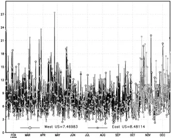
Hollingsworth, 2002). This is due mostly to improvements in the models and in the method whereby atmospheric ob-servations are incorporated into the initial conditions of the models, a process known as data assimilation (Daley, 1993; Kalnay, 2002). Most operational centers use a method called 3-Dimensional Variational data assimilation (3D-Var) to cre-ate the analysis that is used as an initial condition for the model. This method is a statistical interpolation of a short range forecast (typically 6 or 12 h) which serves as first guess or background, and the new observations. In this statistical interpolation, the background error covariance is maintained constant. That is, there is no accounting for the variations of the atmospheric state and consequent day-to-day variability of the background error covariance of forecasts from those states. These errors, not accounted by the fixed state of the background covariance matrix, are hereafter referred to as the “errors of the day”. The importance of the “errors of the day” can be seen in Fig. 1. Plotted is the root mean square analysis increment for the NCEP 50 year reanalysis during 1996, over two data-rich regions: the western (open circles) and eastern (gray dots) portions of the US. The average analysis incre-ment (the correction introduced by the new observations) is about 8 m at 500 hPa, but it varies widely from day-to-day, between low values of less than 3 m to high values over 20 m. There are several methods that try to account for the “er-rors of the day” in the forecast error covariance, including 4D-Var, Kalman Filtering, ensemble Kalman Filtering and the method of representers (e.g. Klinker et al., 2000; Ben-nett et al., 1996; Houtekamer and Mitchell, 1998; Hamill and Snyder, 2000). Unfortunately, these methods are com-putationally very expensive, and can only be implemented with substantial short-cuts, such as the use of a reduced rank background error covariance matrix in Kalman Filtering and lower model resolution in 4D-Var.
Fig. 1.Root mean square analysis increment in the 500 mb geopo-tential height for the NCEP 50 year reanalysis during 1996 over the western (open circles) and eastern (gray dots) portions of the US, courtesy of B. Kistler.
of this argument, a 3D-variational data assimilation scheme for a quasi-geostrophic channel model described in Morss (1998) and Rotunno and Bao (1996) is used to study the structure of the background error and its relationship to the corresponding bred vectors. The purpose of this paper is to test the extent to which bred vectors describe the shape of the “errors of the day”, and therefore could be used to include their effect in data assimilation, for example by augmenting the constant forecast error covariance used in 3D-Var with bred vectors (Corazza et al., 2002) or by performing an effi-cient local ensemble Kalman Filtering (Ott et al., 2002).
In Sect. 2, the quasi-geostrophic model and data assimila-tion system are reviewed and the method used to create bred vectors is presented. In Sect. 3 we first discuss the proper-ties of the bred vectors and present qualitative comparisons of their structure with the background “errors of the day” for a single case. In Sect. 4 we present statistics that summarize the results over many cases. A summary and conclusions are presented in Sect. 5.
2 Experimental set-up
The numerical model is a non-linear quasi-geostrophic mid-latitude flow in a channel discretized by finite differences both in horizontal and vertical directions (Rotunno and Bao, 1996; Morss, 1998; Morss et al., 2001). Each level consists of a grid of 64 longitude and 32 latitude points with a grid size of roughly 250 km in both zonal and meridional direc-tions. The model has seven levels, with five interior levels de-scribing the evolution of potential vorticity; while potential temperature is represented at the upper and the lower bound-aries. Horizontal diffusion is assumed to be proportional to
(a)
(b)
Fig. 2. Horizontal distribution of the rawinsonde locations for(a)
the 16 stations experiments and(b)the 32 stations experiments.
the squared Laplacian, and the model is forced by relaxation to a zonal mean state (Hoskins and West, 1979).
As in Morss (1998) and Hamill et al. (2000), we chose a single model integration as the “true” evolution of the model atmosphere. “Rawinsonde observations” are generated ev-ery 12 h by randomly perturbing the true state at fixed obser-vation locations (which were randomly chosen at initializa-tion). Two different resolutions for the observation network (16 and 32 locations, respectively) have been used based on Morss (1998) results that indicate that these numbers of sta-tions are representative of a low and medium density observ-ing network, respectively. In Figs. 2a and b the observation locations for the two cases are shown. In order to avoid errors due to interpolation processes, measurements are taken at the model grid points. For every rawinsonde, values for temper-atureT and horizontal components of wind velocityu and
v are simulated for all the seven layers of the model. The random noise to generate the observation errors is consistent using an observation-error covariance matrix which is set to zero except for variances and vertical covariances. The ver-tical correlation values are obtained by adapting the rawin-sonde variances given in Parrish and Derber (1992) and using the vertical correlations given in Eq. (3.19) from Bergman (1979) (Morss, 1998).
al-(a)
(b)
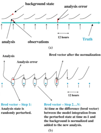
Fig. 3. (a)Schematic of the analysis cycle used in the system. Anal-ysis times are indicated by the short vertical arrows.(b)Schematic of the method used for the generation of the bred vectors.
gorithm similar to the operational Spectral Statistical Inter-polation (SSI) at NCEP (Parrish and Derber, 1992), which is a 3-D Var data assimilation scheme. In our experiments the same model is used for generating the truth and the forecasts, an approach known as a perfect model scenario (Fig. 3a). Be-cause this is a simulation system in which the truth is known, it allows for the explicit computation of the analysis and background errors. The background-error covariance ma-trixBis computed with the “NMC method”, deriving it from an ensemble of forecast differences, and assuming thatBis fixed in time and diagonal in horizontal spectral coordinates (as in Parrish and Derber, 1992). Moreover separate horizon-tal and vertical structures and simple vertical correlations are assumed. See Morss (1998) for more details on the implica-tions of these assumpimplica-tions and for a complete description of the implementation of the Data Assimilation System.
We compute k bred vectors in a manner similar to the procedure used in the ensemble forecasting systems at the National Centers for Environmental Prediction (Toth and Kalnay, 1993, 1997). The outline of the procedure is (Fig. 3b: (a)k random fields are added to the analysis; (b) the model is integrated for 12 h for each of thek perturbed fields; (c) the difference between each of the k perturbed integrations and the background 12 h forecast is uniformly scaled down so that the root mean square of the perturbation
is equal to the average squared analysis error at level three; (d) thekrescaled fields are then added to the new analysis and the steps (b) through (d) are repeated.
3 Characteristics of the bred vectors
Toth and Kalnay (1993, 1997) developed the breeding method to mimic in a simple way the data assimilation cy-cle, as suggested by a comparison of Figs. 3a and b. In an optimal sequential data assimilation scheme, the analysis er-ror covariance is given by the forecast erer-ror covariance mul-tiplied by a matrix [I−KH], the identity matrix minus the product of the effective filter gain and the observational op-erator (e.g. Ide et al., 1997). In breeding, this matrix is re-placed by the identity times a constant scalar representing the inverse of the global growth rate of the bred vector dur-ing the interval between rescaldur-ings. Kalnay and Toth (1994) conjectured that because of this similarity between the con-struction of the bred vectors and the data assimilation system both the background errors and the bred vectors would have similar local structures. In a perfect data assimilation system that accounts exactly for the errors of the day the conjecture may not be valid. For imperfect systems such as 3D-Var, if the background errors dominate the analysis errors, the con-jecture is more plausible, but it needs to be experimentally verified, and a simulation system provides the best tool for this purpose.
In this section we qualitatively explore this conjecture and other issues related to the robustness and representativeness of the bred vectors after a finite transient. More quantitative results based on a local analysis and statistical comparisons with surrogate experiments are presented in Sect. 4.
(a) (b)
(c) (d)
(e) (f)
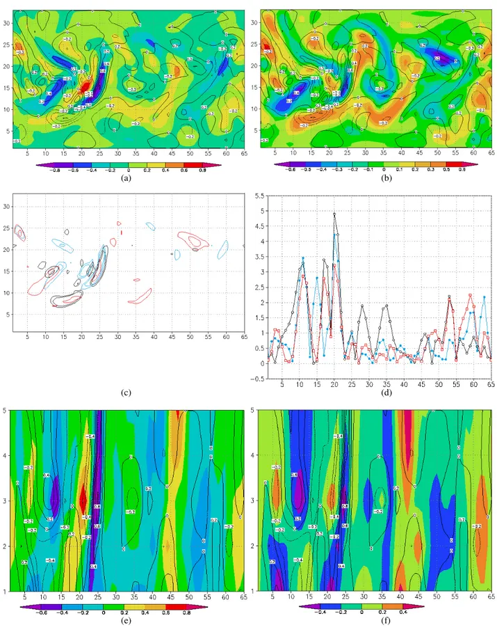
Fig. 5.Background error (contour) and a bred vector (color shaded) obtained with a breeding cycle based on the truth. The figure should be compared with Figs. 4a and b where the breeding cycle is based on the analysis.
with large amplitudes. The conclusions shown for the hori-zontal structure are equally valid for the vertical structure. In the examples shown in Figs. 4e and f the structure of the er-ror in the potential vorticity over most of the domain is well described by the bred vectors; nevertheless, in some areas it is possible to see secondary maxima in the bred vectors that do not correspond to any signal in the background error and vice versa.
3.1 Sensitivity to the details of the background flow It has been questioned in the past whether bred vectors com-puted using the analysis (which is only an estimate of the truth) are representative of the bred vectors that would be ob-tained if they were computed as perturbations of the “true” atmosphere. The results for the quasi-geostrophic system (Fig. 4) show that bred vectors obtained from the analysis are indeed very similar to those obtained from the truth. More-over, these results are valid for both low observational den-sity (Fig. 4) and at higher observation denden-sity (Fig. 6). In Fig. 6 level 3 potential vorticity from the bred vectors num-ber 1 and 5 and the background error are shown for the 32 stations simulation. As in the case of lower observational density, there is a good correspondence between the fields, and the structure of both the background error and the bred vector are similar to those obtained for the 16 observations simulation. This suggests that the analysis provides suffi-ciently close “shadowing” of the true atmosphere, and that the bred vectors depend on the instabilities of the large scale flow-of-the-day, rather than on the smaller scales details. 3.2 Finite time convergence
Toth and Kalnay (1993, 1997) observed for the operational global model of NCEP that it took only a transient period of few days for the randomly initialized bred vectors to develop well organized spatial structures in the mid-latitudes. This has been confirmed with the quasi-geostrophic model sys-tem: 3–5 days after initiating the breeding process with
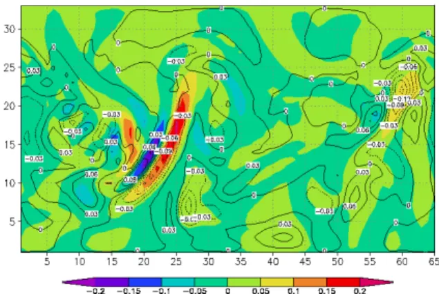
ran-dom perturbations, the bred vector growth rates attain their typical asymptotic range of values, and the bred vectors de-velop structures similar to the background errors. This is in good agreement with the results of Reynolds and Errico (1999), who computed finite time estimates of the Lyapunov vector in a quasi-geostrophic atmosphere on the sphere (here the growth over an analysis period is taken as the inverse of the rescaling factor employed for the bred vector at the anal-ysis time). This is shown in Fig. 7, which compares a bred vector (color shaded) and the background error (contours) five days after initiating the breeding process, and in Fig. 12, in the next section, which shows the rate at which conver-gence takes place.
3.3 Robustness with respect to the choice of norm
Because of their close relationship with leading Lyapunov vectors (Legras and Vautard, 1996; Szunyogh et al., 1997; Trevisan and Pancotti, 1998), bred vectors are expected to be insensitive to the choice of norm used to define the growth and rescaling. Figures 6 and 8 compare bred vectors obtained using a potential enstrophy (vorticity squared) norm,
k1q k= v u u t 1 N N X
i=1
(1q)2i ,
where(1q)iis the difference in potential vorticity at the con-sidered grid point i andN is the number of points, and a stream function norm,
k1ψk= v u u t 1 N N X
i=1
(1ψ )2i ,
where(1ψ )i is the difference in streamfunction at the grid pointi. Bred vectors obtained with both norms show a sim-ilar shape and relationship to the background error. This al-lows us to present our results only for the potential vorticity norm without losing generality in the conclusions.
These results are in contrast with singular vectors, which are extremely sensitive to the choice of norm. Palmer et al. (1998) and Snyder and Joly (1998) have shown that singular vectors obtained with a squared streamfunction norm have a horizontal scale much smaller than that obtained using an en-strophy norm, and those obtained with an energy norm have intermediate scales.
4 Local analysis of the subspace of the bred vectors and its relationship to the background error
In this section we present a local analysis of the bred vec-tors that allows a quantitative comparison of the relationship between bred vectors and the background error.
(a) (b)
(c) (d)
Fig. 6. (a)and(b)Two randomly chosen bred vectors for a medium density observing network (32 rawinsondes) (color shaded). Contours represent the corresponding background error. (c)vertical cross-section of the same vectors in (a) (y = 10). (d)same as Fig. 4d for the vectors represented in Figs. 6a and b [y=10].
method. For every grid point a surrounding domain of 25 grid points (5×5) – the local domain – is considered. For every bred vector and every grid point, we consider the 25 dimensional vector composed of the values of potential vor-ticity over the grid points of the local domain, which we refer to as a local bred vector. If there arekbred vectors, then at any point there arekcorresponding local bred vectors (in this sectionk≤25). We are interested in the degree of linear in-dependence of the local bred vectors. That is, we want to determine a quantitative measure of the effective dimension-ality of the subspace spanned by theklocal bred vectors.
To do this Patil et al. (2001) use principal component anal-ysis (Scheick, 1997) and define the bred vector dimension (BV-dimension) as:
9(σ1, σ2, . . . , σk)=
Pk i=1σi
2
Pk i=1σi2
,
whereσi, i = 1, . . . k are the singular values of thek×k
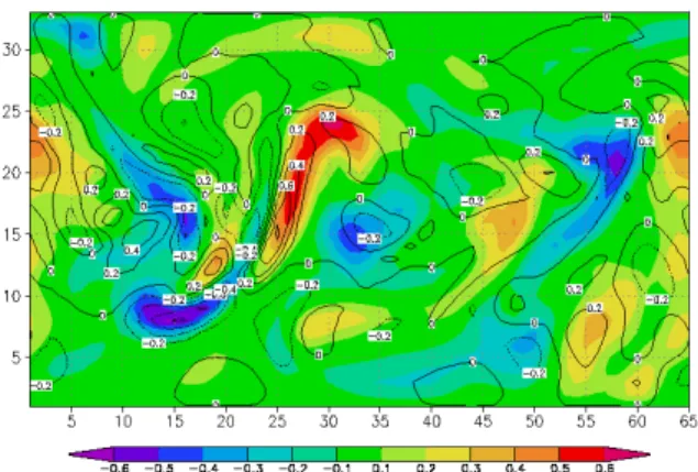
vec-Fig. 7.A bred vector (color shaded) and background error (contour) in potential vorticity at midlevel after 5 days from its initialization using the potential vorticity norm for rescaling.
tors needed to explain a certain level of variance, it has the advantage that, unlike explained variance, it is insensitive to the selection of an arbitrary threshold.
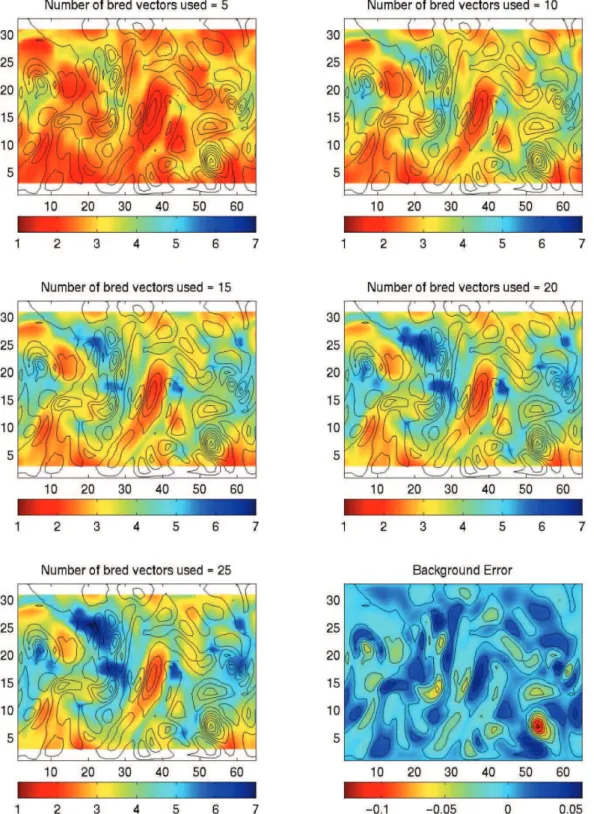
In our case we found that for k = 10 the local dimen-sion of this subspace is always smaller than about 5, and that there are areas where the dimensionality is much lower (less than 3). In Fig. 9 an example of the bred vector dimension is shown for the midlevel potential vorticity using different numbers of bred vectors. It is seen that increasing the number of bred vectors beyond 10 yields only a small spatial changes in the BV-dimension, especially in the regions of low dimen-sionality. This indicates that the results obtained with the local analysis with a set of 10 bred vectors can be considered representative of larger numbers of bred vectors in regions of low dimensionality. A more detailed analysis can be found in Patil (2001).
Figure 10a shows a scatter plot with the BV-dimension obtained at every grid point using 10 bred vectors during a period of 90 days, versus the background error squared valid at the same point in space and time. The same plot is made for the BV-dimension using 10 surrogates (Theiler et al., 1992) of the bred vectors, i.e. bred vectors correspond-ing to randomly chosen times that are at least 10 days away from each other and from the background error, so as to re-move any temporal correlation. The minimum and maximum BV-dimensions obtained on a daily basis with the real bred vectors has a mean of 1.4 and 3.7, respectively, whereas for surrogate vectors these values are about 4.2 and 7.5, respec-tively. The average BV-dimension of the surrogates, about 5.5, is low compared to the total subspace, but much larger than that obtained with bred vectors valid at the same time, which is 2.6. An analysis similar to that presented in Ta-ble 1 shows that (unlike explained variance), there is no sig-nificant dependence of the BV-dimension on the size of the background error.
Since bred vectors are computed using a finite time, finite amplitude extension to the method used to compute leading Lyapunov vectors, it might be expected that they should all converge to a single leading bred vector. However this is not
Fig. 8. Same as Figs. 6a or b but with the bred vector obtained using a streamfunction norm. Note that in Fig. 6 the bred vectors were obtained using potential vorticity norm.
the case in the operational global forecast models or even for the simpler quasi-geostrophic model (Fig. 10a). This is due to nonlinear forcing and to the fact that in these com-plex systems several instabilities can coexist in different lo-cations (Kalnay et al., 2002). As a result the bred vectors remain globally different, but in regions in which the back-ground flow is locally unstable, they collapse into a lower-dimensional subspace represented by the dominant local in-stabilities.
4.2 Similarity between the local structure of bred vectors and background errors
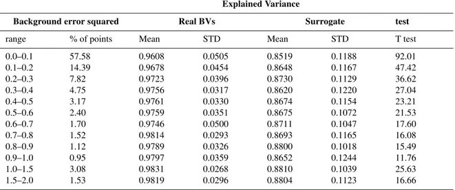
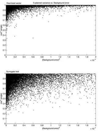
In Sect. 3 we showed qualitative instantaneous similarity be-tween individual bred vectors and the background errors. This similarity can be quantified by computing the extent to which the background error lies within the subspace of the bred vectors. At each point, for 90 days, we computed the local angle between the background error and the subspace of bred vectors, and therefore found that in most grid points the angle is less than 10◦, corresponding to an explained vari-ance (e.g. Wilks, 1995) of more than 0.97. Figure 11a shows a scatterplot of the explained variance (square of the angle between the background error and the subspace of 10 bred vectors) as a function of the background error size for a pe-riod of 90 days. It clearly shows that the background error is mostly confined to the subspace of the bred vectors and therefore that it is in principle possible to effectively correct the background state by simply moving it toward the obser-vations within this subspace. Figure 11b shows the same scatterplot but for the surrogate bred vectors corresponding to 10 randomly chosen times, as in Fig. 10b. Table 1 sum-marizes the statistics for the explained variance. The t-test corresponds to the null hypothesis that the real bred vectors and the surrogates explain the same variance, and shows that it should be rejected with very high significance.
Fig. 9. BV-dimension (5×5 local domains) obtained using different numbers of bred vectors (5–25 vectors). The contour lines show the background error (also shown in color shades in the bottom-right plot).
variance, much better that what a subspace of random vec-tors would do. This should not be surprising, because, by construction, the surrogates are representative of the statis-tically averaged subspace of bred vectors. The construction of the 3D-Var background error covariance using the “NMC method” (Parrish and Derber, 1992) is based on a subspace
Table 1.Comparison of the explained variance of the background error using real bred vectors and surrogates (bred vectors corresponding to randomly chosen times). The results are computed for every grid point over 90 days, and binned as a function of the square of the background error
Explained Variance
Background error squared Real BVs Surrogate test
range % of points Mean STD Mean STD T test
0.0–0.1 57.58 0.9608 0.0505 0.8519 0.1188 92.01
0.1–0.2 14.39 0.9678 0.0454 0.8648 0.1167 47.42
0.2–0.3 7.82 0.9723 0.0396 0.8730 0.1129 36.62
0.3–0.4 4.75 0.9756 0.0317 0.8620 0.1220 27.04
0.4–0.5 3.17 0.9761 0.0330 0.8674 0.1154 23.21
0.5–0.6 2.40 0.9759 0.0351 0.8675 0.1072 21.53
0.6–0.7 1.70 0.9746 0.0500 0.8711 0.1047 17.60
0.7–0.8 1.52 0.9814 0.0293 0.8693 0.1165 16.08
0.8–0.9 1.12 0.9789 0.0326 0.8800 0.1018 15.49
0.9–1.0 0.95 0.9797 0.0359 0.8652 0.1244 11.76
1.0–1.5 3.08 0.9831 0.0268 0.8810 0.1039 25.63
1.5–2.0 1.53 0.9819 0.0296 0.8804 0.1123 16.66
Fig. 10. BV-Dimension as a function of the background error squared, computed for 90 days over every grid point. (a)using 10 bred vectors corresponding to the same time as the background error.(b)using 10 surrogate bred vectors corresponding to random times.
shows the potential improvement that including the “errors of the day” could bring to the 3D-Var data assimilation.
Finally, in Fig. 12 we show the evolution of the average
ex-plained variance as a function of time for bred vectors started from initial random perturbations. It shows that the bred vec-tor subspace converges quickly, within 3–5 days, and that the results are robust in time. For the surrogates the explained variance does not change with time.
5 Discussion and conclusions
In this paper we have used a 3D-variational data assimilation scheme for a quasi-geostrophic channel model (Morss, 1998) to study the structure of the background error and its relation-ship to the corresponding bred vectors. By defining a model integration as the “true” evolution of the model atmosphere we were able to explicitly compute the background errors and make direct comparisons of these errors to bred vectors. We have observed that in the quasi-geostrophic simulation system, as in the operational data assimilation system, the background errors have a large day-to-day variability, which we have called “errors of the day”. The errors of the day tend to have periods of fast growth, resulting in large amplitudes intermittent in both space and in time.
We have obtained the following results:
– Convergence to well organized structures in the bred vectors occurs within a few (3–5) days (Sects. 3.2 and 4.2).
– Bred vectors obtained using normalizations based on the potential vorticity and on the streamfunction have very similar structures (Sect. 3.3).
Fig. 11. Explained variance (square of the cosine of the angle be-tween the background error and the space defined by the local vec-tors) as a function of the background error squared, computed for 90 days over every grid point.(a)using 10 bred vectors correspond-ing to the same time as the background error.(b)using 10 surrogate bred vectors corresponding to random times.
the bred vectors are not too sensitive to the details of the flow and that the errors themselves are more likely dependent on the large scale nature of the flow (at least in a perfect model assumption). Since the truth is not available in practice, this is important because it sug-gests that basing bred vectors on the analysis is not a significant limitation in operational systems.
– The bred vectors have spatial characteristics similar to those of the background “error of the day” (Figs. 4, 12). – Following Patil et al. (2001) we computed a measure of the space spanned by the bred vectors (BV-dimension). We found that the local dimension is much smaller than the number of bred vectors. Moreover, the information given by a set of ten bred vectors is not significantly different from that obtained using a larger number of vectors (Sect. 4).
– We also defined the local angle between the forecast er-ror and the subspace of bred vectors. When averaging over many cases, we found that in most of the model do-main the angle is confined to less than 10◦, with a mean explained variance of 96–98%, indicating that the back-ground error is mostly confined to the subspace of the bred vectors (Sect. 4.2). Larger angles (lower explained
Fig. 12. Evolution of the average explained variance as a function of time for bred vectors started from initial random perturbations (red dots) and for the surrogate (blue line).
variance) are only observed in regions where the back-ground error is small (Fig. 12).
– The explained variance of the forecast error using sur-rogate bred vectors (corresponding to random times) is also high, about 85%. We suggest that this reflects the reason why 3D-Var is quite successful even though it does not take into account the errors of the day, since the ”NMC method” used to construct the background error covariance is based on forecast differences related to bred vectors.
These results suggest that the bred vectors can indeed be useful in specifying the part of the background error covari-ance that corresponds to the “errors of the day”. We are currently developing computationally inexpensive methods to take advantage of this information. Preliminary results (Corazza et al., 2002) indicate a substantial improvement in the analysis errors and in the forecasts at a small computa-tional overhead. An economic local ensemble Kalman Fil-tering approach is described in Ott et al. (2002).
comments led to a major improvement in the paper. This research was supported by the W. M. Keck Fundation, NPOESS IPO (adap-tive targetting, grant SWA01005), NASA (AIRS data assimilation, STMD CG0127), Office of Naval Research, and National Science Fundation (award DMS0104087, grant no. 0104087).
References
Bennett, A. F., Chua, B. S., and Leslie, L. M.: Generalized inversion of a global NWP model, Meteor. Atmos. Phys., 60, 165–178, 1996.
Bergman, K. H.: Multivariate analysis of temperatures and winds using optimum interpolation, Mon. Wea. Rev., 107, 1423–1444, 1979.
Corazza, M., Kalnay, E., Patil, D. J., Ott, E., Yorke, J., Szunyogh, I., and Cai, M.: Use of the breeding technique in the estimation of the background error covariance matrix for a quasigeostrophic model, in AMS Symposium on Observations, Data Assimila-tion and Probabilistic PredicAssimila-tion, pp. 154–157, Orlando, Florida, 2002.
Daley, R.: Atmospheric data analysis, Cambridge University Press, New York, 1993.
Hamill, T. M. and Snyder, C.: A Hybrid Ensemble Kalman Filter-3D Variational Analysis Scheme, Mon. Wea. Rev., 128, 2905– 2919, 2000.
Hamill, T. M., Snyder, C., and Morss, R. E.: A Comparison of Prob-abilistic Forecasts from Bred, Singular-Vector and Perturbed Ob-servation Ensembles, Mon. Wea. Rev., 128, 1835–1851, 2000. Hoskins, B. J. and West, N. V.: Baroclinic waves and frontogenesis.
Part II: Uniform potential vorticity jet flows – Cold and warm fronts, J. Atmos. Sci., 36, 1663–1680, 1979.
Houtekamer, P. L. and Mitchell, H. L.: Data assimilation usin an ensemble Kalman filter technique, Mon. Wea. Rev., 126, 796– 811, 1998.
Ide, K., Courtier, P., Ghil, M., and Lorenc, A. C.: Unified notation for data assimilation: Operational, sequential, and variational, J. Meteor. Soc. Japan, 75(1B), 181–189, 1997.
Kalnay, E.: Atmospheric Modeling, Data Assimilation and Pre-dictability, Cambridge University Press, 340 pp., 2002. Kalnay, E. and Toth, Z.: Removing growing errors in the analysis
cycle, in: Tenth Conference on Numerical Weather Prediction, pp. 212–215, Amer. Meteor. Soc., 1994.
Kalnay, E., Lord, E. S., and McPherson, R.: Maturity of Operational Numerical Weather Prediction: the Medium Range, Bull. Amer. Meteor. Soc., 79, 864–875, 1998.
Kalnay, E., Corazza, M., and Cai, M.: Are bred vectors the same as Lyapunov vectors?, in: AMS Symposium on Observations, Data Assimilation and Probabilistic Prediction, pp. 173–177, Orlando, Florida, 2002.
Klinker, E., Rabier, F., Kelly, G., and Mahfouf, J.-F.: The ECMWF operational implementation of four-dimensional variational as-similation, iii: Experimental results and diagnostics with oper-ational configuration, Quart. J. Roy. Meteor. Soc., 126, 1191, 2000.
Legras, B. and Vautard, R.: A guide to Liapunov vectors, in Pro-ceedings 1995 ECMWF Seminar on Predictability, Vol I, pp. 143–156, 1996.
Morss, R. E., Adaptive observations: Idealized sampling strategies for improving numerical weather prediction, Ph.D. thesis, Mas-sachusetts Institute of Technology, 225 pp., 1998.
Morss, R. E., Emanuel, K. A., and Snyder, C.: Idealized Adaptive Observation Strategies for Improving Numerical Weather Pre-diction, J. Atmos. Sci., 58, 210–234, 2001.
Ott, E., Hunt, B. R., Szunyogh, I., Corazza, M., Kalnay, E., Patil, D. J., and Yorke, J. E.: Exploiting low-dimensionality of the atmospheric dynamics for efficient ensemble kalman filtering, http://arXiv:physics/0203058\/, 2002.
Palmer, T. N., Gelaro, R., Barkmeijer, J., and Buizza, R.: Singular vectors, metrics and adaptive observations, J. Atmos. Sci., 55, 633–653, 1998.
Parrish, D. F. and Derber, J. D.: The National Meteorological Cen-ter spectral statistical inCen-terpolation analysis system, Mon. Wea. Rev., 120, 1747–1763, 1992.
Patil, D. J.: Applications of chaotic dynamics to weather forecast-ing, Ph.D. thesis, University of Maryland, 2001.
Patil, D. J. S., Hunt, B. R., Kalnay, E., Yorke, J. A., and Ott, E.: Lo-cal Low Dimensionality of Atmospheric Dynamics, Phys. Rev. Lett., 86, 5878, 2001.
Reynolds, C. A. and Errico, R. M.: Convergence of singular vec-tors toward Lyapunov vecvec-tors, Mon. Wea. Rev., 127, 2309–2323, 1999.
Reynolds, C. A., Webster, P. J., and Kalnay, E.: Random error growth in NMC’s global forecasts, Mon. Wea. Rev., 122, 1281– 1305, 1994.
Rotunno, R. and Bao, J. W.: A case study of cyclogenesis using a model hierarchy, Mon. Wea. Rev., 124, 1051–1066, 1996. Scheick, J. T.: Linear Algebra with Applications, McGraw Hill,
1997.
Simmons, A. J. and Hollingsworth, A.: Some aspects of the im-provement in skill of numerical weather prediction, Quart. J. Roy. Meteor. Soc., 128, 2002.
Snyder, C. and Joly, A.: Development of perturbations within a growing baroclinic wave, Quart. J. Roy. Meteor. Soc., 124, 1961– 1983, 1998.
Szunyogh, I., Kalnay, E., and Toth, Z.: A comparison of Lyapunov and optimal vectors in a low resolution GCM, Tellus, 49A, 200– 227, 1997.
Szunyogh, I., Toth, Z., Morss, R. E., Majumdar, S. J., Etherton, B. J., and Bishop, C. H.: The Effect of Targeted Dropsonde Ob-servations during the 1999 Winter Storm Reconnaissance Pro-gram, Mon. Wea. Rev., 128, 3520–3537, 2000.
Theiler, J., Eubank, S., Longtin, A., Galdrikian, B., and Farmer, J. D.: Testing for nonlinearity in time series: the method of sur-rogate data, Physica D, 58, 77–94, 1992.
Toth, Z. and Kalnay, E.: Ensemble forecasting at NMC: the genera-tion of perturbagenera-tions, Bull. Amer. Meteor. Soc., 74, 2317–2330, 1993.
Toth, Z. and Kalnay, E.: Ensemble forecasting at NCEP: the breed-ing method, Mon. Wea. Rev., 125, 3297–3318, 1997.
Trevisan, A. and Pancotti, F.: Periodic orbits, Lyapunov vectors and singular vectors in the Lorenz system, J. Atmos. Sci., 55, 390– 398, 1998.