www.atmos-meas-tech.net/7/279/2014/ doi:10.5194/amt-7-279-2014
© Author(s) 2014. CC Attribution 3.0 License.
Atmospheric
Measurement
Techniques
Application of mobile aerosol and trace gas measurements for the
investigation of megacity air pollution emissions: the Paris
metropolitan area
S.-L. von der Weiden-Reinmüller1, F. Drewnick1, M. Crippa2,*, A. S. H. Prévôt2, F. Meleux3, U. Baltensperger2, M. Beekmann4, and S. Borrmann1,5
1Particle Chemistry Department, Max Planck Institute for Chemistry, Mainz, Germany 2Laboratory of Atmospheric Chemistry, Paul Scherrer Institute, Villigen, Switzerland 3Institut National de l‘Environnement Industriel et des Risques, Verneuil en Halatte, France
4Laboratoire inter-universitaire des Systèmes Atmosphériques, UMR7583 – CNRS, Université Paris Est Créteil et Université
Paris Diderot, France
5Institute of Physics of the Atmosphere, Johannes Gutenberg University Mainz, Mainz, Germany
*now at: European Commission Joint Research Centre, Institute for Environment and Sustainability, Ispra, Italy
Correspondence to:F. Drewnick (frank.drewnick@mpic.de)
Received: 6 August 2013 – Published in Atmos. Meas. Tech. Discuss.: 22 August 2013 Revised: 22 November 2013 – Accepted: 9 December 2013 – Published: 28 January 2014
Abstract.For the investigation of megacity emission devel-opment and the impact outside the source region, mobile aerosol and trace gas measurements were carried out in the Paris metropolitan area between 1 July and 31 July 2009 (summer conditions) and 15 January and 15 February 2010 (winter conditions) in the framework of the European Union FP7 MEGAPOLI project. Two mobile laboratories, MoLa and MOSQUITA, were deployed, and here an overview of these measurements and an investigation of the applicabil-ity of such measurements for the analysis of megacapplicabil-ity emis-sions are presented. Both laboratories measured physical and chemical properties of fine and ultrafine aerosol parti-cles as well as gas phase constituents of relevance for ur-ban pollution scenarios. The applied measurement strate-gies include cross-section measurements for the investigation of plume structure and quasi-Lagrangian measurements ax-ially along the flow of the city’s pollution plume to study plume aging processes. Results of intercomparison mea-surements between the two mobile laboratories represent the adopted data quality assurance procedures. Most of the compared measurement devices show sufficient agreement for combined data analysis. For the removal of data con-taminated by local pollution emissions a video tape analy-sis method was applied. Analyanaly-sis tools like positive matrix
factorization and peak integration by key analysis applied to high-resolution time-of-flight aerosol mass spectrometer data are used for in-depth data analysis of the organic par-ticulate matter. Several examples, including a combination of MoLa and MOSQUITA measurements on a cross section through the Paris emission plume, are provided to demon-strate how such mobile measurements can be used to inves-tigate the emissions of a megacity. A critical discussion of advantages and limitations of mobile measurements for the investigation of megacity emissions completes this work.
1 Introduction
will classify as megacities (United Nations, 2012). Along with major challenges as urban planning, industrial devel-opment and transportation these intense pollution hot-spots cause a number of scientific questions concerning their in-fluence on local and regional air quality, with its impact on human health, flora and fauna as well as atmospheric chem-istry and climate (e.g. Kunkel et al., 2012).
In Europe the metropolitan areas of London, Paris, the Rhine-Ruhr and the Po valley regions, Moscow and Istan-bul are classified as megacities. Within the framework of the European Union FP7 MEGAPOLI project (Megacities: Emissions, urban, regional and Global Atmospheric POL-lution and climate effects, and Integrated tools for assess-ment and mitigation; MEGAPOLI Project, 2013) two major field campaigns were carried out in the greater Paris region in summer 2009 and winter 2010. The focus of these mea-surement campaigns was to characterise the Paris emission plume with respect to trace gases (e.g. O3, SO2, NOx, CO2)
and aerosol particles in the size range from a few nanome-ters to several micromenanome-ters including chemical composition. The overall goal was to assess its impact on the local and regional air quality and to investigate aerosol transformation processes within this plume as it travels away from its source. This includes the influence of meteorology on the emission plume due to different environmental conditions in summer and winter.
Typically, aerosol and trace gas measurements are per-formed at stationary sites what leads to a strong spatial lim-itation of the data and dependency on peculiarities of the chosen location. Especially for the investigation of emissions from spatially extended aerosol sources like cities and forma-tion and transformaforma-tion of particles during transport, staforma-tion- station-ary measurements are only suitable to a limited extent. For this purpose, in the past few years several ground-based mo-bile laboratories equipped with high-time resolution instru-mentation have been developed which allow measurements with large spatial flexibility (Bukowiecki et al., 2002; Kolb et al., 2004; Pirjola et al., 2004; Drewnick et al., 2012). These ground-based mobile laboratories installed on vehicles are an expedient addition to research aircraft and laboratories in-stalled on ships.
Here we focus on mobile ground-based measurements of aerosol and trace gas characteristics that were carried out during both campaigns by two research groups with two dif-ferent mobile aerosol laboratories. These mobile measure-ments were embedded in a network of stationary ground-based, additional mobile ground-based remote sensing and aircraft measurements, satellite observations and local, re-gional and global modelling (Beekmann et al., 2014). To in-tegrate the presented measurements in a greater context of ur-ban pollution investigations (e.g. in Barcelona, Beijing, Mex-ico City, Nashville, Paris, West Midlands, UK) we refer to the comprehensive number of publications focused on this topic (e.g. Nunnermacker et al., 1998; McMurry, 2000; Raga et al., 2001; Seakins et al., 2002; Harrison et al., 2006; Gros
et al., 2007; Pey et al., 2008; Elanskii et al., 2010; Mohr et al., 2012; Crippa et al., 2013; Freutel et al., 2013).
The measured parameters of both mobile laboratories in-clude concentrations of gas phase O3, NOxand CO2, aerosol
particle number concentration, size distribution and chemi-cal composition as well as meteorologichemi-cal parameters (wind direction, relative humidity, pressure and temperature). For the measurement of the sub-micron particle chemical com-position on-line measurement devices such as the aerosol mass spectrometer (Jayne et al., 2000; DeCarlo et al., 2006; Lanz et al., 2010) have been deployed and adopted for the mobile measurements. In combination with complex analy-sis tools as positive matrix factorization (PMF) (Paatero and Tapper, 1994; Paatero, 1997; Lanz et al., 2007; Ulbrich et al., 2009) and peak integration by key analysis (PIKA) (ToF-AMS Analysis Software Homepage, 2013) a large amount of information can be obtained about aerosol chemical compo-sition (Zhang et al., 2005; Canagaratna et al., 2007; Sun et al., 2010; Zhang et al., 2011). The measurement of carbon dioxide, ozone and nitrogen oxides together with meteoro-logical parameters is needed for numerical simulation of the urban atmospheric chemistry (e.g. Fenger, 1999; Akimoto, 2003; Crutzen, 2004; Gurjar and Lelieveld, 2005).
The purpose of this paper is to discuss the general ap-plicability of the developed and deployed measurement and analysis strategies for urban emission investigations using the MEGAPOLI data base as example. In Sect. 2 we pro-vide an overview of the MEGAPOLI field campaigns and describe the two mobile laboratories including specification and intercomparison of the on-board instruments, as well as different measurement strategies. A general overview of the advanced data preparation for analysis completes this sec-tion. In Sect. 3 four examples of mobile measurements are presented that investigate the differences between long-range transported and locally produced pollution. A combination of data from both mobile laboratories allows a detailed view of the spatial structure of the emission plume. Axial mea-surement trips show the spatial extent of the emission plume, while a final example of stationary measurements at various locations around the city illustrates the influence of the Paris emission plume on local air quality. These measurement ex-amples demonstrate the successful application of the individ-ual measurement strategies. Section 4 provides a critical dis-cussion of possibilities, challenges and limitations of mobile measurements.
2 Methods
2.1 MEGAPOLI field campaigns
An additional goal is the quantification of feedbacks between megacity emissions, air quality, local and regional climate, and global climate change. Based on new findings improved, integrated tools are to be developed and implemented in ex-isting air quality models to assess the impacts of air pollu-tion from megacities on regional and global air quality and climate and to evaluate the effectiveness of mitigation strate-gies.
MEGAPOLI field campaigns: two major field campaigns took place in the greater Paris region in France, which is clas-sified as megacity with currently about 10.6 million inhabi-tants (United Nations, 2012). The greater Paris metropoli-tan area, defined as the territory with high residential den-sity and additional surrounding areas that are also influ-enced by the city, for example by frequent transport or road linkages (United Nations, 2012), has actually a population of more than 12 million inhabitants (Aire urbaine, 2013). The summer measurement period was carried out between 1 July and 31 July 2009, the winter field campaign between 15 January and 15 February 2010. The main objective of these field measurements was to characterise and quantify sources of primary and secondary aerosol in and around a large agglomeration and to investigate its evolution and im-pacts on local and regional air quality as well as atmospheric chemistry in the megacity emission plume. Three ground-based stationary measurement sites were operated – two sub-urb and one downtown sites (for details see MEGAPOLI project, 2013; Freutel et al., 2013; Crippa et al., 2013). Mo-bile measurements were carried out by a research aircraft (applying an ATR42 in summer and a Piper Aztec in winter, SAFIRE, 2013), remote-sensing mobile laboratories (DOAS instrument operated on top of a regular passenger vehicle, a LIDAR instrument installed on a pick-up truck, Royer et al., 2011) and the two mobile aerosol research laboratories MoLa and MOSQUITA. These mobile laboratories measured while driving through atmospheric background and emis-sion plume influenced air masses, carried out several station-ary measurements at various places in and around Paris and were also used for intercomparison studies with the station-ary measurement sites and the research aircraft.
2.2 Mobile laboratories and on-board instrumentation
2.2.1 Mobile laboratory “MoLa”
Platform: the Max Planck Institute for Chemistry in Mainz, Germany, developed a compact Mobile aerosol research Lab-oratory (“MoLa”) based on a Ford Transit delivery vehicle for stationary and mobile measurements of aerosol phys-ical and chemphys-ical properties and trace gas concentrations (Drewnick et al., 2012). The main inlet system for mobile measurements is located above the driver’s cabin at a height of approximately 2.2 m and it is equipped with a nozzle op-timised for an average driving velocity of about 50 km h−1. Stationary measurements are performed using an extendable
inlet (up to 10 m) on the roof of the vehicle for aerosol sampling. A specific feature of the MoLa aerosol inlet sys-tem is its optimisation for minimal sampling and transport losses using the Particle Loss Calculator (von der Weiden et al., 2009). The residence time of the aerosol during its way through the inlet system to the individual instruments was measured and calculated for sampling time correction and the occurring – but negligible – particle losses were quanti-fied (see Sect. 2.3 and Drewnick et al., 2012).
Instrumentation: Table 1 provides detailed information on the deployed instruments. During both field campaigns MoLa was equipped with a High-Resolution Time-of-Flight Aerosol Mass Spectrometer (HR-ToF-AMS; DeCarlo et al., 2006) to measure size-resolved mass concentrations of non-refractory species approximately in the PM1size range.
Ad-ditionally, black carbon and particle-bound polycyclic aro-matic hydrocarbon (PAH) mass concentrations were mea-sured to achieve detailed chemical information about total PM1particle composition, including most species found in
the sub-micron aerosol. The aerosol total number concentra-tion was measured as well as aerosol particle size distribu-tions applying three different techniques (electrical mobil-ity, aerodynamic sizing, light scattering). The detected trace gases include O3, SO2, NO, NO2, CO, CO2 and H2O.
Me-teorological parameters like wind direction and speed, ambi-ent pressure, temperature, relative humidity and precipitation were recorded as well as GPS vehicle position and environ-mental conditions (e.g. traffic situation) using a webcam.
2.2.2 Mobile laboratory “MOSQUITA”
Platform: the Paul Scherrer Institute in Villigen, Switzer-land, developed a mobile aerosol and trace gas laboratory (Measurements Of Spatial QUantitative Imissions of Trace gases and Aerosols: “MOSQUITA”; Bukowiecki et al., 2002; Weimer et al., 2009; Mohr et al., 2011; Mobile Laboratory MOSQUITA, 2013), which utilises an IVECO Turbo Daily Transporter as platform. The main aerosol inlet is located at a height of 3.2 m in the front part of the vehicle allowing for isokinetic sampling at a driving velocity of 50 km h−1.
Instrumentation: Table 2 shows the equipment used in MOSQUITA. PM1 particle chemical composition was
ob-tained from a HR-ToF-AMS and additional black carbon mass concentration measurements. Aerosol particle concen-trations were measured in total as well as size-resolved ap-plying different techniques in summer (electrical mobility) and winter (light scattering). The recorded trace gases are O3, NO, NO2, CO, CO2and H2O. Meteorological
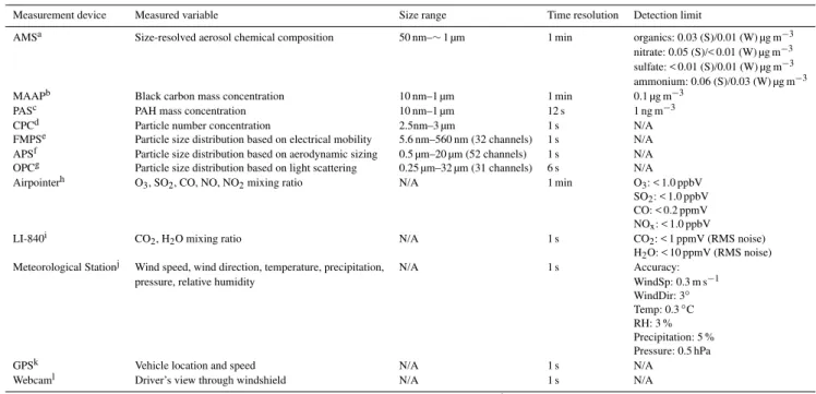
Table 1.Summary of measurement devices – including information about measured variables, size range, time resolution and detection limit – installed in the mobile laboratory MoLa (Max Planck Institute for Chemistry) during the summer and winter MEGAPOLI field campaigns. AMS detection limits (using the method described in Drewnick et al., 2009) were calculated for summer (S) and winter field campaign (W) separately, because the AMS detection limit can change over time.
Measurement device Measured variable Size range Time resolution Detection limit
AMSa Size-resolved aerosol chemical composition 50 nm–∼1 µm 1 min organics: 0.03 (S)/0.01 (W) µg m−3
nitrate: 0.05 (S)/< 0.01 (W) µg m−3 sulfate: < 0.01 (S)/0.01 (W) µg m−3
ammonium: 0.06 (S)/0.03 (W) µg m−3 MAAPb Black carbon mass concentration 10 nm–1 µm 1 min 0.1 µg m−3
PASc PAH mass concentration 10 nm–1 µm 12 s 1 ng m−3
CPCd Particle number concentration 2.5nm–3 µm 1 s N/A
FMPSe Particle size distribution based on electrical mobility 5.6 nm–560 nm (32 channels) 1 s N/A APSf Particle size distribution based on aerodynamic sizing 0.5 µm–20 µm (52 channels) 1 s N/A
OPCg Particle size distribution based on light scattering 0.25 µm–32 µm (31 channels) 6 s N/A Airpointerh O
3, SO2, CO, NO, NO2mixing ratio N/A 1 min O3: < 1.0 ppbV
SO2: < 1.0 ppbV
CO: < 0.2 ppmV NOx: < 1.0 ppbV
LI-840i CO2, H2O mixing ratio N/A 1 s CO2: < 1 ppmV (RMS noise)
H2O: < 10 ppmV (RMS noise) Meteorological Stationj Wind speed, wind direction, temperature, precipitation, N/A 1 s Accuracy:
pressure, relative humidity WindSp: 0.3 m s−1
WindDir: 3◦
Temp: 0.3◦C RH: 3 % Precipitation: 5 % Pressure: 0.5 hPa
GPSk Vehicle location and speed N/A 1 s N/A
Webcaml Driver’s view through windshield N/A 1 s N/A
aAerosol Mass Spectrometer (AMS), HR-ToF-AMS, Aerodyne Research, Inc., USA, (http://aerodyne.com, last access: 15 November 2013).bMulti-Angle Absorption Photometer (MAAP), Carusso/Model 5012 MAAP, Thermo Electron Corp., USA, (http://thermoscientific.com, last access: 15 November 2013).cPhotoelectric Aerosol Sensor (PAS), EcoChem Model PAS2000, Ansyco, Germany, (http://ansyco.de, last access: 15 November 2013). dCondensation Particle Counter (CPC), Model 3786, TSI, Inc., USA, (http://tsi.com, last access: 15 November 2013).eFast Mobility Particle Sizer Spectrometer (FMPS), Model 3091, TSI, Inc., USA.fAerodynamic Particle Sizer Spectrometer (APS), Model 3321, TSI, Inc., USA.gOptical Particle Counter (OPC), Model 1.109, Grimm Aerosoltechnik, Germany, (http://grimm-aerosol.com, last access: 15 November 2013).hAirpointer, Recordum Messtechnik GmbH, Austria, (http://www.recordum.com, last access: 15 November 2013).iLI-COR, Model LI-840, Corp., USA, (http://licor.com, last access: 15 November 2013).jModel WXT520, Vaisala, Finland, (http://vaisala.com, last access: 15 November 2013).kGarmin, GPSmap 278, Garmin Ltd., USA, (http://garmin.com, last access: 15 November 2013).lModel EDIMAX IC7000, Edimax Technology Co., Ltd., Taiwan, (http://edimax.com, last access: 15 November 2013).
2.2.3 Intercomparison of corresponding measurement
devices on MoLa and MOSQUITA
Intercomparison measurements were carried out several times during both field campaigns. Not only MoLa and MOSQUITA were compared, but also both mobile labora-tories with the other stationary ground-based measurement sites and the research aircraft. A detailed description of the results of these other intercomparison exercises can be found in Freutel et al. (2013) and Crippa et al. (2013).
For the two mobile laboratories the instruments (see Ta-bles 1 and 2) measuring the following parameters were com-pared in this study:
– Particle number size distribution (FMPS, UHSAS, APS, OPC),
– Particle number concentration (CPC3786, CPC3010s),
– Non-refractory chemical aerosol composition (two HR-ToF-AMS),
– Black Carbon mass concentration (two MAAP),
– CO2mixing ratio (LI-840, LI-7000),
– O3mixing ratio (Airpointer, Ozone monitor), and
– NOxmixing ratio (Airpointer, Luminox monitor).
CO mixing ratio was not compared, because due to issues with the MoLa instrument all measurements were below de-tection limit during both campaigns and thus were not used for further analysis. NO and NO2data are not available for
MOSQUITA during the intercomparisons due to instrumen-tal issues. The intercomparison of the MoLa weather param-eters showed excellent agreement with the meteorological parameters measured at the North-East suburb measurement site (Freutel et al., 2013).
Intercomparison time periods: the intercomparison time periods during the summer campaign were 11 July 2009 from 12:05:00 until 17:39:00 (at Pontoise airport) and 23 July 2009 from 11:22:00 until 19:00:00 (at the South-West suburb measurement site). The winter intercomparison took place on 9 February 2010 from 11:42:00 until 19:30:00 also at the South-West suburb measurement site. All given times are in local time. For details about the mentioned mea-surement sites we refer to the MEGAPOLI project’s website (MEGAPOLI Project, 2013) and Beekmann et al. (2014).
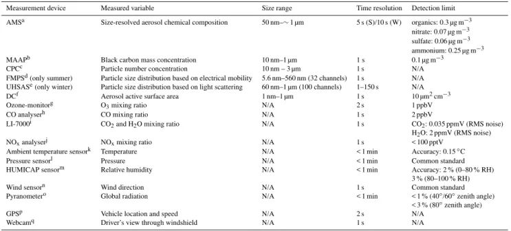
Table 2.Summary of measurement devices – including information about measured variables, size range, time resolution and detection limit – installed in the mobile laboratory MOSQUITA (Paul Scherrer Institute) during the summer and winter MEGAPOLI field campaigns. AMS detection limits were calculated and averaged for the two mobile measurements presented in this work (S = summer, W = winter).
Measurement device Measured variable Size range Time resolution Detection limit
AMSa Size-resolved aerosol chemical composition 50 nm–∼1 µm 5 s (S)/10 s (W) organics: 0.3 µg m−3
nitrate: 0.07 µg m−3 sulfate: 0.06 µg m−3
ammonium: 0.25 µg m−3
MAAPb Black carbon mass concentration 10 nm–1 µm 1 s 0.1 µg m−3
CPCc Particle number concentration 10 nm – 3 µm 1 s N/A
FMPSd(only summer) Particle size distribution based on electrical mobility 5.6 nm–560 nm (32 channels) 1 s N/A UHSASe(only winter) Particle size distribution based on light scattering 60 nm–1 µm (100 channels) 1–150 s N/A
DCf Aerosol active surface area 1 nm–1 µm 1 s 10 µm2cm−3
Ozone-monitorg O
3mixing ratio N/A 2 s 1 ppbV
CO analyserh CO mixing ratio N/A 1 s 2 ppbV
LI-7000i CO2and H2O mixing ratio N/A 1 s CO2: 0.035 ppmV (RMS noise)
H2O: 2 ppmV (RMS noise)
NOxanalyserj NOxmixing ratio N/A 1 s < 100 pptV
Ambient temperature sensork Temperature N/A < 1 min Accuracy: 0.15◦C
Pressure sensorl Pressure N/A < 1 min Common standard
HUMICAP sensorm Relative humidity N/A < 1 min Accuracy: 2 % (0–80 % RH)
3 % (80–100 % RH)
Wind sensorn Wind direction N/A 1 s Common standard
Pyranometero Global radiation N/A < 1 min < 1 % (40◦/60◦zenith angle) < 3 % (80◦zenith angle)
GPSp Vehicle location and speed N/A 2 s N/A
Webcamq Driver’s view through windshield N/A 1 s N/A
aHR-Tof-AMS, Aerosol Mass Spectrometer, Aerodyne Research, Inc., USA.bMulti-Angle Absorption Photometer, Carusso/Model 5012 MAAP, Thermo Electron Corp., USA.cCondensation Particle Counter, Model 3010s, TSI, Inc., USA.dFast Mobility Particle Sizer Spectrometer, Model 3091, TSI, Inc., USA.eUltra High Sensitivity Aerosol Spectrometer (UHSAS), PMT Partikel-Messtechnik GmbH, Germany, (http://pmt.eu,
http://www.dropletmeasurement.com, last access: 15 November 2013).fDiffusion Charging Sensor (DC), Model LQ1-DC, Matter engineering AG (now: Matter aerosol AG), Switzerland, (http://matter-aerosol.ch, last access: 15 November 2013).gOzone-monitor (UV absorption), constructed by Paul Scherrer Institute, Switzerland.hModel AL 5002 VUV Fast Fluorescence CO Analyser, Aerosolaser GmbH, Germany, (http://aero-laser.com, last access: 15 November 2013).iLI-COR, Model LI-7000, Corp., USA.jModel LMA-3 Luminox Monitor, SCINTREX Ltd., Canada, (http://scintrexltd.com, last access: 15 November 2013).kModel YSI 44203 Thermilinear thermistor network, Inteltronics Instrumentation, South Africa (http://inteltronics.co.za, last access: 15 November 2013).lPressure sensor, constructed by Paul Scherrer Institute, Switzerland.mModel HMP 31UT HUMICAP sensor, Vaisala, Finland.nWind sensor, constructed by Paul Scherrer Institute, Switzerland.oSolarimeter, Model CM10, Kipp&Zonen, Netherlands, (http://kippzonen.com, last access: 15 November 2013).pGarmin IIplus, Garmin Ltd., USA.qBISCHKE Model CCD-FX-5612, EverFocus Electronics GmbH, Germany, (http://everfocus.com, last access: 15 November 2013).
the two intercomparison periods show the same modes (nu-cleation mode around 20 nm particle diameter and accumu-lation mode around 100 nm). The temporal trends of the size distribution are reproduced by both instruments. Smaller dif-ferences of the absolute concentration in some size channels mainly during the first intercomparison can be explained by an instrumental calibration error of the MOSQUITA instru-ment. During the second intercomparison this difference is no longer visible. In summer the FMPS size distribution mea-surements are consistent within the range of uncertainty of the devices.
During the winter campaign a different instrument for the particle size distribution measurement was applied in MOSQUITA. The UHSAS and FMPS devices overlap only in the size range between 55 nm and 560 nm. In this size range temporal variations are represented by both instru-ments and the derived absolute number concentrations are in the same order of magnitude. The UHSAS can also be compared to OPC and APS in MoLa, because these instru-ments overlap in the size range from 0.25 µm (OPC) and 0.5 µm (APS) up to 1 µm. The density and shape of the mea-sured particles is not exactly known, so the different equiva-lent diameters (FMPS: electrical mobility diameter, UHSAS: optical diameter, OPC: optical diameter, APS: aerodynamic diameter) were not converted into a common diameter for this intercomparison. The concentrations measured by the
UHSAS are on average between the concentration values measured by OPC and APS. Additionally, the three size dis-tribution devices in MoLa were compared during both field campaigns. Here the average particle concentrations are in the same order of magnitude regarding the different equiva-lent particle diameters. In summary, with respect to the dif-ferent measurement principles the agreement of all size dis-tribution devices is sufficient for further combined analysis.
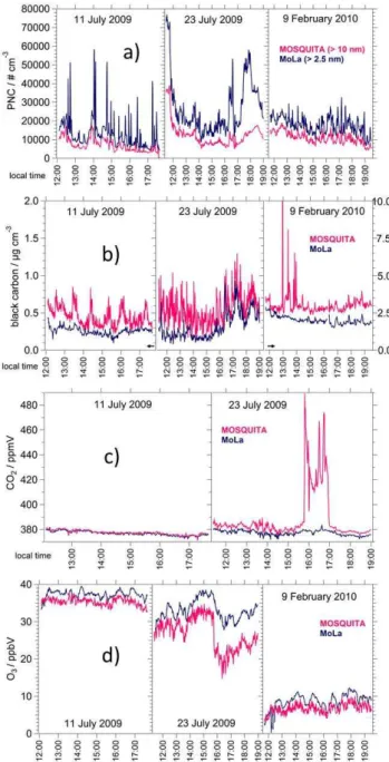
Particle number concentration: for the particle number concentration measurements we expect significant differ-ences because the lower size cut-off of the CPCs is different. Figure 1a shows the time series of the particle number con-centration recorded during the three intercomparison time periods by the CPCs in MoLa and MOSQUITA. While the MoLa-CPC has a lower cut-off of 2.5 nm the MOSQUITA-CPC detects particles larger than 10 nm and the MoLa in-strument yields always similar or larger number concentra-tions as the other instrument. Accounting for the different size ranges the agreement of total number and temporal vari-ations is satisfying and approximate comparability of the two measurements is given if no extreme concentrations of nucle-ation mode particles are present.
HR-ToF-AMS data sets the same data processing routines were applied (m/z calibration, baseline correction, instru-ment background measureinstru-ments and additional calibration parameters) different values for the collection efficiency are used during the summer campaign. For the MoLa data set a standard collection efficiency of 0.5 (Matthew et al., 2008) is applied during both campaigns. For the MOSQUITA data set the same value was used in winter; however, a value of 1.0 was applied for the summer data set. This unusual collection efficiency is justified on the one hand by long-term experi-ences with the MOSQUITA instrument, reflecting instrumen-tal features of this HR-ToF-AMS. On the other hand includ-ing all intercomparison measurements (not only AMS inter-comparisons, but also AMS comparison with additional PM1
measurements) carried out during both campaigns it seems to be appropriate to apply different collection efficiencies for the MOSQUITA summer and winter AMS data. A second difference between the data sets is the mode of operation of the two HR-ToF-AMSs. The MoLa instrument switched be-tween 10 s in the mass spectrum mode and 10 s in the particle time-of-flight mode, both in V-mode (medium resolution but high sensitivity) only. The MOSQUITA instrument applied shorter mode switching times, and also measured in V-mode only. During the summer campaign the AMS switched be-tween 3 s in mass spectrum mode and 2 s in particle time-of-flight mode. In winter it switched between 5 s in mass spec-trum mode and 5 s in particle time-of-flight mode. Due to the shorter measurement time a higher temporal resolution (but also larger uncertainty) of the AMS data were achieved com-pared to the MoLa instrument.
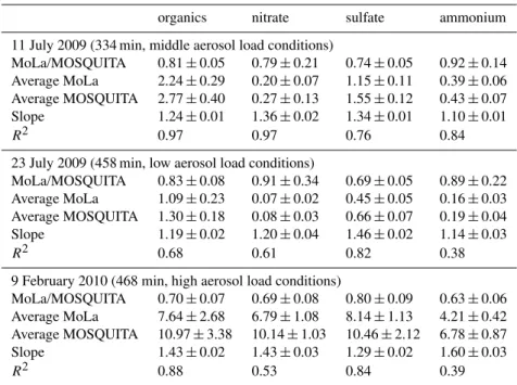
In Table 3 the correlation parameters (slope and re-gression coefficient R2) of linear fits of the MoLa versus MOSQUITA data for particulate organic, sulfate, nitrate and ammonium of the three intercomparison times are listed, as well as average ratios of mass concentrations of MoLa to MOSQUITA data and mean concentration values of both instruments. The given uncertainties represent the standard deviations of the respective parameters, which include am-bient variations as well as instrumental noise. It can be seen that the MOSQUITA AMS measured always higher species mass concentrations than the MoLa instrument. Dur-ing the summer campaign the average ratio of the MoLa to the MOSQUITA AMS concentrations is about 0.80; dur-ing the winter campaign this ratio seems to be lower with about 0.70. The R2 values are between 0.84 and 0.97 for the first intercomparison period, which implies that tempo-ral variations are observed by both instruments similarly. The lowR2values for nitrate and ammonium during the second intercomparison (summer) can be explained by low ambi-ent concambi-entrations of these componambi-ents near or below the detection limit of the MOSQUITA AMS. In winter ambi-ent concambi-entrations were well above the detection limits of both instruments; however, especially for ammonium theR2 value (0.39) is still low. Calibration errors of one or both instruments can be the reason for the observed differences
Fig. 1. Time series of the particle number concentration (PNC,
panel a), black carbon concentration (panel b), CO2 mixing ratio
(panel c) and O3mixing ratio (panel d) recorded during the
inter-comparison time periods on 11 July 2009, 23 July 2009 and 9 Febru-ary 2010 by the devices in MoLa (blue) and MOSQUITA (pink).
CO2data recorded by MOSQUITA are only available during the
summer intercomparisons.
similarly by both instruments during all three intercompari-son periods.
The overall uncertainty of AMS data is, including all un-certainties of operation mode, instrumental differences, dif-ferent inlet setups, calibrations and analysis variations, about 30 % (Canagaratna et al., 2007), so the observed differences are within the range of uncertainty. Similar ranges of un-certainty were experienced during other intercomparison ex-ercises as well (Bahreini et al., 2009). Intercomparisons of the MoLa and the MOSQUITA aerosol mass spectrometers with AMS instruments at the stationary measurement sites show similar discrepancies (Freutel et al., 2013; Crippa et al., 2013).
Black carbon mass concentration: Fig. 1b shows the time series of the black carbon concentration recorded during the three intercomparison time periods by the MAAP devices in MoLa and MOSQUITA. Although black carbon mass con-centrations were measured with two identical instruments during the summer campaign the MOSQUITA device mea-sured on average about 40 % more than the MoLa device. In winter the difference was slightly lower at about 30 %. Long-term temporal variations were similarly represented by both instruments, but the concentrations measured by the MOSQUITA device seem to be much noisier. This significant difference in absolute concentrations can only be explained by calibration errors, deterioration of instrumental compo-nents and/or differences in the inlet systems. The MoLa MAAP sampled the aerosol through a PM1 cyclone (only
particles up to 1 µm were measured) while the MOSQUITA device was not operated in combination with a specific size selective aerosol inlet. Comparison results of the MoLa in-strument with black carbon measurements at the stationary sites can be found in Freutel et al. (2013). In this publication the difference of identical MAAP instruments is satisfyingly small at about 10 %.
CO2mixing ratio: Fig. 1c shows the time series of the CO2
mixing ratios recorded during the summer intercomparison time periods by the CO2devices in MoLa and MOSQUITA.
During the winter intercomparison the MOSQUITA device was not operational. During the first summer intercompari-son (11 July 2009) both instruments show very good agree-ment of the recorded CO2mixing ratios and the differences
in absolute concentrations were below 1 %. The second sum-mer intercomparison (23 July 2009) reveals larger differ-ences of the recorded CO2 mixing rations. Between 16:00
and 17:00 local time the MOSQUITA instrument measured a strong CO2concentration enhancement of about 50 ppmV.
Since no external reason could be found for this (e.g. a strong local CO2emission near the MOSQUITA inlet), an internal
measurement device error is assumed.
O3 mixing ratio: Fig. 1d shows the time series of the
O3mixing ratios measured during the three intercomparison
time periods by the O3 devices in MoLa and MOSQUITA.
O3mixing ratios also show comparable temporal variations.
On average the MoLa instrument measured about 5 % more
than the MOSQUITA device during the first summer inter-comparison and 25 % more during the second one. In win-ter the difference is about 30 %. The MoLa instrument is less sensitive than the one in MOSQUITA and the difference could be explained by different instrument designs and cal-ibration errors. Additional intercomparisons of both instru-ments to O3 devices at the fixed measurement sites show
very good agreement for the MoLa instrument (summer and winter) and good comparability for the MOSQUITA device (only validated for summer, because in winter no additional intercomparison data are available).
NOx mixing ratio: due to calibration issues of the
MOSQUITA instrument in summer an intercomparison can only be done for the winter data. Here the MOSQUITA in-strument measured 30 % less than the MoLa device. This dis-crepancy can be caused by calibration errors of one or both devices. The MoLa instrument applies a molybdenum con-verter for the NOx measurements, which causes additional
uncertainty of the measured NOxmixing ratios (Steinbacher
et al., 2007). Intercomparisons of the MoLa device with in-struments at the fixed measurement sites show good results in summer and winter. No additional intercomparison data are available for the MOSQUITA device in winter.
In summary, the agreement of most parameters, except black carbon and NOx, is within the range of uncertainty
of the instruments and the data are sufficiently accurate for combined analysis. Aerosol sampling artifacts occurring in the two inlet systems and small scale (few metres) aerosol concentration differences should not have influenced the in-tercomparison in a significant way.
2.3 Data preparation for analysis
Mobile measurements can be adversely influenced by ad-ditional factors that are often negligible during stationary measurements. Especially local contamination caused by, for example, vehicles driving in front of the mobile laboratory or emission sources near the street is problematic for the processing of the measurement data. Pollution from these sources can dominate the measured data, since typically the concentrations of local emissions are large compared to am-bient values. Those contaminations have to be removed from the data set when ambient air is supposed to be measured, e.g. when background and plume emissions are investigated. Sep-arately analysed, the data points associated with local pol-lution contain valuable information about, for example, on-road pollutant emission indices or pollutant emission fluxes from point sources like industrial plants.
Table 3.Average ratios of MoLa data to MOSQUITA data, average concentration values in µg m−3of both HR-ToF-AMS instruments and
two correlation parameters∗(slope and regression coefficientR2) for the three intercomparison time intervals for the measured variables
sub-micron particulate organics, nitrate, sulfate and ammonium. Chloride data are not listed, because ambient values were below the detection limit most of the time. The given uncertainties represent one standard deviation.
organics nitrate sulfate ammonium
11 July 2009 (334 min, middle aerosol load conditions)
MoLa/MOSQUITA 0.81±0.05 0.79±0.21 0.74±0.05 0.92±0.14
Average MoLa 2.24±0.29 0.20±0.07 1.15±0.11 0.39±0.06
Average MOSQUITA 2.77±0.40 0.27±0.13 1.55±0.12 0.43±0.07
Slope 1.24±0.01 1.36±0.02 1.34±0.01 1.10±0.01
R2 0.97 0.97 0.76 0.84
23 July 2009 (458 min, low aerosol load conditions)
MoLa/MOSQUITA 0.83±0.08 0.91±0.34 0.69±0.05 0.89±0.22
Average MoLa 1.09±0.23 0.07±0.02 0.45±0.05 0.16±0.03
Average MOSQUITA 1.30±0.18 0.08±0.03 0.66±0.07 0.19±0.04
Slope 1.19±0.02 1.20±0.04 1.46±0.02 1.14±0.03
R2 0.68 0.61 0.82 0.38
9 February 2010 (468 min, high aerosol load conditions)
MoLa/MOSQUITA 0.70±0.07 0.69±0.08 0.80±0.09 0.63±0.06
Average MoLa 7.64±2.68 6.79±1.08 8.14±1.13 4.21±0.42
Average MOSQUITA 10.97±3.38 10.14±1.03 10.46±2.12 6.78±0.87
Slope 1.43±0.02 1.43±0.03 1.29±0.02 1.60±0.03
R2 0.88 0.53 0.84 0.39
∗Linear fit through zero for MOSQUITA AMS data versus MoLa AMS data (15 min averages of organics,
nitrate, sulfate and ammonium, respectively).
measurement data were corrected for the residence time in the inlet system. Due to the optimisation and characterisa-tion of both inlet systems particle losses during transport to the instruments are known and of a negligible order of mag-nitude. For more details see Bukowiecki et al. (2002), Mohr et al. (2011) and Drewnick et al. (2012).
To obtain as much information as possible especially from HR-ToF-AMS data several advanced analysis methods are available. Two of them, PMF and PIKA were used for the processing of this data set and are introduced in Sects. 2.3.2 and 2.3.3.
2.3.1 Removal of local contamination
Several methods, like automatic concentration peak removal, were tested to obtain uncontaminated mobile data sets that are not influenced by local pollution emissions and the “video tape analysis procedure” finally was selected. More details on different local pollution removal strategies and examples of “before – after” time series are presented in Drewnick et al. (2012).
Video tape analysis procedure: during the analysis of the MEGAPOLI data set it has become apparent that the most consistent method to identify local contamination is to anal-yse the video tapes of mobile measurements recorded by the webcam in the driver’s cabin. Therefore several criteria for contaminated time periods were defined:
– Times whilst driving through a village/town due to higher traffic, heating, cooking and other human ac-tivities.
– Times when a vehicle is less than about 150 m in front of the mobile laboratory or when there is significant traffic on the road including the opposite lane.
– Times while the driving velocity of the mobile labora-tory is low increasing the possibility of contamination by the own exhaust.
– Times while next to the street a source of local con-tamination is visible, for example a burning fire or a working tractor.
– Times while driving through a tunnel, because exhaust emissions might be accumulated.
time consuming method (approximately 30 min of analysis time for 60 min of measurement time). Meanwhile, there has been some effort made to automate the local pollution detec-tion. During mobile MoLa measurements, it is now possible to note via a mouse click the time period and the kind of pol-lution event occurring. With this information a contamination mask is created, which can be used to analyse the data.
Only for a first interpretation of the individual measure-ment trips the contaminated data sets can be used to avoid the time-consuming pollution removal procedure for data sets that are not used for later analysis. For all further analysis of the Paris emission plume only the uncontaminated data were used to obtain best results and conclusions.
2.3.2 Positive matrix factorization
Positive matrix factorization (PMF) is used to identify aerosol types in the atmosphere that can be associated with different sources. The underlying statistical procedure is based on the principle of mass conservation. Such methods, which use measured ambient concentrations as inputs and es-timate source contributions, are generally known as receptor models. They are used to reduce large data sets by estima-tion of number of potential aerosol sources and composiestima-tion of aerosols related to them (“factors” that explain the data variability). Part of this study is to identify different sources of organic aerosol contributing to the emission plume from the Paris agglomeration. The importance of organic aerosol is demonstrated by its high fraction of the total submicron aerosol mass. It can consist of multiple organic components and the scientific interest in formation and transformation processes in the atmosphere is high (Jimenez et al., 2009; Lanz et al., 2010). Therefore, PMF became one of the stan-dard analysis techniques for HR-ToF-AMS data in the past few years (Zhang et al., 2011). With this method it is pos-sible to extract factors representing not only organic aerosol of different sources but also organic aerosol of different ox-idation states which is correlated to the age of the aerosol. However, the mathematical algorithm of PMF has several un-certainties by itself (e.g. start value “seed” of the calculation and rotational freedom of the solution given by the parameter “fpeak”) and the freedom of the user inputs and interpretation adds additional uncertainty. Comparison of PMF results with external time series of other instruments and with mass spec-tra from known sources are tools for embedding those results in a greater context to identify the potential chemical nature of a certain PMF factor. For more details about the under-lying mathematical algorithm and the applied software, we refer to Paatero and Tapper (1994), Paatero (1997), Lanz et al. (2007) and Ulbrich et al. (2009).
PMF of MEGAPOLI mobile data sets: PMF was applied to both mobile unit mass resolution AMS data sets includ-ing all data sampled durinclud-ing the respective measurement cam-paigns. For the MoLa summer data set the organic aerosol can be described by five factors (hydrocarbon-like organic
aerosol (HOA), low-volatile oxygenated organic aerosol (LV-OOA), cooking-related organic aerosol (COA) and two types of oxygenated organic aerosol with higher volatility). In win-ter the 6 factor solution (HOA, LV-OOA, COA, two types of organic aerosol associated with biomass burning and one fac-tor with higher volatility) provides a good approximation of the composition of the particulate organic matter. PMF for the MOSQUITA mobile data sets resulted in mainly two fac-tors for the summer (HOA and LV-OOA) and an additional third factor for the winter campaign which is also associated with biomass burning. HOA and LV-OOA are especially in-teresting for the identification of the Paris emission plume. HOA is mainly associated with fresh emissions (Zhang et al., 2005), e.g. from traffic like in the emission plume air masses, while LV-OOA mainly represents highly oxidized long-range transported air masses which characterise the ambient back-ground atmosphere. In Sect. 3.3 an example of the MoLa PMF results is presented. For further description of the men-tioned factors (HOA, LV-OOA, etc.), we refer to Zhang et al. (2011). Details about the extracted factors and their identi-fication using correlations with external time series and mass spectra, quantified uncertainties and interpretation of the sci-entific content of the PMF results would exceed the scope of this overview paper. There will be further publications based on these mobile data sets including a detailed PMF discus-sion (e.g. von der Weiden-Reinmüller et al., 2013).
2.3.3 Peak integration by key analysis
PIKA (Peak Integration by Key Analysis; ToF-AMS Anal-ysis Software Homepage, 2013) is another advanced analy-sis software tool for the speciation and quantification of HR-ToF-AMS data. PIKA is based on SQUIRREL (SeQUential Igor data RetRiEvaL; ToF-AMS Analysis Software Home-page, 2013), the standard software for basic analysis of AMS data, e.g. for application of calibration parameters and to ob-tain chemically resolved mass concentration time series or particle size distributions. In newer versions PIKA includes APES (Analytical Procedure for Elemental Separation; ToF-AMS Analysis Software Homepage, 2013), a software tool for the separation of high resolution AMS signals into their elemental components. In this study PIKA was mainly ap-plied for the retrieval of the O/C ratio of the organic aerosol which is a marker for the oxidation state and therewith the age of the aerosol. In Sect. 3.2 an example of aerosol with low O/C ratio as marker for fresh emissions in the Paris plume is presented. More details about PIKA, SQUIRREL and APES can be found on the developers’ website (ToF-AMS Analysis Software Homepage, 2013).
2.4 Measurement strategies
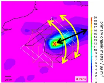
Fig. 2.Prev’Air Paris emission plume actual day forecast for 31 Jan-uary 2010 18:00:00 UTC during the winter field campaign. The colour code indicates the concentration of primary organic matter, a marker for fresh air pollution. Paris is located in the middle of the straight black and grey lines (concentration colour code: yel-low/orange, red X), which indicate potential flight routes for the re-search aircraft. The yellow arrows demonstrate cross-section mea-surements of several ten to hundred kilometres at two different dis-tances to Paris. The black arrow indicates axial measurements start-ing at the outer areas of Paris up to about 200 km away from the city.
measurement is most useful for a specific day regional plume prediction maps for pollutant markers like primary organic matter were provided by Prev’Air (Honoré et al., 2008).
Prev’Air plume prediction maps: the Prev’Air forecast system (Prev’Air, 2013) started in 2003 and is based on global, European and national forecast simulations. The aim is to provide daily air quality forecast and re-analysis maps of pollutant markers like O3, NO2, PM10and PM2.5for
Eu-rope and France. Air quality maps are provided as 2-day (e.g. simulating on Monday the air quality situation occurring on Wednesday), 1-day and actual day forecasts and as retrospec-tive re-analysis. These re-analysis maps – a combination of a posteriori simulations and observations – are the most objec-tive representation of the pollution situation. They were also used for our mobile measurements analysis (e.g. to check which part of the measurement route was located within the Paris emission plume). For the campaign planning specific forecasts were made available by INERIS (Institut National de l‘Environnement Industriel et des Risques, Verneuil en Halatte, France), running the Prev’Air system with an en-hanced forecast frequency (3 h) and additional compounds (e.g. primary and secondary organic matter, see Fig. 2).
Measurement planning: for the measurement planning 1-day forecast maps were applied for a rough route planning on the evening before the measurement day. A combination of high resolution printed fold-up maps and actual day forecast
maps was used in the morning of the measurement day to decide on the actual driving route. Ideal routes for the inves-tigation of a megacity emission plume avoid forests, streets with heavy traffic, larger villages and towns and regions with strong local pollution like proximate industrial plants. In gen-eral, mobile measurements were carried out on minor roads with less traffic to avoid local pollution sources as much as possible. Stationary measurement sites were chosen applying similar considerations. Additional attention was paid to pro-vide a free undisturbed flow of the air masses to the sampling location. So, places behind trees or in valleys were avoided as well as places downwind of local pollution sources like villages or major streets.
In summary, MoLa performed a total of 31 mobile (in-cluding 6 axial trips) and 25 stationary measurements of sev-eral hours measurement time each during both campaigns. MOSQUITA measured 17 times on the road, including one mobile measurement late in the evening. Stationary measure-ments were performed with MOSQUITA only for intercom-parison purposes.
2.4.1 Cross-section measurements
To distinguish between ambient background and emission plume influenced aerosol and trace gas loadings of the ground-level atmosphere cross-section measurements are beneficial. A cross-section measurement usually starts in a region not influenced by the emission plume, then crosses the plume at a nearly constant distance to the city and ends again in background air masses. Several cross-section mea-surements at different distances from the city provide addi-tional information about dilution and aging processes in the plume during transport. Applying this type of measurement, it is also possible to investigate the cross-sectional structure of the plume and dilution processes at the plume border. If the predicted emission plume was distinct and reasonably sta-ble in direction over a sufficient number of hours (to finish a significant fraction of the measurement during this time), cross-section measurements were carried out. Problems with this type of measurement occur when the plume is changing its direction during the day. To cover the plume as well as background air masses usually takes several hours. So a shift-ing plume can appear deformed in the measured data with a broader, narrower or more heterogeneous shape than it was in reality.
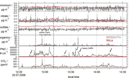
Fig. 3.Temporal behaviour of aerosol parameters primarily associated with long-range transported pollution (ammonium, nitrate and sulfate) and variables reflecting mainly locally and regionally produced pollution (organics, particle number concentration (PNC, > 2.5 nm for MoLa
and > 10 nm for MOSQUITA) and CO2). The red lines represent the MoLa stationary measurement data and the grey lines the MOSQUITA
mobile measurement data. The two vertical dashed lines frame the mobile measurement range within the city area of Paris; the arrows indicate measurement times with heavy traffic on the street. The time series were measured by MOSQUITA (outward trip) and MoLa during the summer campaign on 20 July 2009. The time resolution of the data is 1–7 s (MOSQUITA) and 1–60 s (MoLa). The stationary measurement location of MoLa and the mobile measurement track (outward trip) of MOSQUITA are marked in the map of Fig. 4.
2.4.2 Axial measurements
To get insight into the spatial extent of the plume, i.e. up to which distance from the city it can be observed as sig-nificantly above background level, axial measurements are beneficial. The quasi-Lagrangian character (following an in-dividual air parcel along its trajectory) of such measurements also allows investigating atmospheric conversion processes, like oxidation of organic aerosol or ozone build-up from pre-cursor gases, during transport and dilution with increasing distance to Paris. In Fig. 2 the black arrow represents ax-ial measurements starting at the outer suburbs of Paris and reaching as far as about 200 km away from the city. For this type of measurement a distinct emission plume with constant wind conditions is necessary. A wind shift of a few degrees over several hours is tolerable and the axial measurement route still should be located inside the plume. The megacity Paris is an area source of pollution and therefore the emission plume can be expected to have a width of more than ten kilo-metres. Appropriate weather conditions were identified only during three days during both campaigns. An additional is-sue with this type of measurement appears when major roads or larger towns are located in the predicted plume direction. Fresh pollution from these local sources will mix with the Paris emission plume and change its physical and chemical properties like average oxidation state of the organic aerosol or number concentration of small particles.
MoLa carried out three axial trips up to 180 km away from the city border during the summer campaign. In winter three axial trips up to 100 km distance from Paris were performed. MOSQUITA performed most of the mobile measurements as a combination of cross sections and axial trips to cover a wide area. With this strategy it is easier to measure the emis-sion plume even if the plume direction is slightly uncertain or changing. The disadvantage of this method is that the dis-tance to Paris that can be covered within several hours is not as large as on a straight axial trip. In Sect. 3.3 a measure-ment example of an axial trip performed during the summer campaign by MoLa is presented.
2.4.3 Stationary measurements
This type of measurement was often chosen when plume predictions were not sufficiently stable for mobile measure-ments. Measurement sites downwind of Paris allow measur-ing the emission plume for several hours at a certain distance and locations upwind of Paris were used for ambient back-ground measurements.
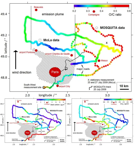
Fig. 4.Combined results of MoLa (line of squares) and MOSQUITA (dotted line) mobile applications of four cross-section measurements through the Paris emission plume during the summer campaign on 29 July 2009. Both data sets have a time resolution of 1 min, but were smoothed for this graph (boxcar smoothing algorithm, 10 points). The regional wind direction was constantly from South on this day (black
arrow). The track is colour-coded by the O/C ratio (upper large graph), black carbon mass concentration (lower left graph) and CO2mixing
ratio (lower right graph). The urban area of Paris is marked by the big red dot, the Paris metropolitan area is indicated by the grey shaded area. The cross (“X”) marks the location of the stationary measurements on 20 and 27 July 2009 (see Sects. 3.1 and 3.4). The black thin line shows the track of the MOSQUITA mobile measurement on 20 July 2009 (see Sect. 3.1).
(Beekmann et al., 2014; Freutel et al., 2013). A few mea-surements show both, the Paris emission plume and the at-mospheric background values when the wind direction was shifting. For these data sets the investigation of plume struc-ture and homogeneity is possible. An example of such a mea-surement is presented in Sect. 3.4. For meamea-surements located in the direction of the predicted plume and in line with sta-tionary measurement sites (connected flow between all mea-surement locations) investigation of conversion and dilution processes during transport is also possible. This approach was adopted by Freutel et al. (2013) for the MEGAPOLI campaigns.
3 Examples for the different measurement strategies
In this section four measurement examples are presented to demonstrate the successful application of the developed mea-surement strategies and analysis methods for the investiga-tion of the Paris emission plume.
3.1 Long-range transport of pollution versus local and regional pollution
direction of Paris. This mobile measurement (for the track see Fig. 4) included passes through the city centre of Paris (a large and inhomogeneous source of fresh pollution) on the outward and return journey from the starting point (fixed suburb measurement site in the South-West of Paris). At the same time MoLa performed a stationary measurement at about 30 km distance to the border of the metropolitan area also in the North-East of Paris (for measurement location also see Fig. 4). The Paris emission plume was advected to the North-East direction, so both mobile laboratories should have encountered air masses influenced by Paris.
In Fig. 3 time series of six aerosol and gas phase variables measured by MOSQUITA during the outward trip can be seen. Additionally, the same measurement variables recorded by the stationary MoLa are shown. Three time series repre-sent aerosol species that are associated with long-range trans-ported pollution (ammonium, nitrate, sulfate) and the other three are dominated by local and regional pollution (organ-ics, particle number concentration, CO2). For better
illustra-tion of the different temporal and spatial behaviour of fresh and aged pollution markers no local pollution removal proce-dure (as described in Sect. 2.3.1) was applied to the presented data.
The time series of particulate organic matter shows signatures of both pollution types. The measured organ-ics are a mixture of long-range transported highly oxi-dized (aged) organic aerosol, semi-volatile medium-aged or-ganic aerosol, primarily produced hydrocarbon-like oror-ganic aerosol (mainly associated with traffic emissions) and freshly produced organic aerosol caused by various emission sources (e.g. cooking, biomass burning). In Fig. 3 the fresh and local fractions of the organic aerosol can be clearly identified by the various concentration peaks. The long-range transported part of the organic aerosol is represented by an underlying slowly varying concentration level of about 1 to 2 µg m−3, also measured by the stationary MoLa.
The time series of the particle number concentration (> 10 nm for MOSQUITA) is also dominated by frequent concentration changes due to the various sources probed dur-ing the drive. The long-range transported fraction (accumu-lated and grown particles with a mode diameter larger than 100 nm) of the particle number concentration is small com-pared to the large number of freshly emitted small particles with a few nanometers particle diameter.
Concerning CO2, Fig. 3 shows mainly the peak
concen-trations from fresh pollution, due to the axis scaling. Af-ter several hours of transportation the fresh CO2
contribu-tions are totally diluted in the surrounding air masses, but momentary CO2 concentrations measured near the source
can reach about twice the global background concentrations which can be seen in the presented time series measured by MOSQUITA. CO2 mixing ratios measured by MoLa show
nearly constant values around 378 ppmV (±2 ppmV), be-cause no nearby local emission sources influenced the mea-surement location. A similar temporal behaviour can be seen
for particle number and organic aerosol mass concentrations during this MoLa stationary measurement.
In contrast to the behaviour of the pollutants related to fresh emissions the time series of particulate ammonium, nitrate and sulfate measured with both mobile laboratories show only small and slow variations in time despite rapid fluctuations around the actual background value, mainly caused by instrumental noise (especially for ammonium, where the measured values are close to the detection limit of this species for the MOSQUITA AMS). This is a typical behaviour for substances that change only on large temporal and spatial scales under the influence of different air masses. Of course, in reality there are not only the two extremes of very local fresh pollution plumes and completely homoge-neously distributed long-range transported air masses. There are also air masses where secondary aerosol is inhomoge-neously mixed because the precursor substances have been emitted inhomogeneously.
3.2 Cross section through the Paris emission plume:
combination of MoLa and MOSQUITA data
Measurement example: on 29 July 2009 the Paris emission plume was constantly advected towards the North. Both mo-bile laboratories carried out two cross-section measurements each in the North and North-East region around Paris. MoLa performed two cross sections at 10 km and 30 km distance from the Paris metropolitan area and MOSQUITA two cross-sectional transects at 20 km and 40 km distance. In Fig. 4 the measurement tracks of both mobile laboratories colour-coded with the O/C ratio, the black carbon mass concentra-tion and the CO2mixing ratio are presented on a map of the
region. Low O/C ratios indicate less oxidized fresh organic aerosol, high O/C ratios indicate highly oxidized aged or-ganic aerosol (Aiken et al., 2007, 2008). The low O/C ratio values (< 0.2) in the South and East of Paris are caused by heavy traffic on major roads and thus local contamination. The interesting result of this measurement is the low values measured in the North of Paris – carried out on minor roads with less traffic – which are clearly associated with the Paris emission plume. At the same distance to the city but in the North-East direction much higher O/C ratios (> 0.6) were ob-served indicating aged background air masses not influenced by the city. Simultaneously with low O/C values increased black carbon and CO2 concentrations were observed,
con-firming the identification of the emission plume in the North of Paris.
long-range transported pollution was probed on this day. This detailed picture of plume and background air masses in a wide area around Paris can be obtained due to the combi-nation of the data from both mobile laboratories.
The emission plume as visible in the O/C ratios (and also black carbon and CO2concentrations) in Fig. 4 looks rather
homogeneous with a definite structure (i.e. the lowest O/C ratios in the centre of the plume, with gradually increasing ratios to both sides) even in the nearest cross section per-formed by MoLa only 20 km away from the border of Paris. Within this distance one could expect a more inhomogeneous structure due to the short transportation time of about 1 h (av-eraged wind speed about 20 km h−1 on this day) from this large diversified emission source. For more details on this and about the plume structure analysis we refer to the future publication by von der Weiden-Reinmüller et al. (2013).
3.3 Axial measurement: exploring the spatial extent of the emission plume
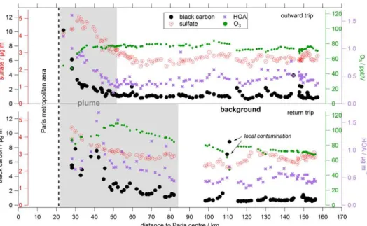
Measurement example: on 1 July 2009 weather conditions and the predicted plume were sufficiently stable and well-defined for an axial measurement. The North-Eastern wind advected the Paris emission plume to the South-West, where MoLa performed an axial trip up to 160 km from Paris cen-tre. On this day only MoLa was deployed. Figure 5 presents black carbon, HOA and sulfate mass concentrations and O3
mixing ratios versus the distance to the centre of Paris. In the upper part of the graph results from the outward trip carried out during the morning can be seen, in the lower part results from the return trip during the afternoon are shown. Although the contamination removal was applied to the data, still few locally influenced high concentration values can be seen.
Nevertheless, a clear decrease of black carbon and HOA concentrations in the emission plume can be observed with increasing distance to Paris. On the outward trip the emis-sion plume that is observable with our measurements extends approximately up to 30 km distance from the outer areas of Paris which is equal to 50 km distance to Paris centre. Dur-ing the day the emission plume seems to develop and inten-sify. On the return trip the range of the detected plume in-creased to a distance of about 80 to 100 km from Paris cen-tre. The decrease in concentration with increasing distance from the city is mainly caused by dilution of the emission plume in surrounding background air masses. The wind di-rection was nearly constant during the measurement, so we assume that we measured constantly in the lateral plume core and the decrease in fresh pollutants should not be caused by leaving the plume. We expect within this time frame of sev-eral hours no significant black carbon sinks like dry deposi-tion and there was no precipitadeposi-tion causing wet deposideposi-tion on this day. Moreover, HOA is not transformed into secondary organic aerosol within this time frame. In regions near the city black carbon concentrations are approximately ten times higher (7 to 10 µg m−3) than in background air masses (0.5
to 1 µg m−3). HOA concentrations vary from 1.5 µg m−3near
the city to around 0.5 µg m−3in background air masses.
During the return trip at a distance of about 110 km to Paris centre concentration peaks of black carbon (> 6 µg m−3) were measured, although local contamination was removed by video analysis. In this region two larger villages with a commercial area are located resulting in a regionally higher traffic volume and therefore causing a regional pollution hot spot. Here the limits of the applied local pollution removal procedure become obvious, because only “visible” (in the video tapes) contamination sources in front of the vehicle can be identified. Measurements on a near bypass road (where no local pollution source is recorded by the webcam) can still be affected by locally distributed emissions. Neverthe-less, the spatial extent of the Paris emissions plume can be clearly seen and also quantified in the presented data. The described decreasing concentrations with increasing distance from Paris were not only observed in black carbon and HOA mass concentrations, but also in related fresh pollution mark-ers like PAH and CO2(not shown in Fig. 5).
Additionally, we calculated the average HOA to BC ra-tio for plume and background air masses for both axial trips. If both substances are only diluted in the advected emission plume and no conversion processes occur, this ratio should not change with increasing distance to Paris. For both trips the HOA to BC ratio is on average about 0.3 inside the plume, while in background air masses the ratio is higher: 0.4 for the outward trip and 0.6 for the return trip. This could be ex-plained by higher HOA than BC background levels compared to the respective pollutant burden in the emission plume. Pos-sibly, HOA emitters are more frequently distributed also in rural areas than BC emitters. It was not possible to iden-tify transformation processes due to the HOA to BC ratio with increasing distance to Paris and results on transforma-tion processes in the advected emission plume will be dis-cussed in a separate publication (von der Weiden-Reinmüller et al., 2013).
O3mixing ratios are decreased by about 30 ppbV near the
city and reach a nearly constant background value of about 80 ppbV at a distance of approximately 30 km from the city border. The ozone depletion near the city is caused by in-creased NO concentrations from fresh emissions in the city. During the outward trip (before noon) the atmospheric con-ditions seem to have not been suitable for significant ozone production downwind of Paris. In contrast to this, on the return trip (in the afternoon) we observe ozone production from precursor gases emitted in Paris at a distance of about 30 km away from the city border. Here the O3 mixing
ra-tios peak around 110 ppbV. Lower O3concentrations are also
observed near the city (around 10 km from the city border); background O3levels of 70 to 80 ppbV are reached at a
Fig. 5.Black carbon (large black dots), HOA (purple stars) and sulfate (red dots and crosses) mass concentrations and O3mixing ratio (small
green dots) versus distance to Paris centre measured during an axial trip on 1 July 2009 by the mobile laboratory MoLa. In the upper part of this graph results of the outward trip carried out during the morning are presented, in the lower part results from the return trip during the afternoon. The data points identified as significantly influenced by the Paris emission plume are indicated by the grey area. The time resolution of the data is 1 min.
Surprisingly, during this axial trip also long-range trans-ported secondary pollution markers like sulfate (see Fig. 5) and nitrate show a decrease in concentration (a factor of two to three for sulfate and a factor of four to ten for nitrate) with increasing distance to Paris. It is possible that long-range transported pollution was mixed with the probed megacity emissions. At the downtown and suburb South-West mea-surement sites an increase in sulfate was observed during the morning of 1 July 2009, followed by decreasing concen-trations in the afternoon and enhanced values again in the evening. In contrast to this, fresh pollutant markers showed a different temporal behaviour on this day. However, dur-ing other axial trips like the one performed with MoLa on 25 July 2009 increased concentrations of sulfate are not mea-sured near Paris but at a distance of about 100 km. These are both indicators that we measured the Paris emission plume with some mixed-in long-range transported pollution.
Another explanation for the observed decrease in concen-tration of most of the measured pollutants with increasing distance to Paris could be that the few axial trips carried out had been performed mainly during the same time of day (starting in the morning in Paris and returning in the evening). Usually, the atmospheric boundary layer develops during the day and breaks down in the evening. High mea-sured concentrations could therefore also be correlated to a low boundary layer height, accidentally associated with mea-surements near the city. However, the measured data of the axial trip on 25 July 2009 show a contrary trend for some of the measured variables: no enhancement of ammonium and
sulfate could be observed during the morning and evening hours near the city, but around noon at a distance of more than 100 km away from Paris the concentrations are approx-imately two times higher. So we assume that the boundary layer influence is small at least for secondary and large scale transported pollutants. The boundary layer influence on pri-mary and locally emitted pollution is however difficult to as-sess during these types of measurements.
3.4 Stationary measurements: plume crossing
during wind shift
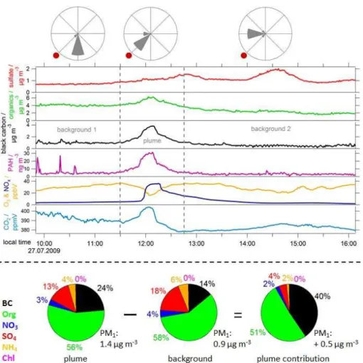
Fig. 6.CO2(light blue), O3(yellow) and NOx(dark blue) mixing ratios as well as PAH (purple), black carbon (black), particulate organics
(green) and sulfate (red) mass concentrations measured during a stationary measurement on 27 July 2009 by MoLa. The measurement location (centre of windrose plots) was in the North-East of Paris (red dot in windrose plots) situated about 30 km from the city border. The wind was shifting from South to West during the measurement as indicated by the wind rose plots. The grey vertical dashed lines frame the time period when the Paris emission plume was sampled. The time resolution of the data is 1 min. However, internal averaging settings
of the NOxmodule caused longer averaging times (several minutes, slightly varying with concentration changes) during this stationary
measurement for this instrument. Additionally, the average PM1aerosol mass concentrations and compositions for plume and background air
masses are provided in the lower part of this figure. The total PM1mass concentration was calculated as the sum of BC (MAAP instrument),
Org, NO3, SO4, NH4and Chl (AMS instrument) concentrations. The subtraction of the average background concentration from the average
plume concentration gives the plume contribution to total PM1.
and the emission plume was sampled during the time be-tween the grey dashed lines in Fig. 6.
In Fig. 6 time series of O3, NOxand CO2mixing ratios as
well as black carbon, PAH, particulate organics and sulfate mass concentrations are presented for this scenario. There is a clear enhancement in CO2, NOx, black carbon,
organ-ics and PAH concentrations around noon caused by the Paris emissions. The concentrations increase about sevenfold com-pared to background values measured on this day for black carbon, about tenfold for PAH and about twelvefold for NOx.
The CO2concentration is increased by about 25 ppmV
com-pared to the lowest values measured on this day by MoLa between 12:30 and 13:00 local time. O3 shows a reduced
mixing ratio from a maximum of 37 ppbV to a minimum
of 16 ppbV due to high NOxconcentrations associated with
fresh emissions in the Paris area.
In contrast, sulfate concentrations show no significant en-hancement during this time. SO2(not presented in this graph)
shows a minor increase during this time period, but has ob-viously not yet been transformed into sulfate until the ar-rival of the air masses at the measurement site. A clear en-hancement in particulate sulfate can be seen in the afternoon around 14:30 local time on this day. This seems to be long-range transported pollution (e.g. from industrial plants emit-ting SO2at larger distance to the measurement site), because
no simultaneous enhancement can be seen in black carbon or PAH concentrations. CO2 and O3 show slightly higher