Early-Holocene warming in Beringia and its mediation by sea-level and vegetation changes

(1)

CPD

11, 873–932, 2015

Early-Holocene warming in Beringia

P. J. Bartlein et al.

Title Page

Abstract Introduction

Conclusions References

Tables Figures

◭ ◮

Back Close

Full Screen / Esc

Printer-friendly Version Interactive Discussion

Discussion

P

a

per

|

Discussion

P

a

per

|

Discussion

P

a

per

|

Discussion

P

a

per

|

Clim. Past Discuss., 11, 873–932, 2015 www.clim-past-discuss.net/11/873/2015/ doi:10.5194/cpd-11-873-2015

This discussion paper is/has been under review for the journal Climate of the Past (CP). Please refer to the corresponding final paper in CP if available.

Early-Holocene warming in Beringia and

its mediation by sea-level and vegetation

changes

P. J. Bartlein1, M. E. Edwards2,3, S. W. Hostetler4, S. L. Shafer4, P. M. Anderson5,

L. B. Brubaker6, and A. V. Lozhkin7

1

Department of Geography, University of Oregon, Eugene, Oregon, USA

2

Geography and Environment, University of Southampton, Southampton, UK

3

Alaska Quaternary Center, University of Alaska, Fairbanks, Alaska, USA

4

U. S. Geological Survey, Corvallis, Oregon, USA

5

Quaternary Research Center, University of Washington, Seattle, Washington, USA

6

School of Environmental and Forest Sciences, University of Washington, Seattle, Washington, USA

7

Northeast Interdisciplinary Research Institute, Far East Branch Russian Academy of Sciences, Magadan, Russia

Received: 13 February 2015 – Accepted: 17 February 2015 – Published: 30 March 2015

Correspondence to: P. J. Bartlein ([email protected])

(2)

CPD

11, 873–932, 2015

Title Page

Tables Figures

◭ ◮

Back Close

Full Screen / Esc

Discussion

P

a

per

|

Discussion

P

a

per

|

Discussion

P

a

per

|

Discussion

P

a

per

|

Abstract

Arctic land-cover changes (e.g., expansion of woody vegetation into tundra and effects of permafrost degradation) that have been induced by recent global climate change are expected to generate further feedbacks to the climate system. Past changes can be used to assess our understanding of feedback mechanisms through a combination

5

of process modelling and paleo-observations. The sub-continental region of Beringia (Northeast Siberia, Alaska, and northwestern Canada) was largely ice-free at the peak of deglacial warming and experienced both major vegetation change and loss of per-mafrost when many arctic regions were still ice covered. The evolution of Beringian climate at this time was largely driven by global features, such as the amplified

sea-10

sonal cycle of Northern Hemisphere insolation and changes in global ice volume and atmospheric composition, but changes in regional land-surface controls, such as the widespread development of thaw lakes, the replacement of tundra by deciduous forest or woodland, and the flooding of the Bering–Chukchi land bridge, were probably also important. We examined the sensitivity of Beringia’s early Holocene climate to these

15

regional-scale controls using a regional climate model (RegCM). Lateral and oceanic boundary conditions were provided by global climate simulations conducted using the GENESIS V2.01 atmospheric general circulation model (AGCM) with a mixed-layer ocean. We carried out two present day simulations of regional climate, one with mod-ern and one with 11 ka geography, plus another simulation for 6 ka. In addition, we

20

performed five ∼11 ka climate simulations, each driven by the same global AGCM boundary conditions: (i) 11 ka “Control”, which represents conditions just prior to the major transitions (exposed land bridge, no thaw lakes or wetlands, widespread tundra vegetation), (ii) sea-level rise, which employed present day continental outlines, (iii) vegetation change, with deciduous needleleaf and deciduous broadleaf boreal

vege-25

(3)

CPD

11, 873–932, 2015

Title Page

Tables Figures

◭ ◮

Back Close

Full Screen / Esc

Discussion

P

a

per

|

Discussion

P

a

per

|

Discussion

P

a

per

|

Discussion

P

a

per

|

regional-scale controls strongly mediate the climate responses to changes in the large-scale controls, amplifying them in some cases, damping them in others, and, overall, generating considerable spatial heterogeneity in the simulated climate changes. The change from tundra to deciduous woodland produces additional widespread warming in spring and early summer over that induced by the 11 ka insolation regime alone and

5

lakes and wetlands produce modest and localized cooling in summer and warming in winter. The greatest effect is the flooding of the land bridge and shelves, which pro-duces generally cooler conditions in summer but warmer conditions in winter, and is most clearly manifest on the flooded shelves and in eastern Beringia. By 6 ka continued amplification of the seasonal cycle of insolation and loss of the Laurentide ice sheet

10

produce temperatures similar to or higher than those at 11 ka plus a longer growing season.

1 Introduction

For the northern high latitudes, climate models simulate significant regional-scale changes that are consistent with presently observed changes in global climate (ACIA,

15

2004, p. 146; Serreze et al., 2007) and with projected future global climate changes (e.g., Collins et al., 2013). The distribution and physiological status of vegetation, com-bined with other features of the terrestrial surface, significantly influence energy, water, and carbon exchange between the land and the atmosphere (e.g., Bonan et al., 1995; Chase et al., 1996; Chapin et al., 2005). Such exchanges produce feedback to local,

20

regional, and global climates, which, in turn, a_ffect plant distribution and physiology (e.g., Thomas and Rowntree, 1992; Foley et al., 1994). Thus the potential exists for land-cover status to enhance or mitigate climatic change through either positive or negative feedbacks to energy, water, and carbon budgets (Oechel et al., 1993; Lynch et al., 1999; Chapin et al., 2005) and to generate significant feedbacks to the seasonal

25

(4)

CPD

11, 873–932, 2015

Title Page

Tables Figures

◭ ◮

Back Close

Full Screen / Esc

Discussion

P

a

per

|

Discussion

P

a

per

|

Discussion

P

a

per

|

Discussion

P

a

per

|

Large areas of the arctic and sub-arctic land surface are underlain by continuous or discontinuous permafrost that affects soil and drainage properties. At the landscape scale, land cover is a complex mosaic of tundra (tall shrub, mesic tussock, dry heath, fellfield and barrens, etc.), forest (evergreen conifer, deciduous conifer, and succes-sional hardwoods), wetlands, surface standing water and lakes, and glaciers. Northern

5

ecosystems have received considerable attention in the global budgets of carbon diox-ide and methane, because soils, peatlands, and lakes are important sources and sinks of these gases and highly sensitive to changes in surface energy exchange (Oechel et al., 1993; Bonan et al., 1995; Zimov et al., 2006; Walter et al., 2006; Walter An-thony et al., 2014). Climatically induced changes in vegetation distribution, especially

10

those involving replacement of tundra by forest, and changes in soil and permafrost properties will have a dramatic impact on these processes (Smith and Shugart, 1993; Smith et al., 2005). Further, biophysical land-atmosphere coupling via albedo, interac-tions between vegetation and snow, and modulation of sensible and latent heat fluxes have important climatic implications on seasonal-to-decadal time scales (Harvey, 1988;

15

Thomas and Rowntree, 1992; Bonan et al., 1995; Sturm et al., 2005; Myers-Smith et al., 2011).

Currently observed changes linked to 20th-century warming in the Arctic and sub-Arctic include the expansion of large shrubs in northern Alaskan and Siberian tundra (Sturm et al., 2001, 2005; Forbes et al., 2010), negative trends in evergreen tree growth

20

(Barber et al., 2000; McGuire et al., 2010), and rapidly thawing permafrost (Osterkamp and Romanovsky, 1999; Romanovsky et al., 2010). Vegetation competition-succession model simulations suggest the potential for more extreme shifts from evergreen for-est to woody-deciduous and/or treeless biomes as a transient response to warming (Chapin and Starfield, 1997). Ultimately these changes and the land-surface

interac-25

(5)

CPD

11, 873–932, 2015

Title Page

Tables Figures

◭ ◮

Back Close

Full Screen / Esc

Discussion

P

a

per

|

Discussion

P

a

per

|

Discussion

P

a

per

|

Discussion

P

a

per

|

with observed land-cover changes and thus assess climate-model sensitivity to such changes. Unglaciated regions of the Arctic warmed early in the Holocene (Kaufman et al., 2004) and experienced considerable terrestrial change over a few millennia; we use this period to conduct a series of sensitivity experiments with a regional climate model driven by a general circulation model (GCM) simulation for 11 ka.

5

Beringia (Northeast Siberia, Alaska, and northwestern Canada) is well-suited for such an exercise because a diverse range of paleoenvironmental records is available over the interval from 21 000 yr ago to present (21 to 0 ka BP). The early Holocene (ca. 12 to 10 ka BP) was a time of major climate warming, and paleoenvironmetal data doc-ument shifts among tundra, woody-deciduous and woody-evergreen dominance

(Ed-10

wards et al., 2005). We designed and conducted a series of regional climate-model simulations based on observed changes in vegetation, substrate, and sea level in Beringia during the period of major warming centered on the onset of the Holocene (ca. 11 ka BP). Our primary goal is to assess the sensitivity of the simulated climates to regional land-atmosphere interactions and feedbacks ca. 11 ka. We also simulated

15

6 ka conditions, which were climatically more stable but still warmer than present.

1.1 Study area

The regional climate-model domain (Fig. 1) is larger than the region typically defined as Beringia (Hopkins, 1982); it encompasses the Indigirka drainage eastward to Chukotka and Kamchatka in the western portion of the study domain, and Alaska, a

consider-20

able portion of northwest Canada and the adjacent seas in the eastern portion of the study domain. The regional topography is complex, including several mountain ranges, plateaus, low-lying tectonic basins and flat coastal plains. The easternmost parts of the study area lay under the Laurentide ice sheet during the last glaciation; other ar-eas were a_ffected only by local mountain glaciation (Kaufman et al., 2004; Elias and

25

Brigham-Grette, 2007).

(6)

CPD

11, 873–932, 2015

Title Page

Tables Figures

◭ ◮

Back Close

Full Screen / Esc

Discussion

P

a

per

|

Discussion

P

a

per

|

Discussion

P

a

per

|

Discussion

P

a

per

|

climate is influenced by the status of a mid-tropospheric trough-ridge system. An upper-level trough is centered on average to the east of China, and northward of the trough ra-diational cooling generates a strong surface high over Siberia. Consequent northwest-erly winds block the incursion of maritime air into easternmost Asia and are linked to January temperatures as low as−40◦C (Mock et al., 1998). High pressure over

north-5

west Canada is associated with cold January temperatures of about−30◦C. Conditions are somewhat warmer (−15◦C) along the southern coast of Alaska (Mock et al., 1998; Edwards et al., 2001). Summer temperature is driven by high radiation receipts and the advection of warm air into both eastern and western portions of the study area via sub-tropical high pressure systems that develop to the south. Summer temperatures range

10

from ∼5–15◦C across the study area (Steinhauser, 1979; World Meteorological Or-ganization, 1981). Temperatures generally increase from north to south, except where there is local coastal cooling, and in interior basins of Alaska, which can experience July temperatures of 15◦_{C or higher. In eastern Asia cooler temperatures inland relate}

to northerly flow due to the position of the East Asian trough over eastern Siberia.

15

Precipitation is low in winter; inland January total precipitation long-term means may be<25 mm (Steinhauser, 1979; World Meteorological Organization, 1981), but south-ern regions of the study area receive abundant orographically enhanced precipitation of a meter per year or more. Typically, there is a late summer precipitation maximum related to mid-latitude cyclones that are steered across the region by the East Asian

20

trough. July precipitation ranges from 50–100 mm; in eastern Asia precipitation levels increase southwards, while Alaskan interior basins are generally drier than western or coastal areas.

At a larger scale, the tendency for frequent cyclogenesis over Eurasia, Alaska, and Canada in summer is associated with the development of an Arctic frontal zone. The

25

(7)

CPD

11, 873–932, 2015

Title Page

Tables Figures

◭ ◮

Back Close

Full Screen / Esc

Discussion

P

a

per

|

Discussion

P

a

per

|

Discussion

P

a

per

|

Discussion

P

a

per

|

changes in climate, the forest-tundra border may exert a stabilizing effect on regional climate as the relatively high-albedo tundra side of the border will remain cooler than the lower-albedo forest side of the border (Ritchie and Hare, 1971; TEMPO Members, 1996; Lynch et al., 2001). In contrast, when large, externally driven changes in regional climate occur, shifts in the location of the forest-tundra border may locally amplify the

5

climatic change (Foley et al., 1994).

On a regional scale, the distribution of precipitation is strongly influenced by topog-raphy, particularly in coastal Alaska and Canada, but also in upland regions in the in-terior (e.g., the Brooks Range), where precipitation is greater than in lowland regions. The same is true in western Beringia, where precipitation is enhanced in the Chersky,

10

Kolyma, Koryak, and Verkhoyansk mountain ranges and in coastal mountains in the Kamchatka Peninsula.

Land-surface properties also influence local precipitation. For example, the summer precipitation maximum in the Mackenzie Basin is associated with a minimum in large-scale vapor-flux convergence (Walsh et al., 1994), suggesting that substantial summer

15

precipitation is derived from within-basin recycling of water vapor via evapotranspiration from the tundra and boreal forest. The numerous Alaskan lakes have a strong e_ffect on surface fluxes and heat storage (Oncley et al., 1997; Rivers and Lynch, 2004), and it is possible that widespread fields of lakes that characterize some parts of the region may be an important source of feedback at the regional level (Subin et al., 2012).

20

Modern vegetation is a mosaic of forest and tundra communities. The northern Siberian coastlands, western and northern Alaska, Banks Island and the Canadian Beaufort Sea coastlands are characterized by tundra. Shrubs of varying stature dom-inate in many areas, but grasses and sedges characterize wet coastal zones. Alpine tundra occurs above boreal forest treeline at altitudes over 500–800 m. Forests in the

25

Asian portion of the study region are dominated by the deciduous coniferLarix gmelinii

(larch). River valleys also support gallery forests ofPopulus suaveolens (poplar) and

(8)

CPD

11, 873–932, 2015

Title Page

Tables Figures

◭ ◮

Back Close

Full Screen / Esc

Discussion

P

a

per

|

Discussion

P

a

per

|

Discussion

P

a

per

|

Discussion

P

a

per

|

in Northeast Siberia and is a common understory component of larch forests. The ever-green conifers,Picea glaucaandP. mariana(white and black spruce) dominate forests in Alaska and northern Canada; here, hardwoods such as Populus tremuloides and

P. balsamifera(aspen, balsam poplar) andBetula neoalaskana andB. papyrifera (pa-per birch) form seral stands after disturbances such as fire. Permafrost is continuous

5

in the north and discontinuous to the south of the region (Rekacewicz, 1998). Exten-sive wetlands occur across the region related to topography and permafrost-impeded drainage. The southeastern part of the study area includes grassland and shrubland of the Columbia Plateau and interior Canada.

1.2 Key changes in land-cover features during deglacial warming

10

At the last glacial maximum (LGM: 25–18 ka BP) global sea level was lowered by ∼120–135 m (Fairbanks, 1989; Yokoyama et al., 2000). The shelves of the Bering and Chukchi Seas and Arctic Ocean were exposed, and Alaska and Siberia formed a con-tinuous land mass. The Laurentide and Cordilleran ice sheets (LIS, CIS) lay to the east and southeast of Beringia, and mountain glaciations occurred in the Brooks, Chersky,

15

Kolyma, Koryak, and Verkhoyansk mountain ranges and other upland regions. Con-siderable eolian deposition occurred in lowland areas, particularly the northern coastal plain of Siberia, the Anadyr lowlands, and interior basins and the northern coastal plains of Alaska and Canada (Hopkins, 1982).

By 11 ka BP, rapidly melting continental ice sheets (and the large-scale atmospheric

20

circulation changes associated with them), rising sea level, and increasing summer in-solation generated a series of terrestrial changes in Beringia (Kaufman et al., 2004). Sea level rose rapidly during deglaciation (Fairbanks, 1989); estimates suggest the Bering Strait formed about 11 ka BP, but several millennia passed before the remaining expanses of exposed continental shelf were completely inundated (Manley, 2002;

Keig-25

(9)

CPD

11, 873–932, 2015

Title Page

Tables Figures

◭ ◮

Back Close

Full Screen / Esc

Discussion

P

a

per

|

Discussion

P

a

per

|

Discussion

P

a

per

|

Discussion

P

a

per

|

Williams and Yeend, 1979; Burn, 1997; Romanovskii et al., 2000; Walter et al., 2007). This period also marked the inception of wetlands and peat growth, which developed further in subsequent millennia (Jones and Yu, 2010). Thaw-lake formation accelerated in the early Holocene after 11 ka BP, but decreased subsequently (Walter et al., 2007; Walter Anthony et al., 2014). It is likely that the current proportion of land occupied by

5

lakes (for example 5–40 % on the Arctic Coastal Plain) was attained during the early Holocene (Walter et al., 2007).

Over the period from ca. 15–8 ka BP, a sequence of changes in zonal vegetation occurred in Beringia. Across the region, graminoid-forb tundra that typified the LGM was replaced around 15–14 ka BP bySalix- andBetula-dominated shrub tundra,

gen-10

erally interpreted to be initially of low stature (Anderson et al., 2004; Edwards et al., 2005). Over the next few millennia much of the region became dominated by woody taxa, although the species composition differed between the Asian and North American sectors. Between ca. 13–10 ka BP, lower-elevation regions of unglaciated Alaska and Canada saw the expansion of deciduous tall-shrub and woodland vegetation; in Asia

15

at this time vegetation cover at lower elevations included deciduous shrubs, hardwood trees such asBetula platyphylla (Asian birch) withLarix in the western portion of the region (Edwards et al., 2005). Between ca. 11–10 ka BP evergreen conifer forest de-veloped in the eastern sector. The evergreenPinus pumilaspread across the western sector, within and beyond theLarixforest limits. Shrub tundra remained dominant north

20

of treeline across the whole region, except in the far north, where dwarf-shrub or herb-dominated tundra occurred. These general vegetation features persist to the present day, although there have been subtle changes in tree limits and forest composition (Anderson et al., 2004).

We focused on three features of 11 ka land-cover change for our model experiments:

25

(10)

CPD

11, 873–932, 2015

Title Page

Tables Figures

◭ ◮

Back Close

Full Screen / Esc

Discussion

P

a

per

|

Discussion

P

a

per

|

Discussion

P

a

per

|

Discussion

P

a

per

|

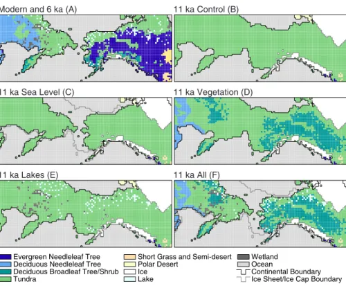
terrain. We additionally examined the output from a simulation for 6 ka, a time when insolation patterns were still markedly different from present (Fig. 2) but land cover and continental outlines were similar to present.

2 Methods

2.1 Climate models

5

We used a hierarchical modeling procedure that involves running an atmospheric gen-eral circulation model (AGCM) to simulate global climate and provide continuous (every 6 h) time series of sea-surface temperature (SST), sea ice, and lateral boundary con-ditions (vertical profiles of temperature, wind, humidity) for the regional climate model (RCM) simulations. In previous studies, this hierarchy of models has been

demon-10

strated to reproduce present day climate and simulate regional-scale responses to changes in the large-scale controls that compare favourably with reconstructions of those responses from paleoenvironmental data (Hostetler and Bartlein, 1999; Hostetler et al., 1994, 2000). This method of coupling GCMs with RCMs to downscale climate is now widely used in climate assessments (e.g., Mearns et al., 2012).

15

The AGCM is version 2.01 of the GENESIS climate model (Thompson and Pollard, 1995). Version 2.01 and later versions of GENESIS have been used extensively for paleoclimate simulations (Pollard and Thompson, 1997; Joussaume et al., 1999; Pinot et al., 1999; Ruddiman et al., 2005; Tabor et al., 2014; Alder and Hostetler, 2014). The atmospheric component of GENESIS is coupled with the Land Surface eXchange

20

model, LSX (Thompson and Pollard, 1995), to simulate surface processes and to ac-count for the exchange of energy, mass and momentum between the land surface and the atmospheric boundary layer. We used model resolutions of T31 (∼3.7◦ in latitude and longitude) and 2◦

×2◦ in latitude and longitude for the atmosphere and surface, respectively. The model was run using a coupled mixed layer ocean (50 m in depth),

25

(11)

CPD

11, 873–932, 2015

Title Page

Tables Figures

◭ ◮

Back Close

Full Screen / Esc

Discussion

P

a

per

|

Discussion

P

a

per

|

Discussion

P

a

per

|

Discussion

P

a

per

|

a number of sensitivity experiments in which we varied sea-ice parameters to optimize the simulation of present day sea ice. The boundary conditions for the RegCM simula-tions span the last 10 yr of 65 yr long GENESIS simulasimula-tions.

The RCM is version two of the RegCM regional climate model (RegCM2; Giorgi et al., 1993a, b). Newer versions of RegCM now exist that offer more options and

im-5

proved computational performance (Pal et al., 2007), but the atmospheric core of the model has remained essentially the same as RegCM2. Our version of RegCM2 is cou-pled with the LSX surface-physics package used in GENESIS. We employed a model grid-resolution of 60 km (roughly 0.5◦_{) for the simulations (Fig. 1a and b). To optimize}

our sensitivity tests we modified RegCM2 to include orbitally determined insolation,

10

a lake model (Hostetler and Bartlein, 1990) to simulate lake temperature and ice and their feedbacks with the boundary layer, and we modified aerodynamic (e.g., rough-ness height) and biophysical (e.g., leaf area index) vegetation parameters in LSX to be consistent with the properties of the reconstructed Beringia vegetation. For the lake sensitivity tests, we represented the spatial distribution of shallow thaw lakes by

spec-15

ifying time-appropriate (i.e., 0, 6 and 11 ka) model grid points as water. For all lakes, we specified a depth of 4 m and moderately high turbidity, which is su_fficient to real-istically capture the seasonal cycle of lake-atmosphere feedbacks in our experiments. The vegetation and lake implementations are discussed in more detail below. Each RegCM2 simulation was run for 10 yr and the first 2 yr are excluded from our analysis

20

to allow soil-moisture fields to equilibrate. Ten-year simulations with 8 yr averages are sufficient to allow for model spin up and to isolate mean climate responses associated with our array of prescribed changes in paleogeography, which, in most cases, repre-sent substantial perturbations between and among experiments. In contrast to GCMs where time-slice simulations may take 10s to 100s of years to reach equilibrium, RCM

25

(12)

CPD

11, 873–932, 2015

Title Page

Tables Figures

◭ ◮

Back Close

Full Screen / Esc

Discussion

P

a

per

|

Discussion

P

a

per

|

Discussion

P

a

per

|

Discussion

P

a

per

|

2.2 Experimental design

We designed our experiments to isolate and quantify the potential controls of the early Holocene climate of Beringia. Our experiments thus include a set of varied atmospheric boundary conditions and surface changes that we describe and summarize below.

2.2.1 Present-day, 6 ka and 11 ka boundary conditions

5

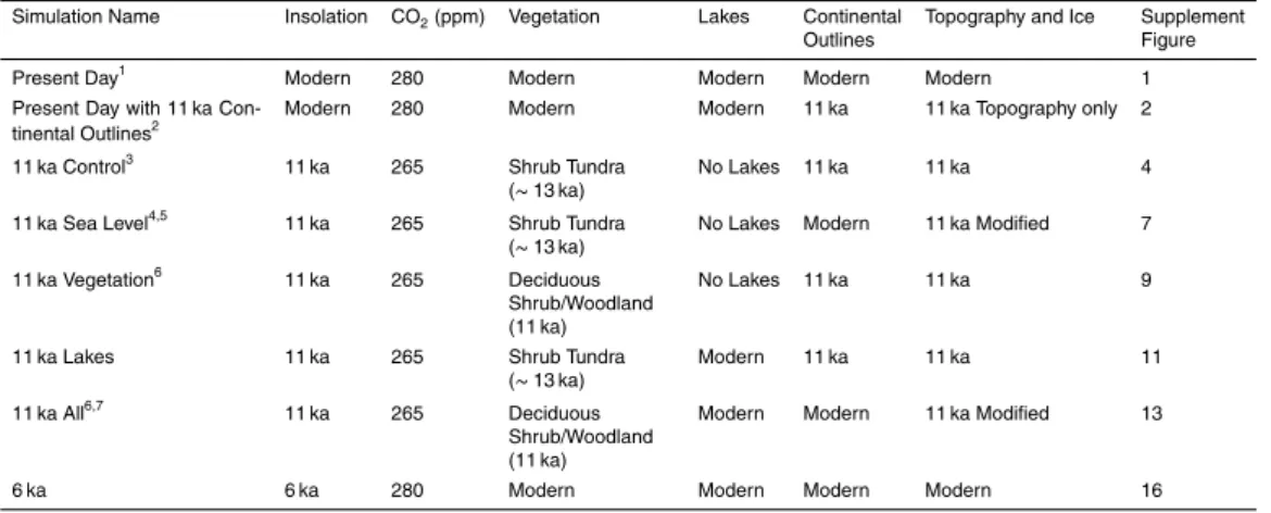
The AGCM and RCM each require the specification of insolation, surface boundary conditions (including 11 ka continental outlines and land-surface and ice-sheet topog-raphy), atmospheric greenhouse gas composition, land-cover (vegetation and soils), and lake and wetland distribution (Table 1). Insolation for present, 6 ka and 11 ka was specified following Berger (1978) (Fig. 2). Atmospheric composition (e.g., CO2) was set

10

to pre-industrial values (i.e., 280 ppm) for the Present-Day and 6 ka simulations, and to 265 ppm (Monnin et al., 2001) for the 11 ka simulations.

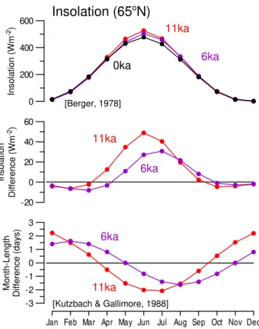
The impact of the variations in the obliquity (tilt) and climatic-precession (time-of-year of perihelion) elements of the Earth’s orbit can be seen in the anomalies of insolation and the lengths of the different months and seasons (Berger, 1978; Kutzbach and

15

Gallimore, 1988; Fig. 2). At 11 ka, perihelion was in late June, the tilt of the Earth’s axis was 24.2◦_{, and the eccentricity was about 0.019 (as compared to the present values}

of early January, 23.4◦_{, and 0.017). Consequently, June insolation was about 50 W m}−2

greater than present at 65◦_{N. However, owing to its elliptical orbit, the Earth moves}

faster near the time of perihelion (Kepler’s law of equal areas), and at 11 ka June and

20

July were about 2.0 days shorter than present (assuming a 360-day year and 30-day months; Kutzbach and Gallimore, 1988). At 6 ka, perihelion was in September, the tilt was 24.1◦_{, and eccentricity was about the same as at 11 ka. The maximum insolation}

anomaly consequently occurred later, in July, and was about 30 W m−2 _{greater than}

present at 65◦_{N. Owing to the later time of year of perihelion at 6 ka than at 11 ka,}

25

(13)

CPD

11, 873–932, 2015

Title Page

Tables Figures

◭ ◮

Back Close

Full Screen / Esc

Discussion

P

a

per

|

Discussion

P

a

per

|

Discussion

P

a

per

|

Discussion

P

a

per

|

11 and 6 ka were similar. Overall, the early-Holocene boreal summer and the mid-Holocene late summer could be described as shorter and “hotter” than at present.

Figure 1 shows the 0 ka (present) and 11 ka topography, ice and continental outlines, respectively. Ice-sheet elevations for the 11 ka AGCM simulation were derived from Peltier (1994), and for the 11 ka RCM simulations from Hostetler et al. (2000).

Land-5

surface elevations (and hence the continental outlines), were specified for each model at 11 ka by interpolating Peltier (1994) ICE-4G topographic anomalies (i.e., 11 ka minus 0 ka differences) and applying these to the present day grid point elevation in the model. In the RCM at 11 ka, this procedure yields a land mask with an extensive land bridge between North America and Asia (Fig. 1b). We constructed a second set of land

ele-10

vations to depict the flooded land bridge by superimposing the present day land mask over the 11 ka elevations, and setting all values outside of the present day shoreline mask to sea level (0.0 m; Fig. 1a). Because the topography in the region consists of either broad coastal plains with low slopes or rather steep terrain in coastal mountain regions, we did not need to “taper” the coastal elevations when creating this elevation

15

data set.

Land-cover characteristics were expressed in both models as Dorman–Sellers “biome” types (Dorman and Sellers, 1989), which implicitly include the specification of soil characteristics associated with the vegetation. For the AGCM simulation these biomes closely followed Lynch et al. (2003). For the RCM simulations, present day

land-20

cover characteristics (including wetlands) were derived from the Global Land Cover Characteristics data base (http://edc2.usgs.gov/glcc/globdoc2_0.php). The spatial pat-tern of the land-cover types was simplified to create general patpat-terns at the same spatial resolution of information available from paleorecords for describing the 11 ka land-cover type patterns, including wetlands (Figs. 3 and 4). We further specified the

25

(14)

CPD

11, 873–932, 2015

Title Page

Tables Figures

◭ ◮

Back Close

Full Screen / Esc

Discussion

P

a

per

|

Discussion

P

a

per

|

Discussion

P

a

per

|

Discussion

P

a

per

|

vegetation-type parameter values in LSX (e.g., leaf-area index, canopy structure and height, etc.).

2.2.2 Present-day, 6 ka and 11 ka surface characteristics

Surface characteristics describing land cover, sea level and the distribution of lakes and wetlands were defined for the present day, 6 ka and 11 ka RCM simulations. For

5

the 11 ka RCM simulations, we used five separate sets of surface characteristics (land mask, topography, and land-cover type) that are described in detail below. The first set represents conditions prior to 11 ka, and represents the “point of departure” for the 11 ka experiments (and hence is referred to here as the “11 ka Control”). A sec-ond set represents csec-onditions after the 11 ka changes (referred to here as “11 ka All”).

10

Three other sets were defined to examine the individual effects of land-bridge flooding (“11 ka Sea Level”), vegetation change from tundra to deciduous tall shrub/woodland (“11 ka Vegetation”), and thaw-lake/wetland development (“11 ka Lakes”; Fig. 4b–f; Ta-ble 1). In each case, paleoenvironmental data indicate that full development of the sea level, vegetation, and thaw-lake/wetland changes took centuries to millennia, the

ma-15

rine transgression being the most long-lived. However, as our study features an equi-librium sensitivity experiment, we created just two steady-states of 11 ka land cover, representing conditions close to the onset of changes (11 ka Control) and conditions when all the changes were fully expressed (11 ka All). We also defined two sets of sur-face characteristics for the present day, in order to separate the effects of land bridge

20

flooding from the other boundary-condition changes.

2.2.3 Present-Day simulation

The Present-Day (0 ka) simulation land cover included modern vegetation (Fig. 4a) defined as a mosaic of tundra and needleleaf forest (as described in Sect. 1.1), with short grass and semi-desert vegetation in the extreme southeast of the study area. The

25

(15)

CPD

11, 873–932, 2015

Title Page

Tables Figures

◭ ◮

Back Close

Full Screen / Esc

Discussion

P

a

per

|

Discussion

P

a

per

|

Discussion

P

a

per

|

Discussion

P

a

per

|

continental outlines, which created a land mask with the modern Bering Strait between Asia and North America.

2.2.4 Present-day simulation with an 11 ka land mask

We defined a second set of present day boundary conditions by combining the modern land-cover data with an 11 ka land mask including elevation data. This set of boundary

5

conditions is used to separate the simple effects of the land-bridge flooding from the combined effects of all of the other “paleo” boundary conditions.

2.2.5 6 ka simulation

We also used modern land cover (Fig. 4a) for the 6 ka simulation. Lakes and wet-lands were well established at 6 ka (Walter et al., 2007; Jones and Yu, 2010).

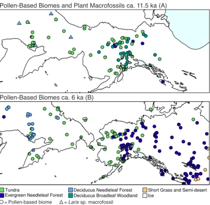
Pollen-10

based biomes for 6 ka defined by the BIOME 6000 project (Prentice et al., 2000; Ed-wards et al., 2000a; Bigelow et al., 2003) were used as a guide to vegetation cover. In Siberia, the modern land cover (Fig. 4a) closely approximates the 6 ka biome dis-tribution (Fig. 3b), while in eastern Beringia the western evergreen needleleaf forest limit is displaced eastwards. Almost all post-glacial sea-level rise had occurred by 6 ka

15

(Manley, 2002) and the continental outlines are only slightly different from modern (as shown in Fig. 3b); we considered the vegetation and coastline differences not signifi-cant enough to require a separate 6 ka land cover mask.

2.2.6 11 ka Control simulation

The late-glacial development of Beringian vegetation proceeded over several millennia

20

from herbaceous vegetation, through low shrubs to tall shrubs and deciduous wood-land (see Sect. 1.2). We use the low-shrub tundra to represent the vegetation for the 11 ka Control simulation; its surface properties differ little from the preceding herba-ceous tundra vegetation (not modelled here). We also included the 11 ka LIS, CIS, and mountain glaciers and ice caps, but not lakes and wetlands (Fig. 4b). Topography

(16)

CPD

11, 873–932, 2015

Title Page

Tables Figures

◭ ◮

Back Close

Full Screen / Esc

Discussion

P

a

per

|

Discussion

P

a

per

|

Discussion

P

a

per

|

Discussion

P

a

per

|

was defined using Peltier (1994) 11 ka geography, and by adding the paleo topographic anomalies to the present day elevations. The resultant RCM land mask features lower sea level, with the Bering land bridge in place between Asia and North America (see Sect. 2.2.1), and 11 ka land and ice topography.

2.2.7 Sea-Level simulation

5

The Sea-Level simulation was identical to the 11 ka Control simulation, but with topog-raphy defined using Peltier (1994) 11 ka geogtopog-raphy and modern sea level (Fig. 4b and c; see Sect. 2.2.1). This combination created an RCM land mask with 11 ka topogra-phy but a flooded land bridge (i.e., the modern Bering Strait) between Asia and North America.

10

2.2.8 Vegetation simulation

The 11 ka Vegetation simulation was identical to the 11 ka Control simulation with the exception of vegetation (Fig. 4d). To describe the changed vegetation for this simulation we used an approach involving several steps: the “biomization” of pollen data (Pren-tice and Webb, 1998; Bigelow et al., 2003), evidence from plant macrofossils (Edwards

15

et al., 2005; Binney et al., 2009) and expert knowledge. The latter was needed be-cause the biomized pollen maps and macrofossil records (Fig. 3) indicate broad trends in vegetation cover but hold too few data points to allow for quantitative spatial in-terpolation. We used records from the PARCS (Paleoenvironmental Arctic Sciences) database (http://www.ncdc.noaa.gov/paleo/parcs/index.html) falling nearest to 11.5 ka

20

in age to guide the placement of deciduous broadleaf woodland for the 11 ka Vege-tation simulation. This time slice gave the strongest signal of deciduous woodland in eastern Beringia, defining the deciduous broadleaf woodland biome at about half the sites across the region. Deciduous needleleaf (Larix) forest is not identified in far north-east Siberia at 11 ka by biomized pollen maps, likely due to lowLarixpollen counts in

25

(17)

CPD

11, 873–932, 2015

Title Page

Tables Figures

◭ ◮

Back Close

Full Screen / Esc

Discussion

P

a

per

|

Discussion

P

a

per

|

Discussion

P

a

per

|

Discussion

P

a

per

|

deciduous needleleaf forest at this time. However, the macrofossil record indicates the presence of deciduous broadleaf trees in east and west Beringia and ofLarixin Siberia (Edwards et al., 2005; Binney et al., 2009; Fig. 3). Based on these data, in east Beringia we specified 11 ka vegetation as a mosaic of low-stature shrub tundra and deciduous tall shrub/woodland, with the latter occupying lower elevations. In west Beringia we

5

specified 11 ka vegetation as a mosaic of low-stature shrub tundra and mixed decid-uous woodland, also determined by elevation. We designated the exposed shelf and land-bridge as low-stature shrub tundra, as in the 11 ka Control simulation, as little is known about past vegetation of the submerged land areas at ca. 11 ka; pollen and macrofossil data from sub-marine sediment cores taken from the Bering Sea suggest

10

shrub tundra (e.g., Elias et al., 1997; Ager and Phillips, 2008; Lozhkin et al., 2011).

2.2.9 Lakes simulation

The 11 ka Lakes simulation was identical to the 11 ka Control simulation with the ex-ception of lake and wetland cover. For the 11 ka Control simulation, no lakes or wet-lands were present on the RCM land cover grid. For the 11 ka Lakes simulation, lakes

15

and wetlands were represented by their modern distributions, placing lakes in regions where thaw lakes dominate the modern landscape (Fig. 4e). Lake and wetland distri-butions are derived from the Global Land Cover Characteristics data base described above. Thaw lakes probably extended onto Arctic Ocean shelves (Hill and Solomon, 1999; Romanovskii et al., 2000) that are now inundated, and they probably also formed

20

on the land bridge, but, as there is no information on their areal extent, we omitted lakes from these areas. The estimated average percent cover of lakes in modern lake-dominated landscapes from topographic maps and air photos is 5–40 %. In the exper-iment we used 40 % in order to provide the maximum possibility for a response in the simulation. Although thaw lakes are typically<1.0 to a few km in diameter, the

struc-25

(18)

CPD

11, 873–932, 2015

Title Page

Tables Figures

◭ ◮

Back Close

Full Screen / Esc

Discussion

P

a

per

|

Discussion

P

a

per

|

Discussion

P

a

per

|

Discussion

P

a

per

|

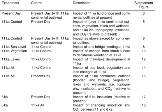
2.3 Summary

Our strategy was to examine a set of RCM simulations for 11 ka (Table 1) that together illustrate the impact of changes in vegetation, flooding of the land bridge, and develop-ment of thaw lakes and wetlands. We compared these 11 ka simulations with the 11 ka Control simulation and with simulations of the present day and 6 ka, to generate a set

5

of experiments (Table 2).

The simulations (described above; Table 1) can be summarized as:

1. Present Day, a simulation of the present day (0 ka) with realistic land cover (in-cluding vegetation, shorelines, and thaw-lake distribution). This is the control sim-ulation used to compare changes between 11 ka and present (Fig. 4a).

10

2. Present Day with 11 ka continental outlines, which used present climatology, veg-etation and lakes/wetlands but the 11 ka continental outlines (i.e., Fig. 4a but with continental outlines as in Fig. 4b). This simulation is used to partition the effect of changed sea level from that of other key drivers, such as insolation.

3. 11 ka Control, a simulation of conditions that prevailed prior to the changes in

15

vegetation, sea level, and thaw-lake distributions that are the focus of the study. This simulation functions as the control simulation against which the e_ffects of these land-cover changes at 11 ka are assessed (Fig. 4b).

4.–6. Three simulations: 11 ka Sea Level, 11 ka Vegetation, and 11 ka Lakes, which address each land-cover change in isolation (Fig. 4c–e).

20

7. 11 ka All, a simulation with all three land-cover changes (i.e., sea level, vegetation, lakes) included (Fig. 4f), to illustrate the combined effects of these controls.

8. 6 ka, a simulation using 6 ka boundary conditions and modern land cover (Fig. 4a), to explore a climate with modern boundary conditions, except for an amplified annual cycle of insolation.

(19)

CPD

11, 873–932, 2015

Title Page

Tables Figures

◭ ◮

Back Close

Full Screen / Esc

Discussion

P

a

per

|

Discussion

P

a

per

|

Discussion

P

a

per

|

Discussion

P

a

per

|

The experiments (Table 2) were as follows:

1. Present Day minus Present Day (with 11 ka continental outlines), which assesses the effect of the Bering Strait and modern coastline on modern climatology.

2. 11 ka Control minus Present Day, which describes the full change in conditions from 11 ka (before land-cover transformation) to modern conditions (including the

5

imposition of the Bering Strait).

3. 11 ka Control minus Present Day (with 11 ka continental outlines). This experi-ment reveals the e_ffect of insolation on the 11 ka climatology, as the large impact of sea-level change in the fully modern (Present Day) simulation is removed by using the 11 ka continental outlines.

10

4.–7. Three experiments to examine the one-at-a-time changes in sea level, vegetation, and thaw lakes and one experiment to examine the effect of all three of the above changes. The control in each case is 11 ka Control.

8. 11 ka All minus Present Day, which describes the full change in conditions from 11 ka (after land-cover transformation and including the imposition of the Bering

15

Strait) to modern conditions.

9. 6 ka minus Present Day, to examine the impact of mid-Holocene insolation anomalies.

10. 6 ka minus 11 ka All, to examine the climate change between 11 and 6 ka.

An experimental design that focuses on higher-order interactions among the controls

20

(20)

CPD

11, 873–932, 2015

Title Page

Tables Figures

◭ ◮

Back Close

Full Screen / Esc

Discussion

P

a

per

|

Discussion

P

a

per

|

Discussion

P

a

per

|

Discussion

P

a

per

|

3 Results

We present the modelling results in a series of figures that typically take the form of mapped monthly averages. Monthly averages are based on a 365-day year relative to the modern calendar (the e_ffects of the “calendar bias” (Sect. 2.2.1) are of continen-tal and hemispheric scale, and would not dominate the regional patterns of interest

5

here; Timm et al., 2008). In some cases the complete annual cycle is shown, in others summer and winter months (e.g., January and July) that highlight the more interesting patterns that emerge from the simulations. Maps representing results of specific simu-lations show 8 yr climatologies; those showing the results of experiments display diff er-ences between experimental and control simulation long-term means (i.e., anomalies).

10

Maps of all monthly values of key variables are available in the supporting online infor-mation (see Supplement).

3.1 Effect of the land-bridge flooding alone

The effect of the land-bridge flooding alone (i.e., with no other differences in boundary conditions between 11 ka and present) is assessed by the experiment that replaces

15

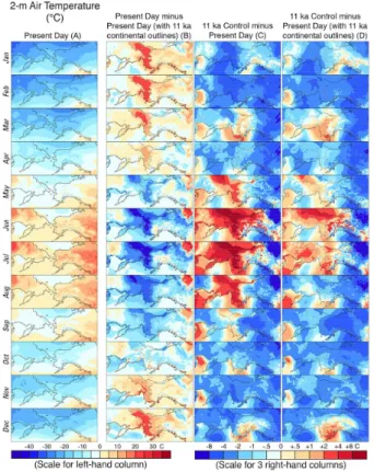
the modern land mask and elevation with one appropriate for 11 ka. For reference, Fig. 5a shows simulated modern monthly average air temperature for the study area. Figure 5b shows the impact on modern climate of “restoring” the 11 ka continental outlines (and topography). The anomalies shown are the long-term mean differences of the Present-Day simulation (Supplement Fig. 1) minus the Present-Day (with 11 ka

20

continental outlines) simulation (Supplement Fig. 2). The anomalies show the impact that flooding of the land bridge (and related topographical changes, like the collapse of the ice sheet) would have on the modern climate, if those paleogeographic changes occurred today (Supplement Fig. 3).

The prominent effect of shelf flooding is a reduction in the seasonality of 2 m air

tem-25

(21)

CPD

11, 873–932, 2015

Title Page

Tables Figures

◭ ◮

Back Close

Full Screen / Esc

Discussion

P

a

per

|

Discussion

P

a

per

|

Discussion

P

a

per

|

Discussion

P

a

per

|

with sea ice in the Present-Day simulation but which are land in the Present-Day (with 11 ka continental outlines) simulation (Fig. 5b). In the cool season (November through April) the temperature anomalies are strongly positive in the regions that are oceans in the Present-Day simulation but land in the Present-Day (with 11 ka continental outlines) simulation. (The impact of the decrease in elevation of the region that was ice-covered

5

at 11 ka is visible as a small area of positive summer temperature anomalies in the northeastern corner of the model domain.)

The genesis of these temperature anomalies lies in changes in the surface energy balance related to large differences in the heat capacity and albedo of land and water in the two present day simulations (Supplement Fig. 3b). Net shortwave radiation

anoma-10

lies are highly negative from May through August in the regions that change from land to ocean. This pattern shows the response to the large increase in albedo as dark land surfaces are replaced by ocean and permanent or seasonal sea ice. Positive net short-wave radiation anomalies occur over the region associated with the 11 ka ice sheet where elevation decreases. While present day land cover is used in both simulations,

15

the higher elevations in the Present-Day (with 11 ka continental outlines) simulation re-sults in a persistent snowpack in the northeastern part of the study area. Consequently, simulated net shortwave radiation is lower than present (thereby producing the positive anomalies). Net shortwave anomalies in the cool season (November through March) are close to zero, consistent with the low shortwave radiation inputs at that time of year.

20

Net longwave radiation anomalies in the warm season are positive where 2 m air tem-peratures are negative (Supplement Fig. 3b), indicating a smaller upward component of longwave radiation. From November to March, net longwave anomalies are strongly negative where 2 m air temperature anomalies are positive, indicating a greater upward component of longwave radiation. Net radiation anomalies follow those of net longwave

25

radiation in the cool season, and form a mosaic of anomalies of di_fferent sign at other times during the year.

(22)

CPD

11, 873–932, 2015

Title Page

Tables Figures

◭ ◮

Back Close

Full Screen / Esc

Discussion

P

a

per

|

Discussion

P

a

per

|

Discussion

P

a

per

|

Discussion

P

a

per

|

ocean replaces land. Strong positive anomalies prevail from June through August (Sup-plement Fig. 3b), as energy is stored in the soil during the warm season. Anomalies are strongly negative in the cool season (i.e., greater flow from the substrate to the surface). In the winter the formation of sea ice does not appreciably diminish the flow of energy out of storage. The anomalies of sensible and latent heat fluxes parallel one

5

another throughout the year; they generally track both air temperature and surface skin temperature (not shown). The anomalies are negative from June through August, when the negative temperature anomalies are at their greatest and temperature and vapor-pressure gradients are likely also negative.

Feedbacks among the surface temperature and energy-balance anomalies are

re-10

flected to a limited extent by atmospheric circulation and moisture variables (Supple-ment Fig. 3a). In the region of negative warm-season temperature anomalies, 500 hPa surface height anomalies are also negative, and sea-level pressure anomalies are pos-itive, consistent with the negative temperature anomalies. While spatially variable, pre-cipitation anomalies are generally negative in the “flooded” region and positive in other

15

regions.

3.2 The 11 ka Control simulation and differences with the present

The 11 ka Control simulation is intended to portray the regional climate just before land-bridge flooding, vegetation change and thaw-lake development occurred (Sup-plement Fig. 4). This simulation forms the basis for the calculation of

“experiment-20

minus-control” anomalies at 11 ka. The 11 ka Control simulation also can be compared with present day simulations to separate and quantify the effect of the “global”, as opposed to Beringia-specific, changes in boundary conditions: the former being inso-lation, greenhouse gas, ice-sheet, and eustatic sea-level, the latter being the state of the ocean shelves, land bridge and land surface (Fig. 5c; Supplement Figs. 5 and 6).

25

(23)

CPD

11, 873–932, 2015

Title Page

Tables Figures

◭ ◮

Back Close

Full Screen / Esc

Discussion

P

a

per

|

Discussion

P

a

per

|

Discussion

P

a

per

|

Discussion

P

a

per

|

ice sheets and greenhouse gases are modulated by the greater amplitude of the annual cycle of insolation relative to present (Fig. 2). Overall, the amplitude of the annual cycle of temperature is greater than present. There is also a strong east–west gradient in temperature anomalies, which are strongly negative over and adjacent to the ice sheet. The insolation forcing is greatest from May–September and is maximally expressed in

5

the May-through-August temperatures, when the strongest positive anomalies over the emergent land bridge occur (Supplement Fig. 5a).

The combination of the annual forcing, attributed to the ice sheets, lowered sea level, lower greenhouse gas concentrations, and the seasonally varying insolation forcing, is registered by large spatial variations in the anomalies of the energy balance

com-10

ponents. In general, the sign of the anomalies is opposite to those discussed in the land-bridge flooding section (Sect. 3.1) because the sense of the continental-outline changes is reversed in this experiment (i.e., here the anomalies are calculated as 11 ka Control with the 11 ka continental outline minus the Present-Day simulation whereas in Sect. 3.1 the anomalies are calculated as Present-Day minus Present-Day with the

15

11 ka continental outline). Further contributions to the spatial patterns of the anomalies are attributed to the ice sheet, which, in summer, is characterized by strongly nega-tive anomalies in net shortwave radiation, net radiation, and sensible and latent heat fluxes, and strongly positive anomalies in net longwave radiation and substrate heat flux (Supplement Fig. 5). Atmospheric circulation and the attendant moisture

anoma-20

lies are determined mainly by the hemispheric circulation, which is influenced by the 11-ka ice sheet (Bartlein et al., 2014). Precipitation anomalies general follow those of temperature, and as a consequence, soil-moisture anomalies are generally negative, especially near the ice sheet from November through July (Supplement Fig. 5). Excep-tions to this pattern occur in western Beringia and in the interior of eastern Beringia in

25

summer.

(24)

flood-CPD

11, 873–932, 2015

Title Page

Tables Figures

◭ ◮

Back Close

Full Screen / Esc

Discussion

P

a

per

|

Discussion

P

a

per

|

Discussion

P

a

per

|

Discussion

P

a

per

|

ing and highlights the effects of 11 ka insolation and the 11 ka ice sheet. The ice sheet exerts a general cooling effect year round, and during the short summer season, en-hanced insolation results in air temperatures that are higher than those of present. Thus, at 11 ka, the presence of the land bridge amplifies the insolation forcing and is an important driver of higher seasonality and relatively warm summers compared with

5

present.

3.3 The 11 ka experiments

3.3.1 Sea Level

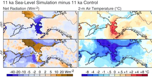
The impact of land-bridge flooding at 11 ka is illustrated by the 11 ka Sea-Level sim-ulation. Figure 6 shows the relationship between net radiation and temperature when

10

the land bridge is flooded (January and July anomalies for contrast). The major influ-ence on the energy balance comes from changing land to water, but the effects are not spatially uniform, as is the case for the present day land-bridge flooding experiment (Sect. 3.1). In Beringia, winter insolation is extremely low, and the January radiation balance is dominated by longwave radiation: incoming longwave radiation is relatively

15

constant but can be affected by circulation both within the RCM domain and through hemispheric circulation in the GCM, while outgoing longwave radiation is dependent upon surface properties and their respective temperatures, which here drive most of the observed variation. January net radiation anomalies show a strong dipole: positive north of Siberia (Laptev Sea) and negative over the land bridge (Fig. 6). This pattern

20

results from changing the present day shelf north of Siberia from land to sea ice which consequently has low surface temperatures throughout the year. Examination of other simulated variables indicates that this change results in decreased upward longwave radiation but little change in downward longwave radiation, and hence the mean diff er-ence in net radiation is positive. In contrast, in the ocean directly north and south of

25

(25)

CPD

11, 873–932, 2015

Title Page

Tables Figures

◭ ◮

Back Close

Full Screen / Esc

Discussion

P

a

per

|

Discussion

P

a

per

|

Discussion

P

a

per

|

Discussion

P

a

per

|

(greater upward longwave radiation). The difference in mean net radiation is negative, and thus surface temperature is relatively higher (see also Supplement Fig. 8b).

The net radiation dipole is absent in July (Fig. 6). While sea ice in the Chukchi and Bering Seas melts, the seasonal variation in temperature is strongly lagged. Even in July there is some sea ice present and temperatures are cooler than they would be

5

otherwise owing to its relatively high albedo. The ocean warms in late summer and fall as the ice reaches minimum extent, leading to the warmer January conditions de-scribed above. Overall, summer temperatures in the vicinity of the flooded land bridge are cooler than when the land bridge is in place.

3.3.2 Vegetation

10

The effects of changing vegetation from low tundra to a tundra-woodland mosaic on both sides of the land bridge produces modest warming with the clearest effect in May (Fig. 7). While upward longwave radiation is relatively high, net downward shortwave radiation is greater, a response to the lowered albedo of the wooded land surface, which leads to a positive net radiation balance. In May, an air temperature increase

15

of 1–2◦_{C (relative to the 11 ka Control simulation) is simulated over wooded areas,}

reflecting increases in sensible and latent heat fluxes. Substrate heat flux is lower as the land-atmosphere temperature gradient is reduced (Supplement Fig. 10b).

In winter (January) net radiation anomalies due to changed vegetation are small (Fig. 7). In tundra areas winter temperatures are slightly but consistently colder

reflect-20

ing less overall flow of heat to the ground and hence less upward longwave radiation in winter.

3.3.3 Lakes

Although the overall effect of placing lakes on the landscape is modest, it produces a clear pattern in summer (e.g., July: Fig. 8 top, Supplement Figs. 11 and 12) when

25

(26)

CPD

11, 873–932, 2015

Title Page

Tables Figures

◭ ◮

Back Close

Full Screen / Esc

Discussion

P

a

per

|

Discussion

P

a

per

|

Discussion

P

a

per

|

Discussion

P

a

per

|

Control simulation. For western Alaska, latent heat flux anomalies are positive in June and net radiation and sensible heat-flux anomalies are positive in June and July, and generally zero or negative the rest of the year (Fig. 8). For the entire study domain, the surface-temperature differences between the 11 ka Lakes simulation and the 11 ka Control simulation are substantial during April–August, and the accompanying changes

5

in atmospheric circulation are consistent with these differences (Fig. 8, Supplement Fig. 12). Positive sea-level pressure or 500 hPa height anomalies (e.g., April) reflect greater heating at the surface and consequent displacement of the circulation whereas the negative anomalies (e.g., July) reflect atmospheric cooling and subsequently lower and displaced 500 hPa height-anomaly patterns, particularly over the south-central

10

part of the land bridge where there are additional interactions with SSTs (Supplement Fig. 12). The overall impact of thaw-lake formation relative to that of vegetation is still small, however, and similar to that noted for “column-mode” simulations with an RCM under present day conditions (Rivers and Lynch, 2004).

3.3.4 All

15

The 11 ka All simulation shows the combined impact of all three land-cover changes (land-bridge flooding, vegetation change and thaw-lake formation). Figure 9 compares the monthly mean 2 m air temperature anomalies for changed vegetation, changed sea level and all land cover features changed together at 11 ka (see also Supplement Fig. 14). The vegetation change at 11 ka (Fig. 9a) acts to amplify the insolation effect,

20

making the whole year warmer, especially in early spring and summer (April through June), when there is greater absorption of incoming shortwave radiation relative to other times of the year or to the same time of year in the 11 ka Control simulation. This increased absorption leads to more heat storage in late summer, which carries over and is released during the winter season, thereby increasing upward longwave

25

radiation and causing a slight warming.

(27)

short-CPD

11, 873–932, 2015

Title Page

Tables Figures

◭ ◮

Back Close

Full Screen / Esc

Discussion

P

a

per

|

Discussion

P

a

per

|

Discussion

P

a

per

|

Discussion

P

a

per

|

wave radiation in winter (see above) the observed changes are modulated by albedo differences. The vegetation effect is overwhelmed by the sea-level effect through much of the year; it is only strongly expressed from April to June in the continental areas (Fig. 9c). The sea-level change acts to make winters warmer and summers cooler, countering the amplification of seasonality due to 11 ka insolation.

5

3.4 Principal responses other than temperature and energy-balance variables:

11 ka Control and 11 ka All vs. Present Day

During the interval from the LGM to present, the principal changes over the North Pa-cific and adjacent land areas in atmospheric circulation and variables that depend on circulation (i.e., clouds and precipitation) were governed largely by the retreat of the

10

North American ice sheets, with secondary influences from land-ocean temperature contrasts induced by insolation variations and ocean heat transport (Bartlein et al., 2014). In particular, when large, the ice sheets in GENESIS perturbed the upper-level winds, generating a “wave-number-1” (one circumpolar ridge-and-trough) pattern that resulted in stronger-than-present southerly flow over Beringia, while at the surface,

15

a strong glacial anticyclone developed. This circulation pattern results in the simulation of LGM near-surface air temperatures across much of the region that were as warm or warmer than present. By 11 ka, these e_ffects had greatly attenuated, but large-scale ef-fects on Northern Hemisphere circulation caused by the remnant ice sheet and greater land-ocean temperature contrasts in summer are apparent in the AGCM simulations

20

that provide the lateral boundary conditions for the RCM. As a consequence, relatively modest regional-scale modifications of the large-scale circulation might be expected in the different 11 ka RCM experiments. However, given the topographic complexity of the region even small changes in circulation could have large consequences on clouds, precipitation and soil moisture (although soil moisture is also governed by surface

25

(28)

CPD

11, 873–932, 2015

Title Page

Tables Figures

◭ ◮

Back Close

Full Screen / Esc

Discussion

P

a

per

|

Discussion

P

a

per

|

Discussion

P

a

per

|

Discussion

P

a

per

|

to late-summer and early autumn atmospheric circulation and moisture conditions than they are to contemporaneous wintertime conditions.

The impact of larger-scale circulation anomalies represented in the GCM can be seen in RCM simulations for Beringia (Fig. 10, also see Supplement figures). The anomalies with respect to the present day differ little between the 11 ka Control and

5

11 ka All simulations (Fig. 10a and b), and consequently can be discussed together. The anomalies also indicate that effects of the land-cover changes on regional cir-culation were small. In the 11 ka simulations, January 500 hPa heights are generally lower than present across the North Pacific, and higher than present over the south-eastern part of the domain, while at the surface, negative sea-level pressure

anoma-10

lies are centered over southwest Alaska and the Aleutian Islands. This pattern is somewhat analogous to the “January North-East Pacific Negative” pattern of Mock et al. (1998). As a consequence of the stronger-than-present southeasterly flow into eastern Beringia at both the surface and in the upper-atmosphere, cloudiness and pre-cipitation are greater than present in southern Alaska, while in eastern Siberia, stronger

15

than present offshore flow creates drier-than-present conditions. Soil moisture anoma-lies show a strong east (dry) to west (wet) pattern, which develops in October and persists through April.

In July, an east–west contrast in 500 hPa height anomalies exists (Fig. 10). Pos-itive anomalies occur in the western part of the region, where at present the East

20

Asian trough prevails, while negative anomalies occur over eastern Beringia, where at present a semi-permanent ridge develops. This anomaly pattern produces stronger-than-present zonal flow over the region that is consistent with the continued presence of negative (relative to present) 500 hPa height and sea-level pressure anomalies over the Arctic Basin upstream of the ice sheet and the developing enhancement of the North

25