Inequality treatment effects

P/EPGE SPE F527i

FUNDAÇÃO GETULIO VARGAS

,~

FGV

EPGE

:~

~~ ~-~-. .-

-

. . - - - -

---_._---_.-

,

SEMINÁRIOS DE PESQUISA

ECONÔMICA DA EPGE

Inequality treatment effects

SERGIO FIRPO

(PUC/RJ)

Data: 05/05/2005

(Quint~-feira)

Horário: 16h

Local:

Praia de Botafogo, 190 - 110 _andar

Auditório nO 1

Coordenação:

Prof. Luis Henrique B. Braidcie-mail: Ibraido@fgv.br

:, ...•

Inequality Treatment Effects*

Sergio Firpo

t

First draft: July 2003; This version: February 2005

Abstract

This paper presents semiparametric estimators for treatment effects parameters when selection to treatment is based on observable characteristics. The parameters of interest in this paper are those that capture summarized distributional effects of the treatment. In particular, the focus is on the impact of the treatment calculated by differences in inequality measures of the potential outcomes of receiving and not receiving the treatment. These differences are called here inequality treatment effects. The estimation procedure involves a first non-parametric step in which the probability of receiving treatment given covariates, the propensity-score, is estimated. Using the reweighting method to estimate parameters of the marginal distribution of potential outcomes, in the second step weighted sample versions of inequality measures are.computed. Calculations of semiparametric effciency bounds for inequality treatment effects parameters are presented. Root-N consistency, asymptotic normality, and the achievement of the semiparametric efficiency bound are shown for the semiparametric estimators proposed. A Monte Carlo exercise is performed to investigate the behavior in finite samples of the estimator derived in the paper.

JEL: Cl, C3 Keywords: Treatment Effects, Inequality Measures, Semiparametric

Effi-ciency, Reweighting Estimator

• An earlier version of this paper circulated under the name "Treatment Effects on Some Inequality Measures" .

This paper reflects part of my Ph.D. dissertation at UC Berkeley. I am indebted to Guido Imbens and to Jim

Powell for their advice, support and many suggestions. I have also benefited from comments from participants

at the 2004 Meeting of the Sociedade Brasileira de Econometria and at the empirical lunch seminar at UBG.

FinanciaI support from CAPES - Brazil and UBC's Start-Up Research Grant is acknowledged. All errors are

mine.

tThe University·ofBritish Columbia and PUC-Rio. Mailing address: University of British Columbia,

1 Introduction

In evaluating a social program the policy-maker may want to learn not only about the mean

effect of the program, but aIs o about its distributional effects. For example, it would be

reason-able to assume that the policy-maker is interested in the effect of the treatment on the dispersion

of the outcome, which can be captured by inequality measures such as the Gini coefficient, the

quantile-ratio, the interquartile range and many other inequality indices. One way of computing

the distributional effect of the social program is through the inequality treatment effects (ITE) ,

defined here as differences in inequality measures between the distribution of potential outcome

of joining the program and the distribution of potential outcome of not joining it.

The program evaluation literature has not typically focused on inequality measures, or

more generally, on distributional characteristics of program impacts.1 A good reason for that is because treatment effects have been in most cases associated with individual treatment effects,

defined as the difference in the individual potential outcome of joining the program and the

potential outcome of not joining it.

However, it is very well recognized that the cenüal identification problem in the program

evaluation literature is that individual treatment effects are never observed, as an individual

either receives the treatment or noto This is true even when the interest relies on the most

popular treatment effect parameter, the average treatment effect (ATE), which identifies the

individual treatment effect only if there is no heterogeneity in the effects, what may be a very

strong assumption in many cases. Other treatment effect parameters, such as the quantile

treatment effects (QTE), have received less attention, as their interpretability in terms of

indi-vidual effects is less clear than it is for the mean case.2 Nonetheless, there are many relevant

aspects for policy purposes that are related to effects of social programs on the distribution of

the outcome, a fact that weakens the sole interest in individual effects of those programs.

Unlike many other fielâs' in economics, the welfare economics literature has had a long

standing interest in the measurement of income inequality. Inequality measures can be justified

lSome exceptions are the papers by Imbens and Rubin (1997), Abadie, Angrist and Imbens (2002), Heckman,

Smith and Clements (1997) and, more recently, Firpo (2004). In the applied literature a recent paper that focus

on the treatment effect of a social program on the income distribution is Bitler, Gelbach and Hoynes (2004). 21ndividual interpretation of QTE requires the assumption that individuaIs would keep their rankings in the

both the distributions of the potential outcome of being treated and of not being treated. Such discussion can

be found in Firpo (2004), Bitler, Gelbach and Hoynes (2004) and Heckman, Smith and Clements (1997).

2

either as a parameter in the social welfare function or from a ad hoc perspective. Many popular

inequality measures do not result from an utilitarian point of view and are instead built based

on the satisfaction of some desirable properties. Among those properties, the most common

and important ones are the principIe of transfers, invariance, decomposability and anonymity.3

Anonymity means that inequality measures should not change if we are able to just

re-label individuaIs, as this operation does not to alter the distribution of income. This property

is shared by alI inequality measures that are based solely on the overalI income distribution.

Examples are alI the usual inequality measures, such as the variance, quantile ratios and ranges,

the Gini coefficient and several others.

The typical set of assumptions used primarily to identify treatment effect parameters does

not, however, alIow identification of the joint distribution of potential outcomes. Therefore,

assessing individual impacts of social programs is not generally feasible.4 _{That set of}

assump-tions is calIed the ignorability of the treatment.5 _{This assumption is a conditional independence}

assumption: Given observable characteristics, the decision to be treated is independent of the

potential outcomes associated with being treated and with not being treated. This is also

known as the selection on observables assumption and it makes possible to identify the

mar-ginal distributions of potential outcomes.

It is therefore c1ear that we can combine the genuine interest of the welfare economics with

the "limitations" of the program evaluation literature. In this paper, the welfare economics

literature and the program evaluation literature are combined and we establish conditions for

identification and show how to estimate treatment effects on summary parameters of the

out-come distribution.

This paper is divided as follows: In the next section we present a simple economic model

of treatment effects on distributions that provides a theoretical justification for the interest in

the inequality treatment effects. Section 3 presents the main identification result of this paper.

Section 4 discusses estimation and derive the large sample properties of the inequality treatment

effects estimators. In that section we show that "natural" estimators of the treatment effects

3See Cowell (2000) and Cowell (2003).

4 An important exception happens when we are interested in a parameter that is a linear operation of the

treatment effect distribution. This is exactly the case of ATE: the mean of the difference in potential outcomes

on inequality measures are two-step type estimators. We show that these are root-N consistent

and asymptotically normal. We aIs o calculate the semiparametric efficiency bounds and show

that the proposed estimators achieve them. Section 5 discusses finite-sample behavior through

a Monte Carlo exercise. Finally, section 6 conc1udes. Proofs of results are left to the Appendix.

Along part of this paper we apply the general theory developed here to two particular cases:

the variance and the 75-25 inter-quartile range (the difference between the 75th and the 25th percentiles). Note first that these two examples were chosenbecause they are very illustrative

of how broad the methodology presented here can be: while one is an expectation parameter,

the other is a function of quantiles. Other inequality measures fit the framework developed

here, like the Gini co eflicient , those in the Generalized Entropy Class and many others. AIso,

the approach developed here is broad enough to subsume other parameters of the distribution

of the outcome, such as the mean and quantiles. In that sense, ATE and QTE could be seen

as particular cases of this method.6

2

A Simple Model of Treatment Effects on Distributions

In this section we present a sim pIe model that have two important features that justify the

interest in the treatment effects on distributions: First, the individual decision to be in the

treatment group depends on a vector of observable covariates and, second, the policy-maker

aims to learn features of the marginal distributions of potential outcomes.

We start by assuming that there is an available random sample of N individuaIs (units). For

each unit i, let Xi be a random vector of observed covariates with support X C ]RT. Define Yi(l)

as the potential outcome for individual i under treatment, and Yi(O) the potential outcome for the same individual without the treatment. Let the treatment assignment be defined as Ti,

which equals one if individual i is exposed to treatment and equals zero otherwise. As we

only observe each unit at one treatment status, we say that the unobserved outcome is the

counterfactual outcome. Thus, the observed outcome can be expressed as:

Yi = liYi(l)

+

(1 -li)Yi(O), Vi. (1)

6 Recently, Chen, Hong and Tarozzi (2004) have independently showed that using a similar set of identifying

assumptions, the approach of this paper could be generalized to a broader class of problems, such as missing

data and non-classical errors in variables.

4

To motivate, consider Yi as the observed earnings of individual i in a model of the impact of a job training program on worker earnings. In this example, Ti is the indicator for the receipt

of training.

Potential outcomes depend on both observed and unobserved individual characteristics. For

each individual i, let Ci be a vector of unobservable attributes. In a job training program model,

for example, earnings of each individual are a function of their pre-program observable

charac-teristics, such as past earnings, employment status, education, age, job experience, gender, and

union status; they are also a function of unobservable attributes, such as ability, motivation

and some possible idiosyncratic shock.

Suppose the impact of X and c on the potential outcomes is given by:

Yi(l) = G1 (Xi, ci)

Yi(O) = GO (Xi, ci)

(2)

(3)

We assume self-selection into treatment: individuaIs can decide whether or not to be treated.

When an individual i faces the decision whether or not to join the job training program, he will weigh the gains and costs of both situations. Assume that an individual i predicts his (or her) expected earnings (given his vector Xi) and his (or her) costs for each of the alternatives. In

other words, the individual i chooses the state that yields the largest expected utility:

where u(·) is utility function, C1 (·,·) and Co(-,·) are some costs associated respectively with

joining the training program and not joining it, and TJi is a vector of variables that is unobserved

to the econometrician but not to the individual. AIso, TJi is assumed to be independent of

Ci· The effect of TJi on the individual's utility will depend on whether or not he enters the

job programo For example, TJi might be a reservation wage that enters as an argument to

a foregone earnings function. Individual i will then--choose to take part in the program if

E[u(Y(l))

I

Xi,

TJil -

C1 (Xi, TJi)

2:

E[u(Y(O))

I

Xi,

TJil-

CO(Xi, TJi). That iS:7

(5)

Note how this model fits into the Roy model (1951) of income distribution.~ In the Roy

7The indicator function ll{A} is equal to one if Ais true and zero otherwise.

model, an individual chooses the largest of the potential earnings given by two different

occu-pations. Here, the choice is based on the individual's expected earnings and on some individual

cost. Thus, after controlling for Xi, the choice of getting treatment will be independent of the

individual potential earnings, which depends only on Xi and êi. That will hold as long as TJi

and êi are independent and the functional form of potential earnings is the one described in

Equations (2) and (3). The independence result can be written as:

(Yi(l), Yi(O)) Jl Ti

I

Xi Vi (6)

Equation (6) is the unconfoundedness (or ignorability) assumption labeled by Rubin (1977).

Unless there is a gain in insight to writing the model with the structure presented in Equations

(2)-(5), Equation (6) could actually have been our starting point.

Assume now that there is a social welfare function, W, that depends on a vector 1/ of

parameters of the earnings distribution. We can write 1/ as a real function of the earnings

distribution, that is, letting Fl/ be a class of distribution functions such that F E Fl/ if 1/ (F)

<

+00, we define 1/ : Fl/ -+ IR.. An example of W and 1/ is the case where 1/ is an inequality

measure and W its inverse: The smaller the inequality the larger the welfare.

In order to simplify the argument, imagine that there are two possible scenarios: we either

treat everyone or treat no one.9 Under the first scenario, the distribution of earnings is then equal to distribution of Y(l), which has the distribution function FY(l); while in the second

scenario, the earnings distribution equals that of Y(O), whose distribution function is Fy(o).

We define the Inequality Treatment Effect, ~l/' as:

which is the difference in outcome (earnings, in this example) inequality between providing

everyone the training and not providing it at alI. Other parameters could be defined to

sub-populations. In particular, consider the Inequality Treatment Effect on the Treated,

~l/IT=l:

where FY(l)IT=l and FY(O)IT=l are respectively the conditional distribution functions of the potential outcome of being treated and of not being treated given the treatment.

Y Alternatives, as discussed in Manski (1997), include allowing individuais to choose their treatment status or

assigning them to treatment based on observed characteristics.

6 ' \

-,

!

"

3

Identification of Inequality Treatment Effects

We now set up assumptions for identification of .6.v . Remember that because Y(l) and Y(O) are

never fully observable, we need to impose some identifying assumptions for parameters based

on their marginal distributions, such as .6.v is. Before doing so and giving sequence to the

definitions, let us define the "propensity-score", p( x), as the probability that, given a value x

of X, an individual will be in the treatment group, that is, p(x)

=

Pr[T

=

11X = x]. The

unconditional probability is p, which will be assumed to be positive.

Now we are able to state and discuss the following assumptions.

ASSUMPTION 1 [Ignorability] Let (Y(l), Y(O), T, X) have a joint distribution. For ali x in X:

(Y(l), Y(O)) is jointly independent from T given X = x, that is, (Y(l), Y(O)) lL T

I

X = x.

This assumption has become popular in empirical research after a series of papers by Rubin

and coauthors and by Heckman and coauthors10. Assumption 1 should be analyzed in a case-by-case situation, as for many exercises it is plausible not to hold.

We aIs o make an overlap assumption:

ASSUMPTION 2 [Common Support] For all x in X, 0< p(x) < 1.

Under Assumptión 2 there is overlap in observable characteristics across groups, in the sense

that it does not exist a value of x in X such that it is only observed among individuaIs of one

of the groups.

Another necessary assumption for identification is uniqueness. This can be written as:

ASSUMPTION 3 [Uniqueness] Let F A and FB E Fv where Fv is a class of distribution functions

such that F E Fv if v (F)

<

+00.

lf FA = FB then, V(FA) = V(FB) .

Finally, the main identification result will follow as a corollary of the next lemma.

LEMMA 1 Let FY(l)(y), Fy(o)(y), FY(l)IT=l(y), and FY(O)IT=l(y) be the respective cumulative

distribution functions (c.d.f.) of Y(l), Y(O), Y(l)IT

=

1, and Y(O)IT

=

1 evaluated at a real

IOSee, for instance, Rosenbaum and Rubin (1983 and 1984), Heckman, Ichimura, and Todd (1997) and

number y. Under Assumptions 1 and 2 these c.d.f.s can be expressed as:

COROLLARY 1 Under Assumptions 1, 2 and 3, _{6. v} and _{6. v1T=1} are identifiable.

Once we know that those inequality treatment effects are identifiable, we can now turn our

attention to estimation and inference.

4

Estimation and Asymptotically Valid Inference

We now focus our attention to estimation of li (FY(l)) as estimation and inference of li (Fy(o)) ,

li (FY(l)IT=l)' and li (FY(O)IT=l) follow by analogy. As the main objects of this paper are

6. v

=

li (FY(l)) - li (Fy(o)) and 6. v1T=1

=

li (FY(l)IT=l) - li (FY(O)IT=l).,.after we show how to

estimate and derive the asymptotic distribution of the estimator of li (FY(l)) ' we will also show

how those results can be extended for estimation and inference regarding 6.v . An extension to

6. vIT=l is not presented here although it would easily follow by analogy.

4.1 Estimation

Estimation of li (FY(l)) follows from the sample analogy principIe, as the empiricaI distribution

function of Y(1) can be written as FY(l) (y) =

Jv

L:{:l pc};) ·ll{Yi:S y}. The key step that can be noticed is estimation of the propensity-score by

pU.

As argued before, this is done in a first step, which we explain now.

Start by defining HK(X)

=

[HK,j(X)] (j

=

1, ... , K), a vector of Iength K of poIynomiaI functions of x E X satisfying the following properties: (i) _{HK :} X _lRK; and _{(ii) HK,} l(X) = l. If we want H K( x) to include polynomiaIs of x up to the order n, then it is sufficient to choose

K such that K ~ (n

+

1)R. In what follows, we will assume that K is a function of the sampIe

size N, K = K(N) -

+00

as N -

+00.

8

.' -\

'I'

Next, the p(x) is estimated. Let p(x) = L(HK(X)'ir), where L : lR -+ lR, L(z) (1

+

exp(-z))-l; and

N

ir = argm;x

~

L

(Ti log(L(HK(Xd'7f))

+

(1 - Ti) log(l- L(HK(Xd7f ))) .

i=l

Also, when we need to estimate p, the unconditional probability of being treated, we consider

the simple estimator

p=

EI:l

Ti/N.

The second step follows a reweighting argumento The estimator of vY(l)

=

v (FY(l)) is

í/Y (1) = v (FY(l) ). It can be computed as one would compute any inequality measure using

data from the empirical distribution of Y, the only difference is the necessary usage of the

weights p(l;). As examples, consider the following two inequality measures, the variance and

the 75-25 inter-quartile range.

Example 1: Variance. The variance of Y(l), v~(l)' can be written as:

However, as the distribution of Y(l) is not observable, under assumptions 1-3, the reweighting

scheme will be used to write v~(l) as

(7)

and its estimator as

(8)

Example 2: The 75-25 Interquarlile Range. Even when the inequality measure is not an

expectation,

as

the variance is, we can apply the reweighting method. The interquartile range

is an example of such case. Fortunately, we can use the results derived in Firpo (2004) to

express the 75-25 inter-quartile range of the distribution of Y(l),

v;'6f

5,

as:

V75- 25

Y(l) qY(1),.75 - qY(1),.25

= argmJnlE [p

~)

. (Y - q)(.75 - lI{Y - q :::; O})]

- argmJnlE

[p

~)

.

(Y -

q)

(.25 -II{Y -

q:::;

O})] ,

and its estimator is defined as:

4.2 Inference

QY(1),.75 - QY(1),.25

1 N

T

argmin N

L

~(;.)

.

(Yi - q) (.75 -II{Yi

-q:S

O})

q i=i P ~ N

- argmin

~

L

~

Tj . (rj - q) (.25 -II{Y .-q

:s

O}) .

q N j=i p(Xj ) J

(10)

We now devote our attention to the asymptotic behavior of our estimators. This subsection is

divided in the following parts. We first show how to estimate the first step, that is, how the

propensity-score function is estimated. Then, we invoke the hypothetical case of full

observ-ability of potential outcome to establish conditions for asymptotic normality and efficiency of

our estimators, which are shown in part 3. Finally we show how to consistently estimate the

standard errors of our estimators.

4.2.1 The First Step

An important assumption for the final ITE estimators to be asymptotically normal are that

the first step estimator of the propensity score be uniformly consistent. In order to guarantee

uniform consistency of this first step procedure, we assume that:

ASSUMPTION

4

[Distribution of X and Smoothness] (i) X is a compact subset ofIRr; (ii) the density of X, f(x), satisfies O

<

infxEx f(x)

:s

sUPxEX f(x)

<

00 (iii) p(x) is s-times

continuously differentiable, where s

2::

7r and r is the dimension of X; (iv) the order of HK(X),

K, is of the form K = C . NOi where C is a constant and Q E

(4.</-1)' à).

Newey (1995, 1997) established that for orthogonal polynomials HK(X) and compact X,

((K) = sUPXEX

IIHK(X)II

:s

C· K, where C is a generic constant. Note then that because of

part (iv) of Assumption 4, ( will be a function of N since K is assumed to be a function of N.

Following Hirano, Imbens and Ridder (2003), we can invoke state the following result:l l

LEMMA 2 Under Assumptions 1 and

4

the following results hold: (i) sUPXEX Ip(x) - PK(x)1

:s

C· ((K)K-s/ 2r

:s

C· (1-s/2r

:s

C· N(1-s/2r)Oi

=

0(1); where PK(X)

=

_{L(HK (x)T 7rK ) and}

11 Renceforth sometimes we wilJ refer to their paper as RIR.

10

, "

7rK = argmaX7rlE{p(x) log(L(HK(X)T7r))

+

(1 - p(X)) log(l - L(HK(X)T 7r ))}; (ii)

lEllft-7rKW ::; C·

çcç:) ::;

C· Ncx- 1 = 0(1); (iii) there is Ó

>

O: limN->= Pr[Ó

<

infxEx p(X)

<

SUPXEX p(X)

<

1 -

ÓJ

= 1.

An important point to make here is that Assumption 4 is stronger than the necessary for

Lemma 2 to hold. This can be seen more clearly in the proof by RIR. In fact, the condition

that s ~ 7r is too strong for unifom consistency of the first-step: 4r times differentiable would

be enough. Assumption 4 is maintained though as it is necessary for the asymptotic normality

of the final estimators of the inequality treatment effects.

4.2.2 A Hypothetical Benchmark Case: Full Observability of Potential Outcomes

We will need to establish some extra conditions to be able to derive the asymptotic normality

of the inequality estimators just proposed. Among those conditions, two are presented now:

That their influence functions under the hypothetical case of fuH observability of potential

outcomes have (i) finite variances and (ii) continuously differentiable conditional expectations

given X = x.

Let us now define 'lj;y (y; 8y,Y(1)) as:

( . ) _ dll((l-s).FY(1)+s.Óy)

'lj;y y,8y,Y(1) - d S

15=0,

(11)

where Óy denotes the c.d.f. of the degenerated distribution that places probability one at the

point y. The function 'lj;y (y; 8y,Y(1)) is then the derivative with respect to s of lI((l - s) . F_Y(1) +s . Óy ) evaluated at s = O, or said in another way, it is the Gâteaux derivative of li (-) at y. It

is also an influence function associated with the parameter lIY(l) under the assumption of full

observability of Y (1).12 The vector 8y,Y(1) is a parameter vector that takes values from the

distribution FY(1) to JRL and includes lIY(l). By analogy, 'lj;y (.; 8y,Y(0)) is an influence function

of the parameter lIy(O) under the assumption of fuH observability of Y (O).

Now, we state some assumptions regarding the variance and the conditional expectation

given

X

of 'lj;y

(Y

(1) ; 8y,Y(1)) and 'lj;y

(Y

(O) ; 8y,Y(0)).

12The influence function of an estimator places a key role in the robust statistics literature, so the natural

. -.. --- _ _ ~~'""" _ _ _ _ _ _ _ T~ _ _ _ _

ASSUMPTION 5 [The lnftuence Punction] Assume that:

(i) E [(1/111 (Y(1);OIl,Y(I»))2]

<

(Xl and E [(1/111 (Y(0);OIl,Y(O»))2]

<

(Xlj

(ii) E [1/111 (Y(l); OIl,Y(I»)

I

X

=

x] and E [1/111 (Y(O); OIl,y(O»)

I

X

=

x] are continuously

differ-entiable for all x in X.

The above assumption is crucial for the derivation of our limiting distribution theory. Part

(i) is the usual condition of square integrability of the influence function, whereas part (ii) is

a regularity condition used in bounding a remainder termo As we will see in the proof of the

main theorem of this paper, Assumption 5 plays the same role that HIR's Assumption 3 plays

in the proof of their Theorem 1.

Given the generality of the parameters in this paper, for the analysis of the asymptotic

behavior of their estimators we will restrict ourselves to a specific class of parameters. Under

full observability of potential outcomes, we will assume that each parameter in that class will

be estimated by an asymptotically linear estimator whose influence function lies on the tangent

space of the statistical model (under full observability of potential outcomes). Furthermore, 1/

will be assumed to be pathwise differentiable, that is, 1/1 will be the efficient influence function

of 1/. Before we state more formally these points as assumptions, let us first define S[ULLand

S[ULL the tangent spaces of the models under full observability of potential outcomes, as

S[ULL = {SI: IR x {O, 1} x X - t IR

I

SI(Y, t, x) = SI(Y, Ix)

+

a(x)· (t - p(x))

+

sx(x); such that

E [SI(Y (1) IX)] = E [sx(x)] =

°

and a(x) is square-integrable function of x}

and

S[ULL

=

{So : IR x {O, 1} x X - t IR

I

So(y, t, x) = so(y, Ix)

+

a(x)· (t - p(x))

+

sx(x); such that

E [so(Y (O) IX)] = E [sx(x)]

=

°

and a(x) is square-integrable function of x}.

AIso define WI = [Y (1) ,T, XTF and W

o

= [Y (O) ,T, XT]T. Under this terminology, we define

LlII as:

LlII = 1/ (p.

J

dFw1 (',l,x)dx+ (l-p)·

J

dFw1 (.,O,X)dX)

-1/ (p.

J

dFwo (',1, x) dx

+

(1 - p) .

J

dFwo (-,0, x) dX)

AIso, we define the estimators under the hypothetical case of full observability as functionals

of the follciwing empirical distributions, which have the superscript U, as in "unfeasible", to

remind us that the potential outcomes are in reality never observed. They are:

F-Ç:!(1)

(Y)

12

.----1

__ o,

"

,"-, )

_ 1 N ~U

- N 2:i=l1[{Yi (1):::; y} and Fy(O) (y)

v

(F~(O))'

We are now ready to state two key assumptions for our asymptotic results:

ASSUMPTION 6 [Asymptotic Linearity of Unfeasible EstimatorJ We assume that if

ran-dom samples of

{Yi

(1), Ti, Xi} and

{Yi

(O) ,Ti, Xi} were available then, Li~ would be a regular estimator of /:).// such that:

N

Li~

- /:).// -

~

2::

(~//

(Yi

(1); 9//,y(l)) -

~//

(Yi

(O); 9//,y(o))) = op(1jVN).

i=l

AIso, we consider that the following assumption holds:

ASSUMPTION 7 [Efficiency of Unfeasible EstimatorJ Let FWl (w;9) and Fwo (w;9) E F//

be model such that their tangent spaces are respectively characterized by S[U LL and SÕU LL .

We assume that: ~// _{(-; 9Y (l))} E S[ULL and ~// (-; 9 y (o)) E SÕULL .

Although apparently too restrictive, assumptions 6 and 7 are noto Consider the examples

already given, the variance and the 75-25 interquartile range.

Example 1: Variance (continued). The unfeasible estimator of the variance is defined as:

~VU 1

N (

1

N)2

v

_Y

(l) = N

~

Yi

(1) - N

f;Yj

(1) ,

and we can verify that

N

íliK) -

Vh1) -

~

2::

((Yi

(1) - E [Y (1)])2 -

V~(l))

i=i

N

_ ~v,u v 1 ~ v ( . ( ). 9 ) _

(j r;:;)

- vY (l) - vY(l) - N ~ ~//

Yi

1 , Y(l) - op 1

v

N ,

which will hold by the fact that under full observability of Y (1),

k

2:f:i

Yi

(1) -E [Y (1)J

= op (1). Therefore, applying the same results to Y (O), we have that:

N

Li~,u

-

/:).~

-

~

2::

(~~

(Yi

(1) ; 9 Y (l)) -

~~

(Yi

(O) ; 9 y (o))) = op(1jVN).

i=l

AIso, ~~ (-; 9//,Y(l)) E S[ULL and ~~ (.; 9//,y(o)) E SÕULL as such examples fit into Example 3.3.2 and Proposition A.5.2 of Bickel, Klassen, Ritov and Wellner (1993).13

~I

_,

Example 2: The 75-25 Interquariile Range (continued). The same is true for interquartile (

range. To see that, note that the unfeasible estimator for Y (1) is defined as:

~75-25,U = ~ ~

lIY (l) qY(1),.75 - qY(1),.25

1 N

= argmjn N ~ (ti (1) - q) (.75 -lI{Yi (1) - q ~ O})

t=t

1 N

- argmin N

L

(Yj (1) - q) (.25 - lI{Yj (1) - q ~ O}) .

q "

J=t

And then,

~75-25,U 75-25

lIY (l) - lIY (l)

_

~

N ((.75 -lI{Yi (1) -

(1I~(~)5

+

qY(1),.25)

~

O}) _

(.25 -lI{ti (1) - qY(1),.25

~

O}))

N

L

_i=i

(

7 5 - 2 5 )

f

(q

)

fY(l) lIY (l)

+

qY(1),.25 Y(l) Y(1),.25

N

_ ~75-25,U 75-25 1 "Ç""., 75-25

(1': ( ).

O ) _ ( /

'ii)

- lIY(l) - _{lI Y (l) -} N L '/)" t I , Y(l) - op 1 v lV

i=l

where O",Y(l) = [1I~(~)5, qY(1),.25]T. We assume that fY(l) (qY(1),.75)

#-

O and fY(l) (QY(1),.25)

#-O. The above equation will hold as a result from an application of the ordinary delta-method to

the difference ~(1),.75 - ~(1),.25' where for T = {.25, ,75}, as showed, for example, in Corollary

21.5 of van der Vaart (1998),

1

~

(T-lI{Y(l)-QY(l),T:S;O})

(r;;r)

= QY(l) T

+ -

L

+

op

l/v

N

, N i=l fY(l) (QY(1),T)

1 N

QY(l),T

+

N

L

'!f;"q (ti (1); QY(l),T)

+

op

(l/Vii) .

i=l

Also, one can check that '!f;"q (-; QY(1),.25) and '!f;"q (-; QY(1),.75) lie on the tangent space S{ULL

and furthermore, that QY(1),.25 and QY(1),.75 are pathwise differentiable (as in BKRW's Definition 3.3.1). Thus, as an application of Proposition 3.3.1 and Corollary 3.3.2 of BKRW, í/~(~~5,U will be asymptotically efficient under fuIl observability of Y (1).

4.2.3 Asymptotic Normality and Efliciency

Let us now define some objects that we wiIl see are important in getting an expression for the

asymptotic distribution of the estimators

L5.".

.----~---~~~- - - -- - - -- - - -- - -

-where

T ( 1-T )

<PJj. (Y, X, Tj ()v) = p (X) . '1f;v (Yj ()v,Y(l») - 1 _ p (X) . '1f;v (Yj ()v,y(O») ,

and

Cl:'Jj. (T,Xj()v) =

_ (E

['1f;v (Yj ()v,Y(l»)

I

X, T

=

1]

+

E

['1f;v (Yj ()v,y(O»)

I

X, T

=

O]) .

(T _ (X)).

p(X) 1 - p(X) P

where ()v = [()v,Y(l),()v,Y(O)]T.

Some words about the previous functions. As will be stated in the next theorem, the

function '1f;Jj. and is the infiuence function of the estimator

.6.

_v. It is a sum of two functions: <pJj.

and Cl:'Jj.. When the parameter LI is an expectation, then the first term can be interpreted as the

function generating the moment condition: .6._{v -} E [<pJj. (Y, X, Tj ()v)]

=

O.

The Cl:'Jj. function represents the effect on the infiuence function of estimating p(.). Its first

I . l' . f (E[1/Jv(Y;9v Y(l)) I X,T=l] E[1/Jv(Y;9v Y(Q)) I X,T=O]) . h d" 1

mu tlp 1cat1ve actor -_{, p(X)} '

+

_l-p(X)

'

_' lS t e con ItlOna

ex-pectation of the derivative of with respect to p( x). Hence, the function '1f; Jj. linearizes the effect

of the propensity-score, p (x).

Finally, define:

E [('1f;Jj. (Y, X, Tj

()))2]

= E [(<pJj. (Y, X, Tj ()v)

+

Cl:'Jj. (T, Xj ()v))2]

E[V ['1f;v (Yj()v,Y(l») IX,T=l]

+

V ['1f;v (Yj()v,y(O») IX,T=O] (12)

p(X) 1-p(X)

+

(E

[;bv (Y; Ov,Y(l»)

IX,

T =

1

J

-E

[;bv (Y; Ov,Y(O»)

I

X,

T =

O])'].

We are now ready to establish the key inference result of the papeI.

THEOREM 1 Under Assumptions 1-6:

(i)

..JN

(.6.

v -.6.v) =

JN

~:l

'1f;Jj. ()li, Xi, Tij ()v)

+

op(l)

~

N

(O,

O"~J

(ii) and adding an extra condition, Assumption 7,

O"L

is the semiparametric efficiency bound

4.2.4 Variance Estimation

The variance term

O"t

can be estimated by replacing expectations by sample averages. There

are two important points in the variance estimation procedure. One has been addressed by

RIR and is the fact that the a function depends on conditional expectations that need to be

estimated, and following their approach, we use the same type of estimation that we used in

the estimation of the propensity-score. The other point, which, unlike RIR is relevant for our

case, is that both the cp function and part of the Ov parameter might need to be estimated as

well. Thus, the estimator for the bound

O"t

will be:

where Ô_{v is an estimates of Ov of the type:}

and where

cp

~ is the following estimate of cp ~:

cp~

(li,

Xi,

Ti;

Ôv) =

P~i)

.

:;j;v

(li;

ÔV,Y(l)) -

(1

~ ;~i))

.

:;j;v

(li;

ÔV,Y(O)) .

The function

â~

(T,

X;

Ô

v ) is:

The 7jJv function considered here converges pointwise in probability to 7jJv' We state that as the

following assumption:

ASSUMPTION 8 [Consistency of the "Proxy" for the Inftuence Punction] Assume that

(i) :;j;v

(y,

OY(1)) -7jJv

(y,

OY(l))

=

op (1) for any

y

in the support of Y(l); (ii) :;j;v

(y,

ÔY(O))

-7jJv (y,OY(O)) = op(l) for any y in the support of Y(O); and 7jJv(',') is continuous in its

second argument at OY(l) and OY(O)'

16

Consider now the examples already discussed, the variance and the interquartile range. We

can see in both cases, computation of

ê

v , cp!::. and li!::. can be performed by the following way:

Example 1: Variance (continued):

p(x)

((y -

~t.

p(;j) .

Y} -

");(1))

- (1

~

;

(x) ) . (

(y -

~

t.

(1

~ ;(~,))

.

'í )

2 -");(0)) .

and

Notice that in this case, the function

:;jvv (-,.)

is exactly equal to

'l/Jvv (.,.)

thus, in order to

check whether Assumption 8 holds, we just have to be concerned about (a)

'l/Jvv (.,.)

being

continuous in its second argument at the true value of () and (b)

ê

v - ()v = op (1). But (a) and

(b) can be easilyverified to hold in this caSe.

Example 2: The 75-25 InterquaTtile Range (continued):

~() [~ ~75-25 ~ ~75-25] T

aIs o

~

( .

~

) _ t .

((.75 -

lI{y-

(í/~6)5+qY(1),.25)

~

O})

'Pb. _, 75-25 y, X, t, (}v75- 25 - _P ~( ) ~ ( )

X

f

~75-25 ~

Y(l) ZlY(l) +QY(1),.25

and finally:

_ (.25 -

~1I{y-qY(1),.25

~

O}))

fY(l) (qY(1),.25)

_ ( 1

-=

t ) .

((.75 -

lI~y

-

(í/~(O)5+qY(O),.25)

~

O})

1 - P (x)

f

(~75-25 ~ )

Y(O) Zly(O) +QY(O),.25

_ (.25

-~1I{y-qY(O),.25

~

O}))

fy(o) (qY(O),.25)

where Ôv75-25 was previously defined, and fY(l) (y) and fy(o) (y) are estimated similarly as in

DiNardo, Fortin and Lemieux (1996) as:

N

~

I""

Ti 1 } i - y

fY(l) (y) = N L ~(X·) .

h .

K(-h-) i=l P ~

~

1~(

l - T i )

1

}i-y

fy(o) (y) = N

ti'

1 - p(Xi) .

h .

K(-h-)

where K(·) is a kernel function and h is a bandwidth. Under typical conditions for (a) kernel

density estimation to be consistent; (b) the estimators í/~(1)5 and QY(1),.25 to be consistent for

ZI~(1)5 and QY(1),.25, Assumption 8 will hold for this case.

We now state the result regarding the consistency of the variance estimator.

THEOREM 2 Under Assumptions 1-8,

ô'i., -

a~v = op (1).

18

·1

...

-/ J

.-5

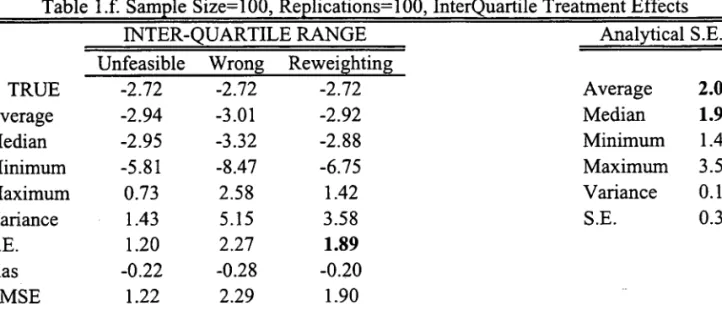
A Monte Carlo Exercise

In this section we report the results of Monte Carlo exercises. The interest is in learning how the

estimators for the overall inequality treatment effect (OITE) and estimators of their asymptotic

variances behave in finite samples. The generated data follows a very sim pIe specification:

X

=

[Xl, X2]T rv Bivariate N([J.Lxl' J.LX2]T, n

x ),

T

=

1I{00 +OlXl +02X2 +03xí +7]

>

O} where

7] has a standard logistic c.dJ. F7J(n) = (l+exp(-7rn/J3))-\ Y(O) = (hXl + 82 X 2 +'Oê

and Y(I) =

f3

+ 8lXl + 82X2 + 11ê, where ê is distributed as N(J.Le, i7~). The variables X, 7],

EO and E1 are mutually independent. The parameters were chosen to be: J.LXl = 1, J.LX2

=

5,

n X,l1

=

i7~1

=

1, nX,22

=

i7~2

=

1, n X,12

=

i7Xl.X2

=

O, 00

=

-1, 01

=

5, 02

=

-5, 63

=

-.05, 81

= -

5, 82

=

1,

f3

=

5, _J.Le

=

O, i7~

=

1, 10

=

5 and I I

=

.5. Under this specification,

Y(I) rv N (5, 26.25) and Y(O) rv N (O, 51). This specification leads to selection on observables,

and estimation of treatment effects not taking the selection into account will inevitably produce

inconsistent estimates.

One hundred replications of this experiment with three different sample sizes were

consid-ered: 100, 1,000 and 10,000 observations. As Y(I) and Y(O) are known for each observation

i, we can also compute "unfeasible" estimators of parameters of the marginal distributions of

Y(I) and Y(O).

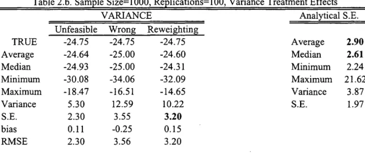
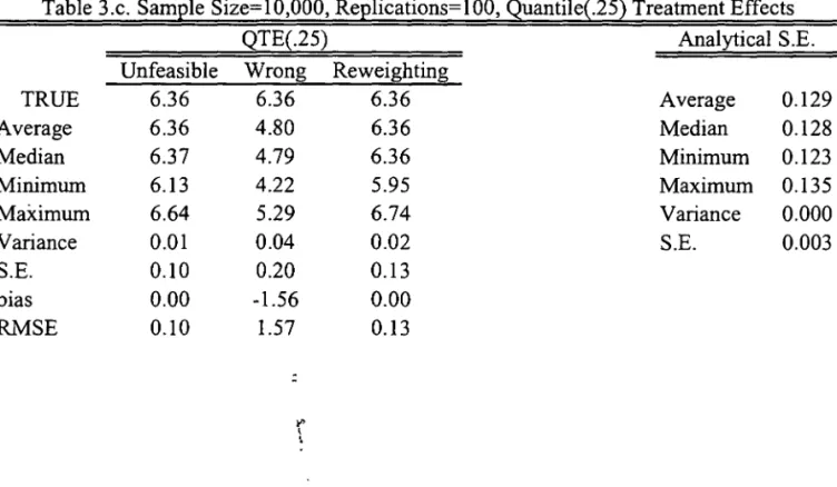
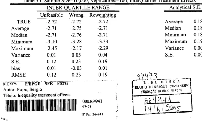
Results can be found in Tables 1-4. Each one of Tables 1-3 reports estimates of different

treatment effect parametersj they differ in the sample size considered. In each of those tables,

we report average, variance, quantile (lower quartile, median, upper quartile) and inter-quartile

range treatment effects. Analytical standard errors are also computed and they appear on the

right side of each of those tables.14

The results indicate that the reweighting estimator performs well according to the MSE

criteria. Also, looking separately at bias and variance terms, it is dear that the bias vanishes

relatively fast as the sample increases for all of the parameters being estimated by the

reweight-ing method, the same not occurrreweight-ing with the "wrong" estimator, which is basically an estimator

of li _{(FY (l)jT=l) -} li (FY(O)jT=O)' Analytical standard errors tend to be (either looking at the

average or at the median) dose to the bootstrapped standard errors for all sample sizes and all

14The polynomial order for both the propensity-score estimation and the asymptotic variance estimation can

be determined by cross-validation. In order to simplify our computations we fixed the propensity-score to have

parameters. This indicates that bootstrapping may be a good alternative to analytical standard

errors estimation.

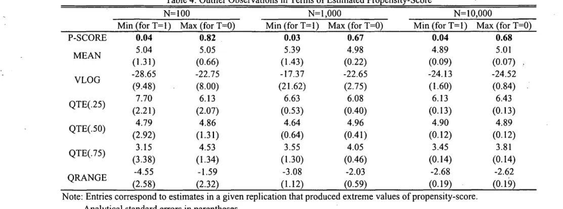
There is one important point that can be seen clearly through the analytical standard

errors formulae and which reveals itself to be relevant in the Monte Carlo exercise. In samples

with "weak" common support, that is, when the estimated propensity-score may assume values

"close" to either O or 1, the standard errors will refiect that situation. From Equation 12 we can

see for the treated, a low propensity score will increase standard errors, the same happening with

a high propensity-score for the untreated. In Table 4 we report the minimum and maximum

values among all samples and replications for a given sample size respectively for the treated

and the control units. As expected, higher biases and larger standard errors tend to occur when

there is weak common support problems.

This last fact allows us to draw an analogy with the famous discussion of multicollinearity in

Goldberger's textbook, a discussion also known by introducing the "micronumerosity" problem

in the literature.15 Samples with poor overlapping in terms of covariates among treated and controls will produce imprecise and uninformative estimates of treatment effects, the same

happening with multicollinear regressors and regression coefficient estimates. Trimming with

respect to distribution of the propensity-score has the same fiavour of dropping a regressor that

is highly correlated with some other one in order to "solve" the multicollinearity problem: It

leads to an estimate of another parameter, not the one we were initially interested in. The

assertion that "more data will be of no help if it is more of the same" is aIs o true here:

More data will be of no help if we still have no or little intersection in the supports of the

covariates empirical distributions given treatment assignment. Finally, putting into brackets

our comments so we can draw the analogy more precisely, we cite Goldberger's first remark

about multicollinearity on page 251: "Researchers should not be concerned with whether or

not "there really is collinearity" [no-overlapping in the support in our case]. They may well be

concerned with whether the variances of the coefficient estimates are too large - for whatever

reason - to provide useful estimates of the regression coefficients [treatment effects in our case]."

We may conclude then that the claim that reweighting method is of little importance because

it does not solve the common support problem sounds similar to say that OLS is of little

importance because it is not robust to multicollinearity.

15See Goldberger (1991), chapter 23.

20

FUNDAÇÃO GE'fULlO VARGÀS BIBLIOTECA MARIO HENRIQUE SlMONSEN

,--6

Conclusion

In this paper we proposed estimators for the effects of a treatment on some inequality measures.

This was achieved by first estimating, through a reweighing method, the inequality measures of

the potential outcomes, and then taking the difference between those estimates. This

estima-tion strategy is useful for policy-making purposes when the individual decision to participate

into the social program (the treatment) depends on observable characteristics. If the

identifica-tion restricidentifica-tions hold, then the reweighing method allows identify the distribuidentifica-tion of potential

outcomes and, therefore, many of their inequality parameters.

We showed that the inequality treatment effect estimators are root-N consistent and

as-ymptotically normal. We also calculated the semiparametric efficiency bounds and proved that

the proposed estimators achieve them.

Finally, we performed a series of Monte Carlo exercises. The reweighting estimator

per-formed well in terms of the MSE criteria. It aIs o seemed that finite sample bias vanishes fast as

the sample size increases. Analytical standard errors behaved similarly to bootstrapping ones,

revealing that bootstrap may be a valid alterna tive. However, the interpretation gain from the

analytical expression is important: if the covariates in the treated just "weakly" share the same

support of distribution with covariates in the control group, then the standard errors of the

reweighting estimator will reflect the fact that the comparisons across groups will be poor and

REFERENCES

ABADIE, A., J. ANGRIST, AND G. IMBENS, (2002), "Instrumental Variables Estimation of

Quantile Treatment Effects," Econometrica, 70, 91-117.

BICKEL, P., C. KLASSEN, Y. RITOV, AND J. WELLNER, (1993), Efficient and Adaptive

Estimation for Semiparametric Models. New York, Springer-Verlag.

BITLER, M., J. GELBACH, AND H. HOYNES, (2004), "What Mean Impacts MissL

Distribu-tional Effects of Welfare Reform Experiments," preprint.

CHEN, X., H. HONG, AND A. TAROZZI, (2004), "Semiparametric Efficiency in GMM Models

of Nonclassical Measurement Errors, Missing Data and Treatment Effects," preprint.

COWELL, F., (2000), "Measurement of Inequality," in Handbook of Income Distribution, ed.

by A. Atkinson, and F. Bourguignon, North Holland, Amsterdam.

COWELL, F., (2003), "Theil, Inequality and the Structure of Income Distribution,"

Distribu-tional Analysis Discussion Paper, STICERD, L SE, No. 67.

DINARDO, J., N. FORTIN, AND T. LEMIEUX, (1996), "Labor Market Institutions and the

Distribution of Wages, 1973-1992: A Semiparametric Approach," Econometrica, 64,

1001-1044.

FIRPO, S. (2004), "Efficient Semiparametric Estimation of Quantile Treatment Effects," UBC

Deparlment of Economics Discussion Paper, No. 04-01.

GOLDBERGER, A. (1991), A Course in Econometrics. Cambridge, Harvard University Press.

HAHN, J., (1998), "On the Role of the Propensity Score in Efficient Semiparametric Estimation

of Average Treatment Effects," Econometrica, 66, 315-331.

HECKMAN,J., AND B. HONORÉ (1990), "The Empirical Content of the Roy Model,"

Econo-metrica, 58, 1121-1149.

HECKMAN, J., H. ICHIMURA, AND P. TODD, (1997), "MatchingasanEconometricEvaluation

Estimator," Review of Economic Studies, 65(2), 261-294.

HECKMAN, J., H. ICHIMURA, J. SMITH, AND P. TODD, (1998), "Characterizing Selection

Bias Using Experimental Data," Econometrica, 66, 1017-1098.

HECKMAN, J., J. SMITH, AND N. CLEMENTS, (1997), "Making the Most out of Programme

Evaluations and Social Experiments Accounting for Heterogeneity in Programme

Im-pacts," Review of Economic Studies, 64(4), 487-535.

HIRANO, K., G. IMBENs, AND G. RIDDER, (2003), "Efficient Estimation of Average

Treat-ment Effects Using the Estimated Propensity Score," Econometrica, 71, 1161-1189.

HUBER, P. (1981), Robust Statistics. New York, John Wiley & Sons.

IMBENS, G., AND D. RUBIN, (1997), "Estimating Outcome Distributions for Compliers in

Instrumental Variable Models," Review of Economic Studies, October, 555-574.

MANSKI, C. (1997), "The Mixing Problem in Programme Evaluation," Review of Economic

Studies, October, 537-554.

NEWEY, W., (1990), "Semiparametric Efficiency Bounds," Journal of Applied Econometrics,

5, 99-135.

NEWEY, W., (1994), "The Asymptotic Variance of Semiparametric Estimators,"

Economet-rica, 62, 1349-1382.

NEWEY, W., (1995), "Convergence Rates for Series Estimators," in Advances in Econometrics

and Qualitative Economics: Essays in Honor of C.R. Rao, G. Maddala, P.C. Phillips, and

T.N. Srinivasan, eds., Cambridge US, Basil-Blackwell.

NEWEY, W., (1997), "Convergence Rates and Asymptotic Normality for Series Estimators,"

Journal of Econometrics, 79, 147-168.

Roy, A., (1951), "Some Thoughts on the Distribution of Earnings," Oxford Economic Papers,

3(2), 135-146.

ROSENBAUM, P., AND D. RUBIN, (1983), "The Central Role of the Propensity Score In

ROSENBAUM, P., AND D. RUBIN, (1984), "Reducing Bias in Observational Studies Using

Sub-classification on the Propensity Score," Journal 01 the American Statistical Association,

79, 516-574.

RUBIN, D., (1977), "Assignment to Treatment Group on the Basis of a Covariate," Journal

01 Educational Statistics, 2(1), 1-26.

VAN DER VAART, A. (1998), Asymptotic Statistics. Cambridge, Cambridge University Press.

....--r--~---

--APPENDIX: Proofs

Proof of Lemma 1:

Fix y, where Y E Supp (Y (1)), the support of Y (1). Let us work with FY(l)(Y) as the other

c.dJ.'s follow by simple analogy. FY(l)(Y) = Pr[Y(I) :S y} = lE[Pr[Y(I) :S Y

I

X]] = lE[Pr[Y(I) :S

Y

I

X, T = lJJ = lE[Pr[Y:S yl X, T = lJJ = lE[lE[T lI{Y :S y}1 X, T = 1]]

=lE[p(3c) lE[TlI{Y:SY}IXJ]

=lE[P(~)

lI{Y:Sy}].

The first equality follows from the definition of the c.dJ.. The second is an application

of the law of iterated expectations. The third equality follows from the ignorability

assump-tion (Assumpassump-tion 1). The fourth results from the definiassump-tion of Y = TY(I)

+

(1 - T)Y(O).

The fifth equality comes from lE[lI{A}J = Pr[AJ (where A is some event) and from the fact

that the expectation is conditional on T = 1. The sixth is a consequence from lEr Z

I

XJ =

p(X)lE[Z

I

X, T = lJ

+

(1 - p(X))lE[Z

I

X, T = O], where Z is some random variable with finite

variance and fram the common support assumption (Assumption 2). Finally, the last equality is

a backward application of the law of iterated expectations. Analogous results for Fy(o) (y) and

FY(O)IT=l (y) could have been derived following essentially the same steps as above. The result

for FY(l)IT=l(Y) could have been easily proved but with not using the ignorability assumption

as that c.dJ. is identifiable from data on Y for T = 1. •

Proof of Corollary 1:

Let us define Yy:T/p(X) and Yy:(l-T}/(l-p(X)) the reweighted distribution functions of Y

using Tjp(X) and (1 - T) j (1-p(X)) as weights. From Lemma 1, Yy:T/p(X) = FY(l) and

Yy:(l-T)/(l-P(X)) = Fy(o). From Assumption 3, as FY(l) = F;:T/p(X), we have that 11 (FY(1)) =

( nW:T/P(X)). d F - nW:(l-T)/(l-p(X)) h th t (F ) _ (nW:(l-T)/(l-P(X)))

11 ry ,an as Y(O) - ry ,we ave a 11 Y(O) - 11 ry .

Therefore, ~v is identified from data on (Y, T, X). The same holds by analogy to ~vIT=l. •

Proof of Lemma 2:

See Hirano, 1mbens and Ridder (2003), Lemmas 1 and 2 . •

Proof of Theorem 1: [Part (i) J

Let us again concentrate on VY(l)' since extensions to other functionals estimates follow

Under Assumption 6, the unfeasible estimator of YY(1) is asymptotically linear: y

(F{:t(1))

-y (FY(l)) -

k

L:I:l 'l/Jv

(li

(1) ; Ov,Y(l)) = op(Ij..JN). Now consider that we have a new

sam-pling scheme, based on ignorability. Thus, we just replace

F{:t(l) ,

the empirical distribution under random sampling or full observability of Y (1), by

FY(l) ,

the empirical distribution under ignorability. We have that:

(A-I)

Now, define

Thus Equation A-I can be rewritten as:

And we need to show that ~N

=

op(Ij.JN). In order to show that, rewrite ~N as:

~N

=

2.

~

(Ti' 'l/Jv

~li;

Ov,Y(l)) _ Ti' 'l/Jv

(li;

Ov,Y(l))

+

Ti' 'l/Jv

(li;

Ov,Y(l)) (P(X

i) _ p(Xi)))

N

t-:

p(Xi) p(Xi) p2(Xi)

(A-2)

-

~

t

(Ti .

"'"p~~

~~;.Y(l})

(P(Xi) - p( Xi)))

+

IE

[lEI"'"

(Y;

9";~i

I

X, T =

11

(p( X) - p( X))]

(A-3)

-]E []E['l/Jv (Y; Ov,Y(l))

I

X, T = 1] (p(X) _ P(X))]-

2.

t

5(X_i, u) Ti - PK(Xi)

p(X) N i=l VPK(Xi)(I - PK(Xi))

(A-4)

(A-5)

(A-6)

"

where:

8(Xi, u)

~

-E

[E[,pv

(y;

IIv~~i

[X, T

~

1 [ L' (HK (X)';r )HK(X)'

1

f;-l.j

L' (HK(Xi)'7r K )HK (Xi)

Ó K(Xi, u)

~

-E

[E[,pV

(y;

IIv~~i

[X, T

~

1

J L' (HK(X)' 7r K)H K( X)'

1

E,/.j

L'( HK(Xi)'7r K )HK(Xi)

Vp(Xi)(l - p(Xi))

Ó(Xi, u)

=

-1E[1/!//

(Y; O//,Y(l)) IXi, T

=

1]

p(X

i)

N

f:

=

~

L

HK (Xi)HK (XdL'(HK (Xi)'ir)

i=l

and

Hirano, Imbens and Ridder (2003) have computed their first step in the exact same way we do.

Also, in their Theorem 1 they have a remainder term to bound very similar to ~N' The main

difference is that instead of

1/!//

(Y; O//,Y(l)) they have Y, where

1E[y

2] is assumed to be finite

and have continuously differentiable conditional expectation given X and T = 1. We have made a similar assumption, but to the infiuence function

1/!//

(Y; O//,Y(l)) ' by imposing Assumption 5. It is then possible to bound ~N using exactly the same arguments they used. Firpo (2004)

has shown how to draw the analogy between HIR's proof for the average treatment effects and

the quantile treatment effects. In order to avoid repetition of the same argument, we refer the

reader to their proofs (Lemma 3 in Firpo (2004), Theorem 1 in Hirano, Imbens and Ridder

(2003)). A complete proof is, however, available upon request. Therefore, replacing Y -

f3

by

1/!//

(Y; O//,Y(l)) in HIR, we can conclude that ~N

=

op(ljVN).

Extending the result to vY(O) is trivial. Thus, making use of the fact that 1:1// is just the

differ-ence between LlY(l) and Lly(O) we can conclude that:

VN

(Li// -

1:1//) =

JN

L:f:l

1/!

~

(Yi,

Xi, Ti; 0//)

+op(l)

~

N

(O,

O'~J

.•

Proof of Theorem 1: [Part (ii)]

We have now to show that

O't

is indeed the semiparametric efficiency bound of 1:1//. This

proof is an extension to this general parameter case of the proofs by Hahn (1998) and Hirano,

Imbens and Ridder (2003) for the mean case and by Firpo (2004) for the quantile case. These

references use the machinery presented by Bickel, Klassen, Ritov, and Wellner (1993), Newey

-By the same reason as before, we concentrate attention to v

(F

_Y

(1))

and its semiparametric efficiency bound. An extension to v (Fy(o)) and therefore to the treatment effect ~y will follow

byanalogy.

Let us divide the problem into two parts. In the first part we discuss the model in which

there is fuIl observability of Y (1); in the second part we discuss what happens when we have

ignorability instead.

Under fuIl observability the tangent space is characterized by S[ULL, which has been defined

previously. Any efficient estimator of parameters of this model wiIl have to have its asymptotic

infiuence function belonging to S[ULL. By Assumption 7 'l{;y (y; OY(l))

=

cPy

(y, t, x; OY(l)) E

S[U LL. As 'l{;y (Y; OY(l)) does not depend on (t, x) we conc1ude that it has to satisfy O

=

1E['l{;y (Y (1); OY(l))]' Also, because v

(F~(1))

is asymptotically linear and regular by

Assump-tion 6, then by BKRW's ProposiAssump-tion 3.3.1 v is pathwise differentiable, that is, for any regular

parametric sub-model indexed by a finite dimensional vector iJ, we have:

v (FY(l) (iJ)) - v (FY(l))

=

J

'l{;y (y; OY(1)) . dFY(l) (y; iJ) -

J

'l{;y (y; OY(l)) . dFY(l) (y)

+

o (11iJ - iJoII) .

J

'l{;y (y; OY(1)) . dFY(l) (y; iJ)

+

o (IIiJ - iJo 11)

where we have used the following notational normalization: FY(l) (iJo) = FY(l)' and where

iJo is the true population parameter. Thus, the derivative of v (FY(1) (iJ)) with respect to iJ

evaluated at iJo has to be equal to:

âv(FY(l) (iJo))

J

OiJ = 'l{;y (y; OY(l)) . Sl(Y) . dFY(l) (y)

where Sl(Y) is the score function of the distribution FY(l) evaluated at the true parameter

model.

Under ignorability, start defining the densities, with respect to some cr-finite measure, of

(Y(l), T, X) and of the observed data (Y, T, X). Under Assumption 1, both densities represent

the same statistical model and are, therefore, equivalent. These densities can be written as

f Y(l),T,X(y,t, x)

=

(JY(l)lx(ylx) .p(x))t. fx(x) and f Y,T,X(y,t, x)

=

(JYIX,T=l(ylx) .p(x))t.

fx(x). Working with the density of observed data, consider the regular parametric sub-model

indexed by iJ:

fY,T,X(y, t, x

I

iJ) = (JYIX,T=l(Y

I

x; iJ) . p(x

I

iJ))t . fx(x

I

iJ),

28

By a normalization argument, let fy,T,X(Y, t, x) = fy,T,X(Y, t, x 1190). The score of a parametric sub-mo deI indexed by 19 is given by:

s(y, t, x 1 '19) = t· Sl(Y 1 x; '19)

+

p(xtl '19) . p'(x 119)

+

sx(x 1 '19)

where, for

SI

(y 1 x; '19) =

:8

log fYIX,T=l (y 1 x; 19); p'(x 119) = :eP(x 119); and Sx(x 119) =

:8

log f(x 119).

Again we normalize: s(y, t, x) = s(y, t,

xl

'190). In order to find the efficient influence func-tions of the parameters of interest, 1/ (FY(l») we need first to define the tangent space of this statistical mode!. This will be the set S of all possible score functions, and it is de-fined as: S

=

{S : IR x {O, I} x X - t IR 1 S(y, t, x)

=

t· Sl(Y 1 x)

+

+a(x) . t

+

sx(x); and

lE[Sl(Y 1 X) 1 X = x, T = 1] = lE[sx(X)] = 0, Vx and where a(x) is square-integrable function of

x}. N ext note that 1/ is still pathwise differentiable under the ignorability model, as 1/ (FY(l) ) is a regular asymptotically linear estimator of 1/ (FY(l») as consequence of part (i) of Theorem

1. Thus 1/ (FY(l) ('19)) can be written as:

1/ (FY(l) (19)) - 1/ (FY(l»)

/

4J~

(y;

OY(l») . dFY(l) (y; 19) - /

<p~

(y; OY(l») . dFY(l) (y)

+

0(1119 - 19011)

= / /

'Ij;~

(y, t, x; OY(l») . fYIX,T=l (y 1 x; '19) . f(x 119) . dy . dx

+

o (1119 - 19011) where <p~ (y; OY(l») is a bounded linear functional of FY(l) such that

Thus, the derivative of 1/ (FY(l) (19)) with respect to '19 evaluated at 190 has to be equal to:

/ /

'Ij;~

(y, t, x; OY(l») . Sl(y 1 x) . fYIX,T=l (y 1 x) . f(x) . dy· dx

+ / (/

'Ij;~

(y, t, x; OY(l») . fYIX,T=l(y 1 x) . dY) . sx(x) . f(x) . dx.

We know that 'Ij;~ (y, t, x; OY(l») will be the efficient influence function of 1/ (FY(l») if 'Ij;~ (y, t, x; OY(l») E S. By the uniqueness of the efficient influence function, <p~ (y; OY(l») = 'Ij;// (y; OY(l»)' and therefore, a natural candidate for 'Ij;~ (y, t, x; OY(l») is:

'Ij;~

(y, t, x; OY(l») = p !x)

.('Ij;//

(y; O//,Y(l») -lE

['Ij;//

(Y; O//,Y(l») 1 x, T = l])+lE

['Ij;//

(Y; O//,Y(l») 1 x, T = 1J '