Topographic control of snowpack distribution in a small catchment in the central Spanish Pyrenees: intra- and inter-annual persistence

(1)

TCD

8, 1937–1972, 2014

Topographic control of snowpack

distribution

J. Revuelto et al.

Title Page

Abstract Introduction

Conclusions References

Tables Figures

◭ ◮

Back Close

Full Screen / Esc

Printer-friendly Version Interactive Discussion

Discussion

P

a

per

|

D

iscussion

P

a

per

|

Discussion

P

a

per

|

Discuss

ion

P

a

per

|

The Cryosphere Discuss., 8, 1937–1972, 2014 www.the-cryosphere-discuss.net/8/1937/2014/ doi:10.5194/tcd-8-1937-2014

Open Access

The Cryosphere

Discussions

This discussion paper is/has been under review for the journal The Cryosphere (TC). Please refer to the corresponding final paper in TC if available.

Topographic control of snowpack

distribution in a small catchment in the

central Spanish Pyrenees: intra- and

inter-annual persistence

J. Revuelto, J. I. López-Moreno, C. Azorin-Molina, and S. M. Vicente-Serrano

Instituto Pirenaico de Ecología, Consejo Superior de Investigaciones Científicas (IPE-CSIC) Departamento de Procesos Geoambientales y Cambio Global, Campus de Aula Dei, P.O. Box 13034, 50059, Zaragoza, Spain

Received: 3 March 2014 – Accepted: 2 April 2014 – Published: 15 April 2014 Correspondence to: J. Revuelto ([email protected])

(2)

TCD

8, 1937–1972, 2014

distribution

J. Revuelto et al.

Title Page

Tables Figures

◭ ◮

Back Close

Full Screen / Esc

Discussion

P

a

per

|

D

iscussion

P

a

per

|

Discussion

P

a

per

|

Discuss

ion

P

a

per

Abstract

In this study we analyzed the relations between terrain characteristics and snow depth distribution in a small alpine catchment located in the central Spanish Pyrenees. Twelve field campaigns were conducted during 2012 and 2013, which were years character-ized by very different climatic conditions. Snow depth was measured using a long range

5

terrestrial laser scanner and analyses were performed at a spatial resolution of 5 m. Pearson’s r _{correlation, multiple linear regressions and binary regression trees were}

used to analyze the influence of topography on the snow depth distribution. The analy-ses were used to identify the topographic variables that better explain the snow distri-bution in this catchment, and to assess whether their contridistri-butions were variable over

10

intra- and inter-annual time scales. The topographic position index, which has rarely been used in these types of studies, most accurately explained the distribution of snow accumulation. Other variables affecting the snow depth distribution included the maxi-mum upwind slope, elevation, and northing (or potential incoming solar radiation). The models developed to predict snow distribution in the basin for each of the 12 survey

15

days were similar in terms of the most explanatory variables. However, the variance ex-plained by the overall model and by each topographic variable, especially those making a lesser contribution, differed markedly between a year in which snow was abundant (2013) and a year when snow was scarce (2012), and also differed between surveys in which snow accumulation or melting conditions dominated in the preceding days. The

20

(3)

TCD

8, 1937–1972, 2014

distribution

J. Revuelto et al.

Title Page

Tables Figures

◭ ◮

Back Close

Full Screen / Esc

Discussion

P

a

per

|

D

iscussion

P

a

per

|

Discussion

P

a

per

|

Discuss

ion

P

a

per

|

1 Introduction

Assessing the snow distribution in mountain areas is important because of the num-ber of processes in which snow plays a major role, including erosion rates (Pomeroy and Gray, 1995), plant survival (Keller et al., 2000; Wipf et al., 2009), soil temperature and moisture (Groffman et al., 2001), and the hydrological response of mountain rivers

5

(Bales and Harrington, 1995; Barnett et al., 2005; Liston, 1999; Pomeroy et al., 2004). As mountain areas are highly sensitivity to global change (Beniston, 2003), snow accu-mulation and melting processes are likely to be subject to marked changes in coming decades, affecting all processes influenced by the presence of snow (Caballero et al., 2007; López-Moreno et al., 2011, 2012b; Steger et al., 2012). For these reasons, much

10

effort has been devoted to understanding the main factors that control the spatial and temporal dynamics of snow (Egli et al., 2012; López-Moreno et al., 2010; ; Mott et al., 2010; Schirmer et al., 2011).

One of the main difficulties in snow studies is obtaining reliable information of the variables that describe snow distribution, including snow depth (SD), snow water

equiv-15

alent (SWE) and snow covered area (SCA). Manual measurements have traditionally been used to provide information on the distribution of snowpack, with different sam-pling strategies having been applied at various spatial scales (Jost et al., 2007; López-Moreno et al., 2012a; Watson et al., 2006). However, manual sampling is not feasible for large areas because of the time involved, especially when SWE measurements are

20

also acquired. In the last decade the use of airborne laser scanners (ALS) (Deems et al., 2006) and terrestrial laser scanners (TLS) (Prokop, 2008), both of which are based on LiDAR (laser imaging detection and ranging) technology, have provided for major advances in obtaining data on the SD distribution at unprecedented spatial res-olutions. These developments have enabled studies of several factors that in the past

25

(4)

TCD

8, 1937–1972, 2014

distribution

J. Revuelto et al.

Title Page

Tables Figures

◭ ◮

Back Close

Full Screen / Esc

Discussion

P

a

per

|

D

iscussion

P

a

per

|

Discussion

P

a

per

|

Discuss

ion

P

a

per

2011; Scipión et al., 2013), and snow transport processes (Mott et al., 2010). In ad-dition, the high density measurements provided by LiDAR technologies are a valuable resource for detailed investigation of the linkage between snow distribution and topog-raphy. In the past, this linkage has mostly been studied using manual measurements, and hence with generally limited spatial and temporal resolution (López-Moreno et al.,

5

2010).

Previous studies have highlighted the marked control of topography on snow distri-bution in mountain areas (Anderton et al., 2004; Erickson et al., 2005), and the impor-tance of vegetation and wind exposure (Erxleben et al., 2002; Trujillo et al., 2007). The most commonly used approach has been to develop digital elevation models (DEM)

10

that describe the spatial distribution of elevation, from which other terrain variables are derived including slope, terrain aspect, curvature, wind exposure or sheltering, and potential solar radiation. This enables to analyze the linear or non-linear relation of these variables to punctual SD or SWE values to be established (Grünewald et al., 2010; Schirmer et al., 2011). Various statistical methods have been applied for this

15

purpose, including linear regression models (Fassnacht et al., 2003; Hosang and Det-twiler, 1991), generalized additive models (GAM) (López-Moreno and Nogués-Bravo, 2005), and binary regression trees (BRT) (Breiman, 1984) which have been widely ap-plied in a diversity of regions (Elder et al., 1991; Erxleben et al., 2002; McCreight et al., 2012).

20

The extent to which topographic variables explain snow distribution can change dur-ing the snow season; the variability of terrain characteristics can drive processes re-lated to the spatial variability of snow accumulation (snow blowing, terrain curvature) (Lehning et al., 2008), or affect the energetic exchange between terrain and the snow-pack (temperature, incoming solar radiation), so the importance of topographic

vari-25

(5)

TCD

8, 1937–1972, 2014

distribution

J. Revuelto et al.

Title Page

Tables Figures

◭ ◮

Back Close

Full Screen / Esc

Discussion

P

a

per

|

D

iscussion

P

a

per

|

Discussion

P

a

per

|

Discuss

ion

P

a

per

|

studies have assessed whether the influence of topography is constant among different years; e.g. the similarities observed at the end of the accumulation season (Schirmer and Lehning, 2011; Schirmer et al., 2011), or the consistent fractal dimensions in two analyzed years (Deems et al., 2008); in both cases there was a relation with the domi-nant wind direction, which highlights the predictive ability of topographic variables.

5

The main focus of this study was to assess the influence of topography on the spatial distribution of snowpack and its evolution over time. The high temporal and spatial den-sity of the dataset collected during the study enabled analysis of the main topographic factors controlling snow distribution, and assessment of whether topographic control of the snowpack varied during the snow season and between years having very

contrast-10

ing climatic conditions. For this purpose, we conducted 12 surveys over 2012 (6) and 2013 (6) in a small mountain catchment representing a typical subalpine environment in the central Spanish Pyrenees, and obtained high resolution SD measurements using LIDAR technology using a TLS.

2 Study area and snow and climatic conditions

15

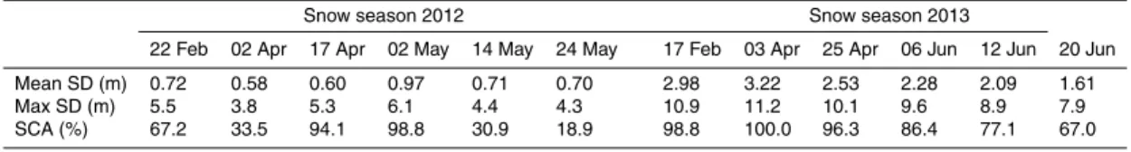
The Izas experimental catchment (42◦44′N, 0◦25′W) is located in the central Spanish Pyrenees (Fig. 1). The catchment is on the southern side of the Pyrenees, close to the main divide (Spain–France border), in the headwaters of the Gallego River valley, and ranges in elevation from 2000 to 2300 m a.s.l. The catchment is predominantly east-facing, with some areas facing north or south, and has a mean slope of 16◦. There are

20

no trees in the study area, and the basin is mostly covered by subalpine grasslands dominated by Festuca eskia and Nardus stricta, with rocky outcrops in the steeper areas; flat, concave and convex areas occur in the basin.

The climatic conditions are influenced by the proximity of the Atlantic Ocean, with the winters being humid compared with zones of the Pyrenees more influenced by

25

(6)

temper-TCD

8, 1937–1972, 2014

distribution

J. Revuelto et al.

Title Page

Tables Figures

◭ ◮

Back Close

Full Screen / Esc

Discussion

P

a

per

|

D

iscussion

P

a

per

|

Discussion

P

a

per

|

Discuss

ion

P

a

per

ature is 3◦C, and the mean daily temperature is<₀◦_{C for an average of 130 days each}

year (del Barrio et al., 1997). Snow covers a high percentage of the catchment from November to the end of May.

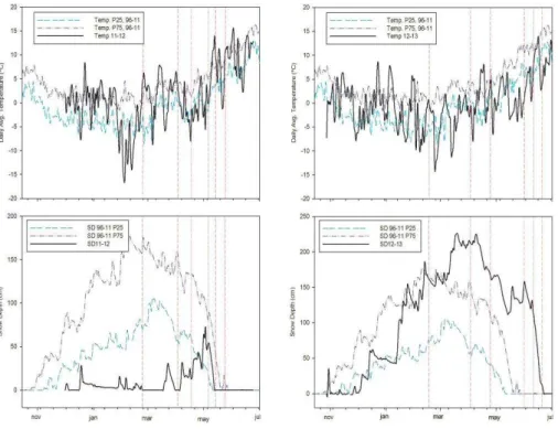
The two years analyzed in the study represent climatic extremes during recent decades. Severe drought occurred during 2012, leading to snow accumulation well

5

below the long-term average. The thickness of the snowpack during winter in this year was less than the 25th percentile of the available historical data series (1996–2011) (Fig. 2). Only at the end of spring did late snowfall events increase the amount of snow, but this rapidly melted. The opposite occurred in 2013, which was a year in which the deepest snowpack and the longest snow season of recent decades were recorded.

10

Winter and spring in 2013 were extremely humid, with temperatures mostly between the 25th and 75th percentiles of the historical series. Snow depth accumulation was very high between February and June (exceeding the 75th percentile); in some areas of the basin it lasted until late July, which is one month longer than in most of the preceding years for which records are available.

15

3 Data and methods

3.1 Snow depth measurements

During the study period high resolution SD maps were generated using a long range TLS (Riegl LPM-321), which enables safe acquisition of SD information with short ac-quisition times from remote areas, compared with measurements obtained manually.

20

This technique has been extensively tested (Prokop et al., 2008; Revuelto et al., 2014; Schaffhauser et al., 2008), and systematically applied to the study of snow distribution in mountain terrain (Grünewald et al., 2010; Schirmer and Lehning, 2011; Schirmer et al., 2011). In a previous study the mean absolute error in the most distant areas of the catchment was less than 10 cm (Revuelto et al., 2014), which is consistent with

25

(7)

TCD

8, 1937–1972, 2014

distribution

J. Revuelto et al.

Title Page

Tables Figures

◭ ◮

Back Close

Full Screen / Esc

Discussion

P

a

per

|

D

iscussion

P

a

per

|

Discussion

P

a

per

|

Discuss

ion

P

a

per

|

TLS provides high resolution three dimensional information on the terrain. Neverthe-less, error sources need to be considered because they can have large effects on the measurements. To reduce the influences of TLS instability (which leads to misalign-ment with reference points) and atmospheric change, a well-defined protocol must be applied. The protocol applied in this study for generating high resolution SD maps with

5

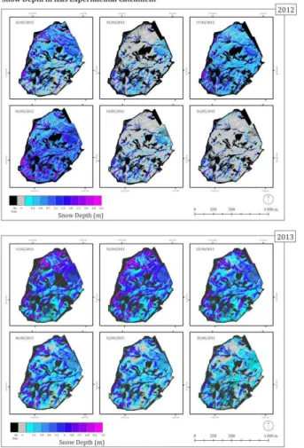
a 1 m cell size was described by Revuelto et al. (2014). The methodology was based on differences between DEMs obtained with snow coverage in the study area and a DEM taken at 18 July 2012, when the catchment had no snow cover. Twelve snow depth maps at a spatial resolution of 5 m were generated for the 2012 and 2013 snow sea-sons (Fig. 3). In each year three surveys were undertaken from February to April during

10

the snow accumulation period (2012: 22 February, 2 April, 17 April; 2013: 17 February, 3 April, 25 April), and three were undertaken from May to June in the snowmelt period (2012: 2, 14 and 24 May; 2013: 6, 12 and 20 June). The average SD and SCA, and the maximum SD are shown in Table 1.

3.2 Digital elevation model and topographic variables

15

From the two scan stations (Revuelto et al., 2014) located in the study area (Fig. 1), 86 % of the total area of the catchment was surveyed using TLS at an initial spatial resolution of 1 m grid size. Some of the predictor variables cannot be calculated where data gaps occur in the DEM (e.g. the topographic position index), and others require a DEM with a greater surface than the area scanned during the study (e.g. to calculate

20

the potential solar radiation, including the shadow e_ffect from surrounding topography, or to calculate the maximum upwind slope parameter). Thus, a DEM having a 5 m grid-size, available from the Geographical National Institute of Spain (Instituto Geográfico Nacional, www.ign.es), was combined with the snow-free DEM obtained using the TLS resampled from 1 m to 5 m resolution (the empty raster of the Geographical National

25

(8)

TCD

8, 1937–1972, 2014

distribution

J. Revuelto et al.

Title Page

Tables Figures

◭ ◮

Back Close

Full Screen / Esc

Discussion

P

a

per

|

D

iscussion

P

a

per

|

Discussion

P

a

per

|

Discuss

ion

P

a

per

To characterize the terrain characteristics, eight variables were derived from the final DEM, including: (i) elevation (Elevation), (ii) slope (Slope), (iii) curvature (Curvature), (iv) potential incoming solar radiation under clear sky conditions (Radiation), (v) easting exposure (Easting), (vi) northing exposure (Northing), (vii) the topographic position index (TPI) and (viii) maximum upwind slope (Sx).

5

Elevationwas obtained directly from the DEM, while the other variables were calcu-lated using ArcGIS10.1 software. This calculatesSlopeas the maximum rate of change in value from a specific cell to that of its neighbors, and Curvature is determined from the second derivative of the fitted surface to the DEM. Radiation was obtained us-ing the algorithm of Fu and Rich (2002) and reported in watts hour per square meter

10

based on the average conditions for the 15 day period prior to each snow survey. This measure provided the relative difference in the extraterrestrial incoming solar radiation among areas of the catchment for a given period under given topographical conditions (Fassnacht et al., 2013). Easting and Northing exposure were calculated directly as the sine and cosine of the angle between direction north and the maximum slope line

15

of the terrain, respectively. It provided information on the east (positive)/west (negative) exposure and the north (positive)/south (negative) exposure.

TheTPI provided information on the relative position of a cell in relation to the sur-rounding terrain at a specific spatial scale. Thus, this index compared the elevation of each cell with the average cell elevation at various radial distances (Weiss, 2001). For

20

each pixel theTPIwas calculated for 10, 15, 25, 50, 75, 100, 125, 150 and 200 m radial distances.

For specific wind directions, the maximum upwind slope parameter (Sx; Winstral et al., 2002) provided information on the exposure or sheltering of individual cells at various distances, resulting from the topography. Rather than considering the

contribu-25

(9)

TCD

8, 1937–1972, 2014

distribution

J. Revuelto et al.

Title Page

Tables Figures

◭ ◮

Back Close

Full Screen / Esc

Discussion

P

a

per

|

D

iscussion

P

a

per

|

Discussion

P

a

per

|

Discuss

ion

P

a

per

|

135◦for southeast (SE), 180◦for south (S), 225◦for southwest (SW), 270◦for west (W), and 315◦ for northwest (NW). For Sx the searching distances (Winstral et al., 2002) considered were 100, 200, 300 and 500 m. These distances were selected to enable assessment of the range at whichSx exhibited greatest control on SD dynamics, as has occurred in previous studies (Schirmer et al., 2011; Winstral et al., 2002).

5

3.3 Statistical analysis

The 12 SD maps at 5 m spatial resolution were related to each of the topographic variables considered (including the 40Sx combinations, and the 9 distances forTPI). The large number of cells for which snow depth data were available enabled robust correlations between topography and snow distribution to be obtained, and provided

10

a very large dataset for training and validation of the SD distribution models.

Pearson’sr _coe_ffi_{cients were obtained between SD and each topographic variable.}

Given the large amount of data for each sample, the degrees of freedom for the cor-relation analyses were very high. For this reason we followed a Monte Carlo proce-dure, in which 1000 random samples of 100 SD cases were extracted from the entire

15

dataset and correlated with topographic variables. A threshold 95 % confidence interval (α <_{0.05) was used to assess the significance of correlations (}r₌_±_{0.197, based on}

100 cases) (Zar, 1984). The spatial scales ofSx (200 m) andTPI (25 m), for which SD showed a higher correlation, were selected for further analysis.

To assess the explanatory capacity when all topographic variables were considered

20

simultaneously, two statistical models were used: (1) multiple linear regressions (MLRs) and (2) binary regression trees (BRTs). A wide variety of regression analyses for inter-pretation of much more complex spatial data are available with greater capacity than MLRs and BRTs to deal with spatial autocorrelation issues and the non-linear nature of the relationship between predictors and the response variable (Beale et al., 2010).

25

(10)

TCD

8, 1937–1972, 2014

distribution

J. Revuelto et al.

Title Page

Tables Figures

◭ ◮

Back Close

Full Screen / Esc

Discussion

P

a

per

|

D

iscussion

P

a

per

|

Discussion

P

a

per

|

Discuss

ion

P

a

per

the weight of each independent variable within the model, which was the main objective of this research, rather than deriving models with maximum predictive capacity.

1. Multiple linear regression estimates the linear influence of topographic variables on SD. Despite its simplicity and the rather limited capability under nonlinear ditions (López-Moreno et al., 2010), MLR was used to quantify the relative

con-5

tribution of each variable to the entire SD distribution model. SD was calculated from the topographic variables at a specific location for a given day using Eq. (1):

z_i ₌b₁x₁₊b₂x₂₊. . .₊b_nx_n ₍₁₎

wherez_i _{is the predicted SD value;} b₁_,b₂_,. . ._,b_n _{are the beta standardized}

co-10

efficients of the model; and x₁_,x₂_,. . ._,x_n _{are the independent (topographic)}

vari-ables. We followed a stepwise mode to avoid redundancy and collinearity prob-lems among independent variables. The threshold for a variable to enter in the model was set atα <_{0.05. We used the beta (standardized) coe}_ffi_{cients to}

de-termine the contribution of each variable to the model. Twelve MLR models were

15

obtained, one for each survey day. To avoid problems of over-fitting as a conse-quence of the large numbers of available cases (Hair et al., 1998), samples of 1000 cases were randomly selected from the entire dataset; 5000 cases were used for model validation.

2. Binary regression trees have been widely used to model snowpack distribution

20

from topographic data (Erxleben et al., 2002; Molotch et al., 2005). These are nonparametric models that recursively split the data sample, based on the predic-tor variable that minimizes the square of the residuals obtained (Breiman, 1984). One BRT was created for each sampling date. The BRTs were run until a new split was not able to account for 1 % of the explained variance, or when a node

25

(11)

TCD

8, 1937–1972, 2014

distribution

J. Revuelto et al.

Title Page

Tables Figures

◭ ◮

Back Close

Full Screen / Esc

Discussion

P

a

per

|

D

iscussion

P

a

per

|

Discussion

P

a

per

|

Discuss

ion

P

a

per

|

15 000 cases were used to grow the trees and 5000 cases were used for vali-dation. By scaling the explained variance of each variable introduced into each BRT (based on the % of the total explained variance by the BRT), we were able to compare the relative importance of each topographic variable between the dif-ferent models.

5

Coefficients of determination (r2_{) and Willmott’s} D _{statistic were used to assess the}

ability of each model to predict snow depth over an independent random sample of 5000 cases. Willmott’sD_{was determined using Eq. (2) (Willmott, 1981):}

D₌₁₋

PN

i₌1(Pi−Oi) PN

i₌1(|Pi−O¯|+|Oi−O¯|)2

(2)

10

whereN _{is the number of observations,}O_i _{is the observed value,} P_i _{is the predicted}

value, and ¯O_{is the mean of the observed values. The index ranges from 0 (minimum)}

to 1 (maximum) predictive ability.

4 Results

4.1 Single correlations

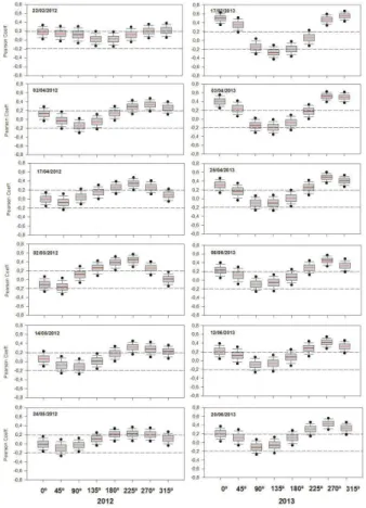
15

Figure 4 shows the correlation between SD and Sx for the eight wind directions at a distance of 200 m (identified as the best correlated searching distance). Despite dif-ferences in magnitude, the correlations for surveys carried out at the beginning of the season in each year showed that SD was clearly affected by N and NW wind directions. This was particularly evident in 2013, as the correlation values were higher. The

con-20

(12)

TCD

8, 1937–1972, 2014

distribution

J. Revuelto et al.

Title Page

Tables Figures

◭ ◮

Back Close

Full Screen / Esc

Discussion

P

a

per

|

D

iscussion

P

a

per

|

Discussion

P

a

per

|

Discuss

ion

P

a

per

during the snow season. In 2013 this phenomenon was less marked because of the greater SD accumulation at the beginning of the snow season accompanied with N di-rection winds, which resulted in only moderate changes in theSx for the most strongly correlated wind directions. It was also observed that in both study years once the snow had started to melt (the last three surveys in each season) the snow distribution did not

5

change in relation toSx directions.

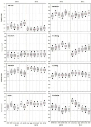
Correlations between the most correlated Sx direction for each day and SD were compared with correlations between SD and the other topographic variables (Fig. 5). This showed thatSx had one of the greatest coefficient of correlation with SD (range 0.18–0.53). The correlations were higher during the accumulation periods, especially

10

in the 2013 snow season, with a reduction in correlations values occurring during the melt period at the end of each snow season.

The TPI at 25 m showed the highest correlation with SD for nearly all of the 12 sampled days. During 2012 the mean correlation values ranged from−0.5 to−0.6 for those surveys during which snow accumulation dominated in the days preceding the

15

surveys. The r _{values were closer to the significance level (}₋_{0.197) for the surveys}

where the preceding days were dominated by melting conditions (14 and 24 May). In 2013, the TPI was more highly correlated with SD than in 2012, with Pearson’s r

coefficients<₋_{0.6 for all survey days.}_Curvature _{also had a high correlation with SD,}

and similar toTPI with a 25 m searching distance was significantly correlated on all the

20

survey dates, but unlike theTPI, the correlation ofCurvaturewith SD did not decrease during the snowmelt periods. The significant correlations ofTPI andCurvaturewith SD highlight the importance of terrain curvature on the SD distribution. The importance of terrain curvature at different scales for SD distribution is clearly evident in Fig. 3, which shows that higher SD values were usually found for concave areas, which showed

25

snow presence until the end of each snow season.

(13)

TCD

8, 1937–1972, 2014

distribution

J. Revuelto et al.

Title Page

Tables Figures

◭ ◮

Back Close

Full Screen / Esc

Discussion

P

a

per

|

D

iscussion

P

a

per

|

Discussion

P

a

per

|

Discuss

ion

P

a

per

|

Slopewas relatively weakly correlated with SD during the 2012 snow season. In 2013 the correlation was greater, and was statistically significant on some days. As with

Elevation, the correlation betweenSlopeand SD was variable between the two study years, and showed a similar temporal pattern toEasting, probably because of the pres-ence of steeper areas on the east-facing slopes.

5

The correlation between Northing and SD was rarely statistically significant, was highly variable, and contributed to explaining SD in a very different ways in 2012 and 2013. In 2012 no correlation between SD andNorthing was found during the accumu-lation period, but during the melting period a slight positive correaccumu-lation was observed, as snow remained longer on north-facing slopes. The 2013 snow season started with

10

a large precipitation event dominated by strong winds from a northerly direction, lead-ing to high levels of snow accumulation on the south-faclead-ing slopes. This explains the strong and statistically significant negative correlation of SD withNorthingfor 17 Febru-ary 2013. This event influenced the rest of the season (as evident in Fig. 4 in 2013), but a progressive decrease in its influence was evident for the following survey days.

Ra-15

diationhad an almost opposite influence on SD to that observed for Northing. During the melting period in each year the Pearson’sr _{correlation between SD and}_Radiation

was negative, indicating a thinner snowpack on the most irradiated slopes; the relation was statistically significant at the end of the 2013 snow season.

4.2 Multiple Linear Regression and Binary Regression Tree models

20

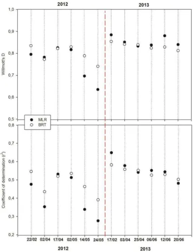
Figure 6 shows the Willmott’sD _{values and the coe}_ffi_{cients of determination (}r2₎

ob-tained in the comparison of observed and predicted values using MLRs and BRTs for an independent dataset (5000 cases) reserved for validation. The MLRs producedr2

values ranging from 0.27 to 0.65 and Willmott’s D _{values ranging from 0.63 to 0.88,}

while the BRTs producedr2_{values ranging from 0.43 to 0.58 and Willmott’s}D_values

25

(14)

TCD

8, 1937–1972, 2014

distribution

J. Revuelto et al.

Title Page

Tables Figures

◭ ◮

Back Close

Full Screen / Esc

Discussion

P

a

per

|

D

iscussion

P

a

per

|

Discussion

P

a

per

|

Discuss

ion

P

a

per

the case for the end of the 2012 season. Overall, the performance of the MLRs was more variable than that of the BRTs, which were more constant amongst the various snow surveys. For those days on which the models were most accurate in predicting SD variability, the MLRs showed slightly better scores than the BRTs. However, for days on which the accuracy between predictions and observations was lower, the BRTs

pro-5

vided better estimates than the MLRs. For 2012, slightly better results were obtained using MLRs, while the opposite occurred in 2013. Nevertheless, only large differences in the accuracy of each model were evident by the end of 2012 snow season, in the two last surveys, which were characterized by thin and patchy snowpack. In general, there was good agreement between the models for each survey day, so results obtained with

10

each model could be compared.

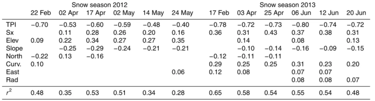
As shown for single correlations, theTPI variable explained most of the variance in MLR models developed for all analyzed days (Table 2). The contribution of the other variables varied markedly among surveys, particularly when the two years were com-pared. In most cases,Elevationwas the second most important variable explaining the

15

SD distribution in 2012, followed bySx and Slope. The other variables made a much smaller contribution, or were not included in the models. The contribution ofElevation

was much less in 2013, and it was not included in three of the six surveys, whereas in 2012 it was included in all surveys. For the entire 2013,Sx was the second most important variable, followed byCurvature, which had an almost negligible influence in

20

2012.Northing was only included in the models for the surveys carried out during pe-riods dominated by snow accumulation, and was not included in the models during the periods dominated by melting.

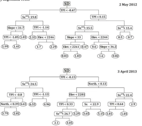
Figure 7 shows two examples of BRTs, obtained for the days 2 May 2012 (upper panel) and 3 April 2013 (bottom panel), which accounted for the largest amount of

25

(15)

TCD

8, 1937–1972, 2014

distribution

J. Revuelto et al.

Title Page

Tables Figures

◭ ◮

Back Close

Full Screen / Esc

Discussion

P

a

per

|

D

iscussion

P

a

per

|

Discussion

P

a

per

|

Discuss

ion

P

a

per

|

and TPI for 2 May 2012, and Sx and Northing for 3 April 2013, demonstrating the importance of these variables in the subsequent branching of the trees.

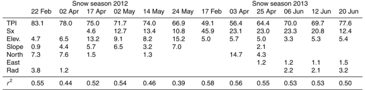
The relative importance (scaled from 0 to 100) of each topographic variable in each BRT is shown in Table 3. This shows that TPI was the first most important variable explaining SD for all survey days. For the 2012 snow season, TPI explained more

5

than 67 % of the total explained variance in all BRTs, and 75 % during the accumu-lation period (the first three surveys). Thus, for most of the survey days the variance explained by the other variables was<_{30 %. The second most important variable}

ex-plaining the SD distribution in 2012 differed amongst the survey days. Thus, Sx was the second most influential variable during May (except for 24 May 2012), following the

10

largest snowfall in the season (which occurred the 1 May 2012), andElevation was the most important variable in the other surveys during 2012.Northing also had an evident influence during the two first surveys of the year, but subsequently had mini-mal explanatory capacity, as was the case for all the other variables. In 2013TPI was also the main contributor to the total explained variance, exceeding 50 % for almost all

15

survey days, and approaching or>_{70 % during the snowmelt period. The influence of}

Sx was more important in 2013 than in the previous year. At the beginning of 2013 the contribution ofSx to the total explained variance was almost 46 %, and remained

>_{20 % for the rest of the snow season; an exception was the last survey, when melting}

dominated and its e_ffect declined to 12 %. When snow was not mobilized for long

pe-20

riods by wind, the SD distribution was more dependent on variables related to terrain curvature (TPI andCurvature). During 2013,Elevationcontributed approximately 5 % to the total explained variance during the entire snow season.Northing made a signif-icant contribution to the model (14.7 %) on only one day (3 April 2013), and a much smaller contribution on the following survey day (25 April 2013). Where included in the

25

(16)

TCD

8, 1937–1972, 2014

distribution

J. Revuelto et al.

Title Page

Tables Figures

◭ ◮

Back Close

Full Screen / Esc

Discussion

P

a

per

|

D

iscussion

P

a

per

|

Discussion

P

a

per

|

Discuss

ion

P

a

per

5 Discussion

The distribution of snow in mountain areas is highly variable in space and time, as was shown for the Izas experimental catchment during two consecutive years. Many me-teorological and topographic parameters a_ffect the snow distribution and its evolution through time. In this context, we demonstrated that topography was a major controlling

5

factor affecting SD in a subalpine catchment, and showed that its effect evolved during the snow accumulation and melting periods over two years having highly contrasting climatic conditions and levels of snow accumulation.

There have been many studies of the spatial distribution of SD in mountain areas (Anderton et al., 2004; Erickson et al., 2005; López-Moreno et al., 2010; Mccreight

10

et al., 2012), but there are very few datasets that have enabled investigation of the intra-and inter-annual occurrence of topographic control on the snowpack distribution. The results of previous research have highlighted the difficulties in fully explaining the dis-tribution of snow in complex mountainous terrain. In addition, the results have differed among studies, and suggest that different variables govern the distribution of

snow-15

pack among areas as consequence of their differing characteristics and geographical settings, including surface area and altitudinal gradients, the importance of wind re-distribution, the presence or absence of vegetation, and the topographic complexity (Grünewald et al., 2013).

Most of the topographic variables investigated in this study have been included

20

in previous studies, including Elevation, Slope, Radiation, Curvature and Sx. Other variables, in particularTPI, have received little attention in previous research (López-Moreno et al., 2010). We showed thatTPI at a scale of 25 m had the greatest capacity to explain the SD distribution in the study catchment.Curvature(which refers to a small spatial scale of terrain curvature) was also highly correlated with the SD distribution,

25

(17)

TCD

8, 1937–1972, 2014

distribution

J. Revuelto et al.

Title Page

Tables Figures

◭ ◮

Back Close

Full Screen / Esc

Discussion

P

a

per

|

D

iscussion

P

a

per

|

Discussion

P

a

per

|

Discuss

ion

P

a

per

|

correlation withCurvatureremained constant. This suggests that snow remains longer in small, deep concavities, but melts faster in wider concave areas that were identified by the 25 mTPI scale. This effect was evident at the end of the snow season, when snow was present only in deep concavities, as shown in Fig. 3. To explain the snow distribution, Anderton et al. (2004) compared the relative elevation of a cell with the

5

terrain over a 40 m radius, and observed that this had a major role on SD distribution, what reinforces curvature importance at different scales.

The maximum upwind slope (Sx; Winstral et al., 2002) has also been identified as a key variable explaining snow distribution, improving the results obtained when it is introduced into models. Our results are consistent with those of other studies that have

10

shown that the optimum searching distance for correlatingSx with the SD distribution is 200 m (Molotch et al., 2005; Schirmer et al., 2011). The Izas experimental catchment does not have a clearly dominant wind direction. For this reason, theSx preferred di-rection for each date was selected, and showed that there were intra-annual shifts in the most highly correlated direction. The change in the most importantSx direction

15

was similar between the 2012 and 2013 snow seasons; it started with a northerly com-ponent and evolved to a dominant westerly direction. We also found a decrease in the correlation between Sx and the snow distribution at the end of each snow sea-son, when melting conditions dominated; this is consistent with the findings of previous studies (Winstral and Marks, 2002).

20

Only for two days (22 February 2012 and 2 April 2012) was there no (or a minor) contribution ofSx to SD, according to the BRTs and MLRs. On these days Northing

was introduced into the models, and was found to explain some of the variance ofSx

from northerly direction (the best correlated direction for these days; Fig. 4).

AlthoughElevation has been found to largely explain the snow distribution in areas

25

(18)

TCD

8, 1937–1972, 2014

distribution

J. Revuelto et al.

Title Page

Tables Figures

◭ ◮

Back Close

Full Screen / Esc

Discussion

P

a

per

|

D

iscussion

P

a

per

|

Discussion

P

a

per

|

Discuss

ion

P

a

per

period the entire catchment is generally above the freezing height. However, during spring the 0◦C isotherm shifts to higher elevations, which may lead to different melt-ing rates within the basin. Despite the relatively weak correlation between Elevation

and SD, this variable was introduced as a predictor in the MLRs and BRTs for most of the days analyzed, as López-Moreno et al. (2010) reported that elevation was of

5

increasing importance as the grid size increased, and Anderton et al. (2004) reported its importance in the same study area. The results of the present study also suggest the importance of Elevation, particularly when considered in combination with other topographic variables.

Slope was only a weak explanatory factor for snow distribution, probably because

10

the slope in most of the catchment is not su_fficient to trigger gravitational movements including avalanches and slushes during the snowmelt period, which could thin the snowpack on the steepest slopes (Elder et al., 1998).

Radiation,NorthingandEastingshowed no close correlation with the snowpack dis-tribution; their relationships with SD were variable over time, with statistically significant

15

correlations occurring on some days and only weak correlations on other days. The re-sults suggested thatRadiationandNorthing (which showed almost opposite patterns) may be related to SD for two different reasons. During the accumulation period in 2013 heavy snowfalls associated with northerly winds led to the accumulation of deep snow on south-facing (more irradiated) surfaces, whereas during the snowmelt period the

20

greater exposure of the southern slopes to solar energy led to a positive (negative) correlation withNorthing (Radiation). This phenomenon was also observed by López-Moreno et al. (2013), using a physically-based snow energy balance model in the same study area. Another effect observed withNorthingwas the contributions of this variable to the MLRs and BRTs only for survey days corresponding to snow accumulation

con-25

(19)

TCD

8, 1937–1972, 2014

distribution

J. Revuelto et al.

Title Page

Tables Figures

◭ ◮

Back Close

Full Screen / Esc

Discussion

P

a

per

|

D

iscussion

P

a

per

|

Discussion

P

a

per

|

Discuss

ion

P

a

per

|

period the negative correlation of this variable with SD was much more evident, pos-sibly due to the increase of the difference in the energetic exchange between the sun exposed and shaded areas. Terrain aspect (mainly Northing) and Radiation during winter were not found to have high explanatory capacity relative to the other variables. Nevertheless, these are useful indicators of the general patterns of snow accumulation

5

processes because of their relation to the dominantSx directions. Thus,Northing and

Radiationare equivalent variables in explaining the SD distribution. More importantly, during winter they were more related to the accumulation patterns resulting from wind redistribution, whereas in spring they were associated with the unequal distribution of solar radiation, which leads to higher melting rates on the most irradiated slopes. Other

10

studies that have comparedNorthing and Radiationhave obtained better simulations when solar radiation was used (Molotch et al., 2005).

The MLRs and BRTs provided reasonably high accuracy scores when observed and predicted SD data were compared. The scores were slightly better than reported in pre-vious research using similar methods, especially as they were obtained from a dataset

15

independent of that used to create the models. One reason for the improvement may be the use of the TPI as a SD predictor, as this variable has not been considered in previous studies. For the 12 survey days theTPIhad the greatest explanatory capacity in both approaches. However, based on comparison of the different dates and sur-veys, the other variables made more varying contributions, as a result of the di_fferent

20

roles they play during the snow accumulation and melting periods, and the wind condi-tions during the main snowfall events. The models had less capacity to explain spatial variability of the snowpack when the snow was thinner and patchy. The BRT and MLR approaches were consistent with respect to error estimates. The results obtained using each approach were comparable, so the trends in the variable ranking for both models

25

(20)

typ-TCD

8, 1937–1972, 2014

distribution

J. Revuelto et al.

Title Page

Tables Figures

◭ ◮

Back Close

Full Screen / Esc

Discussion

P

a

per

|

D

iscussion

P

a

per

|

Discussion

P

a

per

|

Discuss

ion

P

a

per

ical of days when the snowpack is patchy (López-Moreno et al., 2010; Molotch et al., 2005).

The similarity of the models obtained for 2012 and 2013 suggests a consistent inter-annual distribution of the snow pack in the catchment; the areas of maximum SD and the location of snow free zones were consistent between both years of the study. The

5

detected spatial consistency of snowpack has implications for soil dynamics and plant cycles, because some parts of the basin will tend to remain free of snow cover during longer periods favoring the presence of temporary frozen soils, and reducing the iso-lation effect of snowpack to the plants (Keller et al., 2000; Pomeroy and Gray, 1995). Moreover, it suggests that the information acquired from TLS during several years could

10

be useful to design long-term monitoring strategies of SD in the basin based on few manual measurements in representative points according their terrain characteristics.

6 Conclusions

Topographic variables related to terrain curvature were shown to contribute more to ex-plaining snow distribution than other variables. In particular, theTPIat a 25 m searching

15

distance was the major variable explaining SD in the Izas experimental catchment. This suggests the importance of including this index in future snow studies, and the need to establish the best searching distance for relating this variable to SD distribution at other study sites. The maximum upwind slope at a searching distance of 200 m was also an important variable explaining the SD distribution. However, its influence

var-20

ied markedly between years and surveys, depending of the specific wind conditions during the main snowfall events. The influence of the other topographical variables on the spatial distribution of SD was less, and showed greater intra- and inter-annual vari-ability. The results from BRTs and MLRs models were consistent, and the explanatory capacities of the main variables were very similar for all surveys. This suggests that

25

(21)

TCD

8, 1937–1972, 2014

distribution

J. Revuelto et al.

Title Page

Tables Figures

◭ ◮

Back Close

Full Screen / Esc

Discussion

P

a

per

|

D

iscussion

P

a

per

|

Discussion

P

a

per

|

Discuss

ion

P

a

per

|

consistency in the study catchment. Several interesting temporal evolutions during the two snow seasons were found in the relation of some topographic variables to SD.

Acknowledgements. This study was supported by the research project Hidrología nival en el Pirineo Central Español: variabilidad espacial, importancia hidrológica y respuesta a la variabilidad y cambio climático (CGL2011-27536/HID, Hidronieve) “CGL2011-27574-CO2-02

5

and CGL2011-27536, financed by the Spanish Commission of Science and Technology and FEDER; LIFE MEDACC, financed by the LIFE programme of the European Commission”; El glaciar de Monte Perdido: Monitorización y estudio de su dinámica actual y procesos crios-féricos asociados como indicadores de procesos de cambio global844/2013,financed by MA-GRAMA National Parksand CTTP1/12 “Creación de un modelo de alta resolución espacial

10

para cuantificar la esquiabilidad y la afluencia turística en el Pirineo bajo distintos escenarios de cambio climático”, financed by the Comunidad de Trabajo de los Pirineos. The first author is a recipient under the pre-doctoral FPU grant program 2010 (Spanish Ministry of Education Culture and Sports). The third author was the recipient of the postdoctoral grants JAE-DOC043 (CSIC) and JCI-2011-10263 (Spanish Ministry of Science and Innovation). The authors thank

15

Adam Winstral for the use of his algorithm for calculating maximum upwind slope.

References

Anderton, S. P., White, S. M., and Alvera, B.: Evaluation of spatial variability in snow water equivalent for a high mountain catchment, Hydrol. Process., 18, 435–453, 2004.

Bales, R. C. and Harrington, R. F.: Recent progress in snow hydrology, Rev. Geophys., 33,

20

1011–1020, 1995.

Barnett, T. P., Adam, J. C., and Lettenmaier, D. P.: Potential impacts of a warming climate on water availability in snow-dominated regions, Nature, 438, 303–309, 2005.

Beale, C. M., Lennon, J. J., Yearsley, J. M., Brewer, M. J., and Elston, D. A.: Regression analysis of spatial data, Ecol. Lett., 13, 246–264, 2010.

25

Beniston, M.: Climatic change in mountain regions: a review of possible impacts, Climatic Change, 59, 5–31, 2003.

(22)

TCD

8, 1937–1972, 2014

distribution

J. Revuelto et al.

Title Page

Tables Figures

◭ ◮

Back Close

Full Screen / Esc

Discussion

P

a

per

|

D

iscussion

P

a

per

|

Discussion

P

a

per

|

Discuss

ion

P

a

per

Caballero, Y., Voirin-Morel, S., Habets, F., Noilhan, J., LeMoigne, P., Lehenaff, A., and Boone, A.: Hydrological sensitivity of the Adour-Garonne river basin to climate change, Water Resour. Res., 43, W07448, doi:10.1029/2005WR004192, 2007.

Deems, J. S., Fassnacht, S. R., and Elder, K. J.: Fractal distribution of snow depth from Lidar data, J. Hydrometeorol., 7, 285–297, 2006.

5

Deems, J. S., Fassnacht, S. R., and Elder, K. J.: Interannual consistency in fractal snow depth patterns at two Colorado Mountain sites, J. Hydrometeorol., 9, 977–988, 2008.

Del Barrio, G., Alvera, B., Puigdefabregas, J., and Diez, C.: Response of high mountain land-scape to topographic variables: Central Pyrenees, Landland-scape Ecol., 12, 95–115, 1997. Egli, L., Jonas, T., Grünewald, T., Schirmer, M., and Burlando, P.: Dynamics of snow ablation in

10

a small Alpine catchment observed by repeated terrestrial laser scans, Hydrol. Process., 26, 1574–1585, 2012.

Elder, K., Dozier, J., and Michaelsen, J.: Snow accumulation and distribution in an Alpine Wa-tershed, Water Resour. Res., 27, 1541–1552, 1991.

Elder, K., Rosenthal, W., and Davis, R. E.: Estimating the spatial distribution of snow water

15

equivalence in a montane watershed, Hydrol. Process., 12, 1793–1808, 1998.

Erickson, T. A., Williams, M. W., and Winstral, A.: Persistence of topographic controls on the spatial distribution of snow in rugged mountain terrain, Colorado, United States, Water Re-sour. Res., 41, 1–17, 2005.

Erxleben, J., Elder, K., and Davis, R.: Comparison of spatial interpolation methods for

estimat-20

ing snow distribution in the Colorado Rocky Mountains, Hydrol. Process., 16, 3627–3649, 2002.

Fassnacht, S. R. and Deems, J. S.: Measurement sampling and scaling for deep montane snow depth data, Hydrol. Process., 20, 829–838, 2006.

Fassnacht, S. R., Dressler, K. A., and Bales, R. C.: Snow water equivalent interpolation for

25

the Colorado River Basin from snow telemetry (SNOTEL) data, Water Resour. Res., 39, SWC31–SWC310, 2003.

Fassnacht, S. R., López-Moreno, J. I., Toro, M., and Hultstrand, D. M.: Mapping snow cover and snow depth across the Lake Limnopolar watershed on Byers Peninsula, Livingston Island, Maritime Antarctica, Antarct. Sci., 25, 157–166, 2013.

30

(23)

TCD

8, 1937–1972, 2014

distribution

J. Revuelto et al.

Title Page

Tables Figures

◭ ◮

Back Close

Full Screen / Esc

Discussion

P

a

per

|

D

iscussion

P

a

per

|

Discussion

P

a

per

|

Discuss

ion

P

a

per

|

Groffman, P. M., Driscoll, C. T., Fahey, T. J., Hardy, J. P., Fitzhugh, R. D., and Tierney, G. L.: Colder soils in a warmer world: a snow manipulation study in a northern hardwood forest ecosystem, Biogeochemistry, 56, 135–150, 2001.

Grünewald, T., Schirmer, M., Mott, R., and Lehning, M.: Spatial and temporal variability of snow depth and ablation rates in a small mountain catchment, The Cryosphere, 4, 215–225,

5

doi:10.5194/tc-4-215-2010, 2010.

Grünewald, T., Stötter, J., Pomeroy, J. W., Dadic, R., Moreno Baños, I., Marturià, J., Spross, M., Hopkinson, C., Burlando, P., and Lehning, M.: Statistical modelling of the snow depth distri-bution in open alpine terrain, Hydrol. Earth Syst. Sci., 17, 3005–3021, doi:10.5194/hess-17-3005-2013, 2013.

10

Hair, J. F., Anderson, R., Tatham, R., and Black, W.: Multivariate Data Analysis, Printice Hall, Upper Saddle River, New Jersey, USA, 1998.

Hosang, J. and Dettwiler, K.: Evaluation of a water equivalent of snow cover map in a small catchment area using a geostatistical approach, Hydrol. Process., 5, 283–290, 1991. Jost, G., Weiler, M., Gluns, D. R., and Alila, Y.: The influence of forest and topography on snow

15

accumulation and melt at the watershed-scale, J. Hydrol., 347, 101–115, 2007.

Keller, F., Kienast, F., and Beniston, M.: Evidence of response of vegetation to environmental change on high-elevation sites in the Swiss Alps, Reg. Environ. Change, 1, 70–77, 2002. Lehning, M., Löwe, H., Ryser, M., and Raderschall, N.: Inhomogeneous precipitation

distribution and snow transport in steep terrain, Water Resour. Res., 44, W07404,

20

doi:10.1029/2007WR006545, 2008.

Liston, G. E.: Interrelationships among snow distribution, snowmelt, and snow cover deple-tion: implications for atmospheric, hydrologic, and ecologic modeling, J. Appl. Meteorol., 38, 1474–1487, 1999.

López-Moreno, J. I. and Nogués-Bravo, D.: A generalized additive model for the spatial

distri-25

bution of snowpack in the Spanish Pyrenees, Hydrol. Process., 19, 3167–3176, 2005. López-Moreno, J. I., Latron, J., and Lehmann, A.: Effects of sample and grid size on the

ac-curacy and stability of regression-based snow interpolation methods, Hydrol. Process., 24, 1914–1928, 2010.

López-Moreno, J. I., Vicente-Serrano, S. M., Morán-Tejeda, E., Lorenzo-Lacruz, J., Kenawy, A.,

30

(24)

TCD

8, 1937–1972, 2014

distribution

J. Revuelto et al.

Title Page

Tables Figures

◭ ◮

Back Close

Full Screen / Esc

Discussion

P

a

per

|

D

iscussion

P

a

per

|

Discussion

P

a

per

|

Discuss

ion

P

a

per

López-Moreno, J. I., Fassnacht, S. R., Heath, J. T., Musselman, K. N., Revuelto, J., Latron, J., Morán-Tejeda, E., and Jonas, T.: Small scale spatial variability of snow density and depth over complex alpine terrain: implications for estimating snow water equivalent, Adv. Water Resour., 55, 40–52, 2012a.

López-Moreno, J. I., Pomeroy, J. W., Revuelto, J., and Vicente-Serrano, S. M.: Response of

5

snow processes to climate change: spatial variability in a small basin in the Spanish Pyre-nees, Hydrol. Process., 27, 2637–2650, 2012b.

McCreight, J. L., Slater, A. G., Marshall, H. P., and Rajagopalan, B.: Inference and uncertainty of snow depth spatial distribution at the kilometre scale in the Colorado Rocky Mountains: the effects of sample size, random sampling, predictor quality, and validation procedures,

10

Hydrol. Process., 28, 933–957, 2014.

Molotch, N. P. and Bales, R. C.: Scaling snow observations from the point to the grid el-ement: implications for observation network design, Water Resour. Res., 41, W11421, doi:10.1029/2005WR004229, 2005.

Molotch, N. P., Colee, M. T., Bales, R. C., and Dozier, J.: Estimating the spatial distribution of

15

snow water equivalent in an alpine basin using binary regression tree models: the impact of digital elevation data and independent variable selection, Hydrol. Process., 19, 1459–1479, 2005.

Mott, R., Schirmer, M., Bavay, M., Grünewald, T., and Lehning, M.: Understanding snow-transport processes shaping the mountain snow-cover, The Cryosphere, 4, 545–559,

20

doi:10.5194/tc-4-545-2010, 2010.

Mott, R., Schirmer, M., and Lehning, M.: Scaling properties of wind and snow depth distribution in an Alpine catchment, J. Geophy. Res.-Atmos., 116, D06106, doi:10.1029/2010JD014886, 2011.

Pomeroy, J. W. and Gray, D. M.: Snowcover Accumulation, Relocation, and Management,

Na-25

tional Hydrological Research Institute, Saskatoon, Sask., Canada, 1995.

Pomeroy, J., Essery, R., and Toth, B.: Implications of spatial distributions of snow mass and melt rate for snow-cover depletion: observations in a subarctic mountain catchment, Ann. Glaciol., 38, 195–201, 2004.

Prokop, A.: Assessing the applicability of terrestrial laser scanning for spatial snow depth

mea-30

(25)

TCD

8, 1937–1972, 2014

distribution

J. Revuelto et al.

Title Page

Tables Figures

◭ ◮

Back Close

Full Screen / Esc

Discussion

P

a

per

|

D

iscussion

P

a

per

|

Discussion

P

a

per

|

Discuss

ion

P

a

per

|

Prokop, A., Schirmer, M., Rub, M., Lehning, M., and Stocker, M.: A comparison of measurement methods: terrestrial laser scanning, tachymetry and snow probing for the determination of the spatial snow-depth distribution on slopes, Ann. Glaciol., 49, 210–216, 2008.

Revuelto, J., López-Moreno, J. I., Azorin-Molina, C., Zabalza, J., Arguedas, G., and Vicente-Serrano, S. M.: Mapping the annual evolution of snow depth in a small catchment in

5

the Pyrenees using the long-range terrestrial laser scanning, J. Maps, 10, 379–393, doi:10.1080/17445647.2013.869268, 2014.

Schaffhauser, A., Adams, M., Fromm, R., Jörg, P., Luzi, G., Noferini, L., and Sailer, R.: Remote sensing based retrieval of snow cover properties, Cold Reg. Sci. Technol., 54, 164–175, 2008.

10

Schirmer, M. and Lehning, M.: Persistence in intra-annual snow depth distribution: 2. Fractal analysis of snow depth development, Water Resour. Res., 47, W09517, doi:10.1029/2010WR009429, 2011.

Schirmer, M., Wirz, V., Clifton, A., and Lehning, M.: Persistence in intra-annual snow depth distribution: 1. Measurements and topographic control, Water Resour. Res., 47, W09516,

15

doi:10.1029/2010WR009426„ 2011.

Scipión, D. E., Mott, R., Lehning, M., Schneebeli, M., and Berne, A.: Seasonal small-scale spatial variability in alpine snowfall and snow accumulation, Water Resour. Res., 49, 1446– 1457, 2013.

Steger, C., Kotlarski, S., Jonas, T., and Schär, C.: Alpine snow cover in a changing climate:

20

a regional climate model perspective, Clim. Dynam., 41, 735–754, 2012.

Trujillo, E., Ramírez, J. A., and Elder, K. J.: Topographic, meteorologic, and canopy controls on the scaling characteristics of the spatial distribution of snow depth fields, Water Resour. Res., 43, W07409, doi:10.1029/2006WR005317, 2007.

Watson, F. G. R., Anderson, T. N., Newman, W. B., Alexander, S. E., and Garrott, R. A.: Optimal

25

sampling schemes for estimating mean snow water equivalents in stratified heterogeneous landscapes, J. Hydrol., 328, 432–452, 2006.

Weiss, A. D.: Topographic Position and Landforms Analysis, ESRI User Conference, San Diego, USA, 2001.

Willmott, C. J.: On the validation of models, Phys. Geogr., 2, 184–194, 1981.

30

(26)

TCD

8, 1937–1972, 2014

distribution

J. Revuelto et al.

Title Page

Tables Figures

◭ ◮

Back Close

Full Screen / Esc

Discussion

P

a

per

|

D

iscussion

P

a

per

|

Discussion

P

a

per

|

Discuss

ion

P

a

per

Winstral, A., Elder, K., and Davis, R. E.: Spatial snow modeling of wind-redistributed snow using terrain-based parameters, J. Hydrometeorol., 3, 524–538, 2002.

Wipf, S., Stoeckli, V., and Bebi, P.: Winter climate change in alpine tundra: plant responses to changes in snow depth and snowmelt timing, Climatic Change, 94, 105–121, 2009.

Zar, J. H.: Biostatistical Analysis, 2nd. edn., Prentice Hall, Englewood Cliffs, New Jersey, USA,

5

(27)

TCD

8, 1937–1972, 2014

distribution

J. Revuelto et al.

Title Page

Tables Figures

◭ ◮

Back Close

Full Screen / Esc

Discussion

P

a

per

|

D

iscussion

P

a

per

|

Discussion

P

a

per

|

Discuss

ion

P

a

per

|

Table 1.Summary statistics of the snowpack distribution and the snow covered area of the

basin. Note that snow covered area is expressed as a % of the total area surveyed by the TLS, and the mean SD is the average of all SDs not including zero values.

Snow season 2012 Snow season 2013

(28)

TCD

8, 1937–1972, 2014

distribution

J. Revuelto et al.

Title Page

Tables Figures

◭ ◮

Back Close

Full Screen / Esc

Discussion

P

a

per

|

D

iscussion

P

a

per

|

Discussion

P

a

per

|

Discuss

ion

P

a

per

Table 2.Multiple linear regression beta coefficients for each independent variable and sampled

day.

22 Feb 02 Apr 17 Apr 02 May 14 May 24 May 17 Feb 03 Apr 25 Apr 06 Jun 12 Jun 20 Jun

TPI −0.70 −0.53 −0.60 −0.59 −0.48 −0.40 −0.78 −0.72 −0.73 −0.80 −0.74 −0.72

Sx 0.11 0.28 0.26 0.20 0.16 0.36 0.31 0.43 0.37 0.38 0.31

Elev 0.09 0.22 0.34 0.27 0.27 0.35 0.14 0.08 0.13

Slope −0.25 −0.29 −0.24 −0.21 −0.21 −0.10 −0.14 −0.16 −0.09 −0.15

North −0.22 0.13 −0.16 −0.12 −0.11 −0.11

Curv. 0.10 0.29 0.25 0.25 0.31 0.23 0.20

East 0.06 0.12 0.08 0.07 0.07

Rad 0.08 0.08 0.07

(29)

TCD

8, 1937–1972, 2014

distribution

J. Revuelto et al.

Title Page

Tables Figures

◭ ◮

Back Close

Full Screen / Esc

Discussion

P

a

per

|

D

iscussion

P

a

per

|

Discussion

P

a

per

|

Discuss

ion

P

a

per

|

Table 3. Contribution of the various topographic variables to the explained variance of SD

distribution in the binary regression models for 2012 and 2013. Values have been rescaled from 0 to 100.

22 Feb 02 Apr 17 Apr 02 May 14 May 24 May 17 Feb 03 Apr 25 Apr 06 Jun 12 Jun 20 Jun

TPI 83.1 78.0 75.0 71.7 74.0 66.9 49.1 56.4 64.4 70.0 69.7 77.6

Sx 4.6 12.7 13.4 10.8 45.9 23.1 23.0 23.3 20.8 12.4

Elev. 4.7 6.5 13.2 9.1 8.2 15.2 5.0 5.7 5.0 3.3 5.3 5.4

Slope 0.9 4.4 5.7 6.5 3.2 7.0 2.1

North 7.3 7.6 1.5 1.3 14.7 4.3

East 1.2 1.2 1.1 1.5

Rad 3.8 1.2 2.2 2.1 3.2

(30)

TCD

8, 1937–1972, 2014

distribution

J. Revuelto et al.

Title Page

Tables Figures

◭ ◮

Back Close

Full Screen / Esc

Discussion

P

a

per

|

D

iscussion

P

a

per

|

Discussion

P

a

per

|

Discuss

ion

P

a

per

Fig. 1.Location of the Izas experimental catchment, and the digital elevation model showing