Impacts of climate and emission changes on nitrogen deposition in Europe: a multi-model study

www.atmos-chem-phys.net/14/6995/2014/ doi:10.5194/acp-14-6995-2014

© Author(s) 2014. CC Attribution 3.0 License.

Impacts of climate and emission changes on nitrogen deposition in

Europe: a multi-model study

D. Simpson1,2, C. Andersson3, J.H. Christensen4, M. Engardt3, C. Geels4, A. Nyiri1, M. Posch5, J. Soares6, M. Sofiev6, P. Wind1,7, and J. Langner3

1_{EMEP MSC-W, Norwegian Meteorological Institute, Oslo, Norway}

2_{Dept. Earth & Space Sciences, Chalmers University of Technology, Gothenburg, Sweden} 3_{Swedish Meteorological and Hydrological Institute, Norrköping, Sweden}

4_{Department of Environmental Science, Aarhus University, 4000 Roskilde, Denmark}

5_{National Institute for Public Health and the Environment (RIVM), Bilthoven, the Netherlands} 6_{Finnish Meteorological Institute, P.O. Box 503, 00101 Helsinki, Finland}

7_{University of Tromsø, 9037 Tromsø, Norway}

Correspondence to:D. Simpson (david.simpson@met.no)

Received: 28 January 2014 – Published in Atmos. Chem. Phys. Discuss.: 13 March 2014 Revised: 16 May 2014 – Accepted: 2 June 2014 – Published: 9 July 2014

Abstract. The impact of climate and emissions changes on the deposition of reactive nitrogen (Nr) over Europe was studied using four offline regional chemistry transport mod-els (CTMs) driven by the same global projection of future cli-mate over the period 2000–2050. Anthropogenic emissions for the years 2005 and 2050 were used for simulations of both present and future periods in order to isolate the im-pact of climate change, hemispheric boundary conditions and emissions, and to assess the robustness of the results across the different models.

The results from these four CTMs clearly show that the main driver of future N-deposition changes is the specified emission change. Under the specified emission scenario for 2050, emissions of oxidised nitrogen were reduced substan-tially, whereas emissions of NH3 increase to some extent,

and these changes are largely reflected in the modelled con-centrations and depositions. The lack of sulfur and oxidised nitrogen in the future atmosphere results in a much larger fraction of NHxbeing present in the form of gaseous

ammo-nia.

Predictions for wet and total deposition were broadly con-sistent, although the three fine-scale models resolve Euro-pean emission areas and changes better than the hemispheric-scale model. The biggest difference in the models is for pre-dictions of individual N compounds. One model (EMEP) was used to explore changes in critical loads, also in

conjunc-tion with speculative climate-induced increases in NH3

emis-sions. These calculations suggest that the area of ecosystems that exceeds critical loads is reduced from 64 % for year 2005 emissions levels to 50 % for currently estimated 2050 levels. A possible climate-induced increase in NH3emissions could

worsen the situation, with areas exceeded increasing again to 57 % (for a 30 % NH3emission increase).

1 Introduction

As noted in Langner et al. (2012b), air pollution is still a ma-jor problem in Europe, with levels of gases and particles fre-quently exceeding target values. Many sensitive ecosystems are adversely affected by deposition of reactive nitrogen (Nr) from the atmosphere to vegetation and water bodies (Eris-man et al., 2013; Sutton et al., 2011). Nr comprises both oxi-dised and reduced compounds, generally indicated by NOy

and NHx respectively. Important NOy compounds include

NO and NO2 (together known as NOx) as well as species

such as HNO3 or particulate nitrates. The dominant NHx

compounds are gaseous ammonia (NH3) and particulate

am-monium, the latter usually associated with either sulfates or nitrate. Although emissions of NOxin Europe are expected

to keep decreasing in the future, emissions of NH3may well

realisation is that increased temperatures associated with cli-mate change may induce additional NH3emissions through

increased evaporation (Skjøth and Geels, 2013; Sutton et al., 2013); these studies suggest possible increases of 20–50 % over the next century.

Changes in atmospheric circulation due to climate change can also affect future levels of air pollution and Nr deposi-tion (e.g. Engardt and Langner, 2013, and references cited therein). Changes in meteorological conditions further influ-ence local dispersion and deposition conditions to vegetation and thereby influence the effects of both long-range trans-ported and locally emitted air pollutants on human health and ecosystems. Since the 1990s the concentration of S compo-nents in the Arctic has declined, while the pattern for N com-ponents is more complex, showing both positive and negative trends. These interannual variations reflect the significant re-ductions in sulfur emissions in North America and Europe as well as interannual variations in synoptic transport and pre-cipitation (Hole et al., 2009).

The link between climate change and air pollution in Eu-rope has been assessed in several recent studies using re-gional chemistry transport models (CTMs) (e.g. Langner et al., 2005, 2012a, b; Forkel and Knoche, 2007; Hedegaard et al., 2008; Andersson and Engardt, 2010; Colette et al., 2012; Engardt and Langner, 2013). The majority of these studies have focused on ozone concentrations, but, for exam-ple, Hole and Engardt (2008), Langner et al. (2009), Hede-gaard et al. (2013) and Engardt and Langner (2013) pre-sented some results for nitrogen species. Likewise, a number of studies have made projections of the future N deposition in Europe and the Arctic which included emission changes (e.g. Hole et al., 2009; Geels et al., 2012b; Engardt and Langner, 2013; Tuovinen et al., 2013, the latter using EMEP model results from the present exercise).

Several multi-model studies of atmospheric chemistry and long-range transport of air pollution in Europe have been car-ried out over the last decade (e.g. Vautard et al., 2006, 2007; van Loon et al., 2007; Cuvelier et al., 2007; Thunis et al., 2007; Colette et al., 2011; Solazzo et al., 2012; Dore et al., 2013), also at the hemispheric scale (Dentener et al., 2006; Sanderson et al., 2008). These studies have focused on es-tablishing the robustness of model predictions in the present climate, although Lamarque et al. (2005) used global-scale models with projections up to 2100.

Here we assess the combined uncertainty of predicting fu-ture climate, emissions and atmospheric chemistry as well as long-range transport of Nr over Europe, using finer-scale cli-mate projections than used in previous studies, and with mon emissions and meteorological systems. This study com-plements that of Engardt and Langner (2013), which used one CTM (MATCH) and examined the effects of using dif-ferent meteorological drivers. Here we take a multi-model approach using four state-of-the-art offline CTMs to assess the uncertainty/robustness of model predictions of nitrogen deposition over Europe. Specifically, we evaluate the

sensi-tivity of simulated Nr deposition over Europe to changes in climate, changes in boundary conditions, and to emissions.

This study is a follow-up to the ozone study of Langner et al. (2012b), and largely follows the same methodology ex-cept in three respects: (i) the emission inventories were up-dated (see Sect. 2.1), making use of recent improvements in data sets and finer-scale spatial distributions to provide more accurate model inputs; (ii) we have investigated the effects of emissions changes as well as of climate change; and (iii) 20 yr time windows of simulation were considered instead of 10 yr. The choice of 20 yr time windows was primarily driven by the strong interannual variability in precipitation and re-sulting interannual variability in wet deposition in the CTMs. Using shorter simulation periods leads to deposition changes driven by climate change that are not significant for large ar-eas of the simulation domain. The use of 20 yr time windows also smoothes some of the decadal variability present in the climate model output. An even longer time window could have been considered, but 20 yr was found to be a good com-promise between computational effort and level of signifi-cance.

2 Methods

This study uses the same basic model chain as in the ozone study of Langner et al. (2012b). Briefly, we focus on the comparison of Nr simulations from three European-scale CTMs (EMEP MSC-W, MATCH and SILAM) and one hemispheric CTM (DEHM). In order to obtain climate-sensitive meteorology, meteorological data from a global cli-mate model (GCM) were used in both a regional clicli-mate model (RCM) and an offline hemispheric chemical trans-port model (DEHM). The downscaled meteorology from the RCM is used together with time-varying boundary condi-tions from the hemispheric DEHM CTM to drive the three European-scale CTMs. The horizontal grid for these CTMs was identical to the RCA3 grid, while the vertical discretisa-tion was left free to each model.

Table 1.Model runs used in this study.

Label Emis. Meteor. BIC label DEHM setup Comment

E05-M00-BC1 2005 1990–2009 BC1 E05-M00 Base case – current conditions E05-M50-BC2 2005 2040–2059 BC2 E05-M50 Climate change only

E05-M50-BC3 2005 2040–2059 BC3 E50-M50 Climate+boundary condition changes E50-M50-BC3 2050 2040–2059 BC3 E50-M50 Future conditions

E50X20-M50-BC3 2050 2040–2059 BC3 E50-M50 20 % more NH₃, EMEP, DEHM only E50X30-M50-BC3 2050 2040–2059 BC3 E50-M50 30 % more NH₃, EMEP only

Notes: the BIC label is shorthand for the boundary and initial conditions provided by the DEHM model using the setup for emissions and meteorology given here; see Sect. 2.

Two final scenarios are included in Table 1, E50X20-M50-BC3 and E50X30-M50-E50X20-M50-BC3, both of which are run with just one or two models as a more speculative exercise. These sce-narios are added in order to address the possible increased emissions of ammonia resulting from increased temperatures (Skjøth and Geels, 2013; Sutton et al., 2013). This exercise will be discussed in Sects. 2.1.1 and 4. Details of the emis-sion data, scenarios and models follow.

2.1 Emissions

The models used in this study require emissions of sulfur and nitrogen oxides (SOx, NOx), NH3, non-methane volatile

or-ganic compounds (NMVOCs), and CO, and CH4for DEHM.

The anthropogenic emissions consist of annual, gridded data sets. Ten major types of anthropogenic emissions are used, classified with the so-called “SNAP”-level emission sectors (SNAP stands for Source Nomenclature of Air Pollutants; for example, SNAP-7 is road traffic, SNAP-10 is agriculture, etc.).

In this study, all models made use of the same emission files, which contained gridded SNAP-level data on the RCA3 grid (and a global grid for DEHM). A number of emission inventories that became available in 2012 were merged for this study, aiming to provide consistency with databases used within the EU ECLAIRE project (http://www.eclaire-fp7. eu/) and best-possible spatial resolution for the underlying data. The latter aspect is important as the emissions need to be interpolated to the rotated latitude–longitude grid system of the RCA model, and the finer the base grid, the more ac-curate such interpolation can be.

A three-step procedure was used to generate the com-mon emissions database used by all models. Firstly, the main database, supplying national SNAP-sector emissions for all countries, consists of the so-called ECLIPSE data as pro-duced by the International Institute for Applied System Anal-ysis (IIASA). These data, for both 2005 and 2050, were pro-duced for the EU ECLIPSE project (e.g. Stohl et al., 2013) and the Task Force on Hemispheric Transport of Air Pol-lution (Amann et al., 2013). The original (ECLIPSE v.4) databases produced in 2012 were updated in February 2013

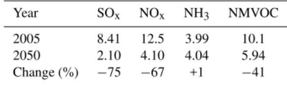
Table 2.Emissions for EU28+used in the calculations for 2005 and

2050. Data from the IIASA/ECLIPSE v.4e_{data set; see text. Unit:}

Tg yr−1_{(SOxas SO2, NOxas NO2).}

Year SOx NOx NH3 NMVOC

2005 8.41 12.5 3.99 10.1 2050 2.10 4.10 4.04 5.94 Change (%) −75 −67 +1 −41

Notes: EU28+_{here denotes the 28 EU countries, plus Norway and} Switzerland.

for the ECLAIRE project; we denote these data as ECLIPSE v.4e_{. Secondly, for countries within the so-called MACC area} (this includes all of the EU, plus some neighbours), the 7 km resolution MACC-2 emissions produced by TNO (Kuenen et al., 2011) were used to spatially distribute the country-specific SNAP emissions. For other countries the IIASA 0.5◦_×0.5◦ _{spatial resolution was preserved. Finally,} inter-national shipping emissions were added from the RCP6.0 data sets (Hijioka et al., 2008). This scenario was cho-sen in discussion with IIASA as most appropriate for the ECLIPSE/ECLAIRE assumptions.

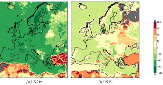
Emission data sets using this procedure were provided for the years 2005 and a 2050 “current legislation” (CLE) sce-nario. The EU totals are presented in Table 2. Figure 1 il-lustrates the 2005 emissions for NOxand NH3in the RCA3

domain used by the three European-scale CTMs, and Fig. 2 shows the changes in emissions between 2005 and 2050. The changes for NOxare dramatic across almost the whole EU

area. In Germany, for example, emissions decrease by nearly 70 %. Dramatic emissions increases are also seen in some ar-eas, especially in northern Africa and Turkey. For NH3, the

emission changes are more complex, with increases and de-creases even within the EU area, and dramatic inde-creases in some Russian areas especially.

Figure 1.Emissions of NOxand NH3for the 2005 base year. Unit: kg(N)ha−1. Also indicated is the transect line through 10◦E used in

Figs. 4, 8 and 9.

Figure 2.Emissions changes (%), 2005 to 2050, of NOxand NH3.

projections assume business-as-usual economic development and implementation of all currently agreed emission control legislation (cf. Amann et al., 2012, 2013). They also make much more use of detailed national data, and are believed more appropriate than RCP for air quality modelling. How-ever, the large (67 %) NHxemission reductions seen in

Ta-ble 2 are broadly consistent with RCP changes for EU27 presented in Winiwarter et al. (2011). Emissions of NHxare

predicted to remain almost constant in Table 2, whereas RCP estimates suggest either a significant increase (ca. 25% for RCP8.5) or decrease (ca. 25 % for RCP2.6 and RCP4.5). There are of course considerable uncertainties in all these projections, arising from assumptions concerning technical measures, growth and policies (Amann et al., 2013).

A number of other emissions sources are typically used in the CTMs. These include so-called natural NOx emissions

from soils; NMVOC from vegetation; and emissions from

forest fires, aircraft and lightning. The CTMs have differ-ent approaches to these emissions sources, and harmonising these was beyond the scope of our study. Instead, in order to simplify the interpretation of the CTM results, we have adopted the simple policy of setting emissions from soils, forest fires, aircraft and lightning to zero, so that all NOx

emissions in the models stem from the common emission data set discussed above. In contrast to these minor emission sources, emissions of NMVOC from vegetation are too great to ignore (e.g. Simpson et al., 1999), and as in Langner et al. (2012b), each model simply calculates its own emissions at each model time step (differences in isoprene emissions were indeed substantial, ranging from ca. 1600 to 8000 Gg yr−1_as

The official EMEP estimate of volcanic emissions was used for all models.

2.1.1 A possible future – increased NH3emissions? Two recent papers have drawn attention to the possibility of quite significant increases in NH3emissions in the future as

a result of increasing evaporation from sources such as an-imal manure. These emissions are a function of both water availability and temperature with, in principle, a doubling of the emission for each 5◦_{C increase. Sutton et al. (2013),} using empirical models and measurements, estimated a po-tential 42 % increase in the global NH3 emissions

follow-ing a 5◦_{C increase towards 2100. Skjøth and Geels (2013)} used a dynamic NH3emission model (Skjøth et al., 2011) to

study the temporal and geographical variations in ammonia emissions across the northern part of Europe. By using bias-corrected ensemble mean surface temperatures from the EN-SEMBLES project (van der Linden and Mitchell, 2009), the potential future changes in the emission from a typical Dan-ish pig stable were tested in different locations and hence climates. Towards the 2050s a general increase of 15–30 % (relative to 2007) was found in the emissions in central to northern Europe, increasing to ca. 20–40 % by the end of the century. It is reasonable to postulate that such increased emis-sions have the potential to partially offset many of the benefi-cial effects of European NOyemissions reductions. The fact

that more NHxwill be in the form of NH3rather than NH+₄

(see Sect. 3.4) also suggests the possibility of quite large in-creases in near-source deposition if such emissions inin-creases occur. The projected increase will of course depend heavily on the projected temperature change and hence on the ap-plied climate model, as well as assumptions concerning NH3

emission factors. However, based on the above studies we have chosen to explore the potential impact of a 20 and 30 % increase in NH3 emissions in our future period 2040–2059

in two scenarios denoted E50X20-M50-BC3 and E50X30-M50-BC3 (Table 1). Given the speculative nature of this ex-ercise, we have used just the DEHM (for 20 %) and EMEP (for 20 and 30 %) models, with a focus on the impact of these scenarios on the critical loads calculations we will present in Sect. 4.

2.2 Climate meteorology

Results of the global-scale ECHAM5 general circulation model (GCM) (Roeckner et al., 2006), driven by emissions from the SRES A1B scenario (Naki´cenovi´c, 2000), were downscaled over Europe with the Rossby Centre Regional Climate model (RCM) version 3 (RCA3) (Samuelsson et al., 2011; Kjellstrom et al., 2011). Details and discussion of both current and future climate simulated with RCA3 are given in Samuelsson et al. (2011) and Kjellstrom et al. (2011). Here we used the so-called ECHAM5-r3 downscaling from the SRES A1B emission scenario (see Kjellstrom et al., 2011, for

details). The ECHAM5 version used is defined in a spectral grid with truncation T63, which at mid-latitudes corresponds to a horizontal resolution of ca. 140 km×210 km. The tem-poral resolution of the climate data was 6 hourly.

As in Langner et al. (2012b), the horizontal resolution of RCA3 was 0.44◦×0.44◦ (ca. 50 km×50 km) on a ro-tated latitude–longitude grid, and data were provided with 6-hourly resolution. The climate as downscaled by RCA3 re-flects broad features of the climate simulated by the parent GCM. The average temperature change in the period 2000– 2040 predicted by RCA3 for the European model domain in the downscaled ECHAM5-r3 is 1.27◦_{C. Until the period} 2040–2070, this climate projection has a temperature change close to the average of an ensemble of 16 different projec-tions downscaled from different GCM runs by RCA3 over Europe (Kjellstrom et al., 2011).

Figures S1 and S2 (see Supplement) illustrate the changes in temperature and precipitation between our 20 yr time slices, from both the ECHAM-5 and RCA3 data. Although the general patterns of temperature are similar, the RCA3 temperature has clearly a higher spatial resolution than the ECHAM5 data, which is particularly obvious over the Alpine area. Temperature increases up to the 2050s are somewhat greater in the ECHAM5 system.

For precipitation the increased resolution of RCA3 is also very evident. ECHAM5 has substantially more rainfall over most of Europe, but less so in some areas, e.g. western Nor-way or the Alps. However both models show rather similar large-scale changes in precipitation to the 2050s, with rather large increases (ca. 10 %) in north-eastern Europe, and de-creases of around 10 % around the Mediterranean.

2.3 Chemical boundary conditions

As in Langner et al. (2012b), chemical boundary conditions at lateral and top boundaries of the regional models were provided by the hemispheric DEHM model, which was also driven by the global ECHAM5-r3 meteorology. The bound-ary values taken from DEHM were updated every 6 h and interpolated from the DEHM resolution to the respective ge-ometry of each regional CTM. To ensure consistency, the offline DEHM model was operated with global emissions for 2005 and 2050 from the same system as used for the European-scale CTMs.

2.4 The chemical transport models

2.4.1 DEHM

The Danish Eulerian Hemispheric Model (DEHM) is a three-dimensional, Eulerian CTM (Christensen, 1997; Frohn et al., 2002; Brandt et al., 2012; Geels et al., 2012a) developed at the Danish National Environmental Research Institute (now Aarhus University). The model domain covers most of the Northern Hemisphere, discretised on a polar stereographic projection, and includes a two-way nesting procedure with several nests with higher resolution over Europe, northern Europe and Denmark (Frohn et al., 2002). In the verti-cal the model has 20 unevenly distributed layers defined in a terrain-following sigma-level coordinate system with a top at 100 hPa.

The chemical scheme comprises 58 photo-chemical com-pounds, 9 classes of particulate matter and 122 chemical re-actions. The original scheme by Strand and Hov (1994) has been extended to include species relevant for the ammonium group chemistry. This includes ammonia (NH3),

ammo-nium nitrate (NH4NO3), ammonium bisulfate (NH4HSO4),

ammonium sulfate ((NH4)2SO4) and inorganic nitrates.

Gaseous and aerosol dry-deposition velocities are calculated based on the resistance method and are parameterised sim-ilar to the EMEP model (Simpson et al., 2003a; Emberson et al., 2000a) except for the dry deposition of species on wa-ter surfaces where the deposition depends on the solubility of the chemical species and the wind speed (Asman et al., 1994; Hertel et al., 1995). Wet deposition includes in-cloud and below-cloud scavenging and is calculated as the product of scavenging coefficients and the concentration in air.

Natural emissions of isoprene are calculated dynamically in the model according to the IGAC-GEIA biogenic emis-sion model (International Global Atmospheric Chemistry – Global Emission Inventory Activity) (Guenther et al., 1995). Background CH4 concentrations were assumed to be

1760 ppb in all scenarios. As well as simplifying the interpre-tation of changes, this is consistent with John et al. (2012), who suggest that the atmospheric CH4 is not projected to

change much under all but the most extreme RCP scenarios. DEHM is regularly validated against observations of, for ex-ample, acidifying and eutrophying compounds (Brandt et al., 2012; Geels et al., 2012b, 2005).

2.4.2 EMEP MSC-W

The gaseous nitrogen species in the EMEP model that are subject to dry deposition are NO2, HNO2, HNO3, PAN,

MPAN and NH3 (see Simpson et al., 2012, for explanation

of PAN species). The surface resistance scheme is quite com-plex, featuring vegetation-specific corrections for phenology (time of year), temperature, humidity and soil water. The stomatal-uptake part of the scheme has been developed and tested for ozone in a series of papers (Emberson et al., 2001, 2000a, b, 2007; Klingberg et al., 2008; Simpson et al., 2001, 2003b; Tuovinen et al., 2001, 2004).

The bulk surface conductance in the EMEP model is cal-culated specifically for O3, SO2 and NH3. Values for other

gases (except HNO3) are obtained by interpolation of the O3

and SO2 values. For ammonia and sulfur dioxide,

deposi-tion rates also depend on humidity levels, temperature and an acidity ratio (defined as the molar ratio of[SO₂]/[NH₃]). These acidity ratios are a first attempt to account for the observed changes in resistance in areas with different pol-lution climates (Erisman et al., 2001; Fowler and Erisman, 2003; Fowler et al., 2009). For NO2the deposition velocity

is reduced as air concentrations approach 4 ppb (a pseudo-compensation point). Further, NH3deposition is switched off

over growing crops, a simple way to account for the bidirec-tional fluxes expected over such areas. For further details, see Simpson et al. (2012).

The particulate nitrogen species in the EMEP model that are subject to dry deposition are fine and coarse nitrate, as well as ammonium. Aerosol deposition in the EMEP model has been considerably simplified in recent years. The new formulation (Simpson et al., 2012) uses a simpleu∗ depen-dence as in many studies (Wesely et al., 1985; Lamaud et al., 1994; Gallagher et al., 1997; Nemitz et al., 2004), but mod-ified by an enhancement factor for nitrogen compounds in unstable conditions; see Simpson et al. (2012) for details. The settling velocities of coarse particles are calculated as in Binkowski and Shankar (1995). Comparison of EMEP model results with observations of acidifying compounds can be found in annual EMEP reports (www.emep.int), in several papers (Aas et al., 2012; Fagerli and Aas, 2008; Simpson et al., 2006a, b), and as part of a multi-model comparison in the UK (Dore et al., 2013).

2.4.3 MATCH

In this study, oxidised nitrogen in MATCH consists of the gases NO, NO2, HNO3, peroxyacetyl nitrate (PAN),

N2O5, particulate nitrate, NO3 radicals and the isoprene–

NO3adduct. Reduced nitrogen is made up of NH3and

par-ticulate ammonium.

decreased by low temperatures or snow cover. For ozone, the surface resistance is affected by photosynthetic active radia-tion, soil moisture and temperature (see Andersson and En-gardt, 2010). Particulate matter and some gases have monthly varying dry-deposition velocities that only vary according to land surface. Numerical values of most dry-deposition veloc-ities and scavenging coefficients are given in Andersson et al. (2007).

Details of the numerics, boundary layer parameterisation and deposition parameterisation are given in Robertson et al. (1999) and Engardt (2000). The chemistry, based upon Simp-son et al. (1993), has strong links between Nr compounds and sulfur compounds, as well as ozone. The implementa-tion is described in Langner et al. (1998), although several of the rate constants have been updated. The ability of MATCH to reproduce the concentration and deposition of acidifying and eutrophying species when forced by data from RCA3 is discussed in, for example, Engardt and Langner (2013) and Langner et al. (2009). In Andersson et al. (2007) MATCH is evaluated when forced with meteorology from ERA-40.

2.4.4 SILAM

The SILAM model (System for Integrated modeLling of Atmospheric coMposition) is documented in Sofiev et al. (2008), Huijnen et al. (2010) and Kukkonen et al. (2012). The system includes a meteorological pre-processor for eval-uation of basic features of the boundary layer and the free troposphere using the meteorological fields provided by nu-merical weather prediction (NWP) data (Sofiev et al., 2010). The physical–chemical modules of SILAM include several tropospheric chemistry schemes, description of primary an-thropogenic and natural aerosols, and radioactive processes. For the current study the transformation scheme utilised is the updated version of the DMAT chemical scheme (Sofiev, 2000), which incorporates the main formation pathways of secondary inorganic aerosols: the scheme covers 21 trans-ported and 5 short-lived substances, which are interrelated via ca. 60 chemical reactions. Nitrogen components include NO, NO2, N2O5, NO3 radical, HONO, HNO3, PAN, NH3,

NH4NO3(in PM2.5),(NH4)1.5SO4(in PM2.5and PM10) and coarse nitrates formed on the surface of sea salt particles, Here(NH4)1.5SO4denotes an equal-fraction mixture of

monium mono- and bisulfate. Formation and break-up of am-monium nitrate follows the temperature-dependent equilib-rium parameterisation suggested by Finlayson-Pitts and Pitts (2000).

The removal processes are described via dry and wet depo-sition. Gaseous deposition discriminates land–sea, wet–dry and frozen–unfrozen surfaces.

Depending on particle size, mechanisms of dry deposition vary from primarily turbulent diffusion-driven removal of fine aerosols to primarily gravitational settling of coarse par-ticles (Kouznetsov and Sofiev, 2012). Wet deposition distin-guishes between sub- and in-cloud scavenging by both rain

and snow (Sofiev et al., 2006; Horn et al., 1987; Smith and Clark, 1989; Jylhä, 1991). Meteorological information and necessary geophysical and land cover maps are taken from the meteorological fields. The results shown in this study are based on a vertical profile represented by nine non-regularly spaced levels reaching up to the tropopause; the lowest layer is 25 m thick.

2.5 Previous comparisons with trends

Most model–measurement comparisons address the issue of how well model results match observations in current con-ditions. It is much harder to show that the models can cap-ture changes in pollution with time accurately, although it can be noted that if the models work well across all of Europe, this in itself suggests they do capture the effects of changing pollution conditions in differing meteorological conditions. However, some trend studies are available, which we briefly summarise here.

For EMEP, such studies include Jonson et al. (2006) for ozone and NO2, Fagerli and Aas (2008) for Nr compounds

in air and precipitation, and Colette et al. (2011) for NO2,

O3 and PM10. Schulz et al. (2013) presented comparisons

for 1990 and 2000–2011 for S compounds as well as Nr. For DEHM, previous analysis of multi-year model runs shows that the model in general reproduces the observed trends in concentrations and depositions of N and S components caused by emission changes (Geels et al., 2005, 2012b). For MATCH, Hansen et al. (2013) compared a MATCH simula-tion over 1980–2011, forced by EMEP emissions and ERA-Interim meteorology, to observed trends in annual mean wet deposition of NHyand NHxover different regions of

Swe-den.

Summarising these studies, it is generally found that the models capture the broad features of trends for the S and Nr compounds over large areas, although capturing results for specific sites is more difficult. It should be noted, however, that comparisons of observed and modelled trends rely on consistency in the measurement network (sites, techniques and quality), as well as on accurate estimates of emission trends. Problems associated with these factors have been dis-cussed in, for example, Fagerli and Aas (2008) and Colette et al. (2011).

3 Results

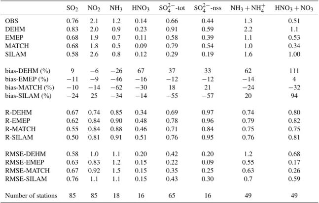
Table 3.Evaluation of modelled air concentrations of sulfur and nitrogen gaseous and aerosol species using observations from the EMEP measurement network (http://www.emep.int) for the years 2000–2010. Unit: µg(S/N)m−3.

SO2 NO2 NH3 HNO3 SO2₄−-tot SO₄2−-nss NH3+NH+₄ HNO₃+NO₃

OBS 0.76 2.1 1.2 0.14 0.66 0.44 1.3 0.51 DEHM 0.83 2.0 0.9 0.23 0.91 0.59 2.2 1.1 EMEP 0.68 1.9 0.7 0.11 0.58 0.39 1.1 0.53 MATCH 0.68 1.8 0.5 0.09 0.79 0.54 1.0 0.34 SILAM 0.58 2.6 0.8 0.12 0.29 0.19 1.6 1.00 bias-DEHM (%) 9 −6 −26 67 37 33 62 111

bias-EMEP (%) −11 −9 −46 −16 −12 −12 −14 4

bias-MATCH (%) −10 −14 −62 −30 18 21 −24 −32

bias-SILAM (%) −24 25 −34 −14 −55 −57 20 94

R-DEHM 0.67 0.74 0.85 0.34 0.69 0.97 0.74 0.80 R-EMEP 0.62 0.84 0.90 0.48 0.78 0.96 0.79 0.82 R-MATCH 0.55 0.84 0.88 0.46 0.71 0.84 0.75 0.75 R-SILAM 0.50 0.81 0.91 0.51 0.76 0.95 0.76 0.81 RMSE-DEHM 0.58 1.0 1.1 0.20 0.42 0.20 1.2 0.68 RMSE-EMEP 0.63 0.83 1.2 0.15 0.22 0.09 0.55 0.17 RMSE-MATCH 0.67 0.92 1.5 0.15 0.35 0.25 0.63 0.26 RMSE-SILAM 0.76 1.1 1.1 0.15 0.43 0.30 0.7 0.59 Number of stations 85 85 18 16 65 16 49 49

Notes: SO2−

4 -tot and SO24−-nss mean total and sea-salt-corrected sulfate respectively.

model’s lowest layer, this being 60 m and 25 m respectively. For the EMEP and MATCH models, 3 m concentrations are estimated from the model’s lowest layer (ca. 45 m grid cen-tre for EMEP, 30 m for MATCH), assuming similarity theory and deposition-induced vertical gradients (Simpson et al., 2012; Robertson et al., 1999).

3.1 Comparison with observations

Observed concentrations of nitrogen and sulfur compounds in air and precipitation were extracted from the EMEP database (http://www.emep.int; Tørseth et al., 2012) for the years 2000–2010. Observed means were constructed for the period, with the criteria of 80 % capture per year over at least 5 yr within this period. For the four CTMs, modelled 20 yr means (1990–2009 climate, 2005 emissions) were con-structed for the measurement sites reaching this criterion. The resulting paired data were evaluated for statistical per-formance using relative bias (%bias), Pearson correlation co-efficient (R) and root-mean-square error (RMSE). The evalu-ation includes air concentrevalu-ations of gaseous and aerosol sul-fur and nitrogen species (Table 3), and deposition and con-centration in precipitation of oxidised sulfur as well as oxi-dised and reduced nitrogen (Table 4). Evaluation of precipi-tation, from ECHAM5 (for DEHM) and from RCA3 (for the three European-scale CTMs), is also included in the evalua-tion (Table 4).

It is important to note that we cannot expect CTM mod-els driven by GCM or RCM meteorology to perform as well as they would with data from NWP models; the latter are the result of assimilating observed data into dedicated me-teorological models. The ECMWF IFS model, for example, continuously assimilates near-surface, airborne and satellite observations to ensure good performance. This NWP model has a spatial resolution of about 16 km, and in standard us-age the EMEP model updates IFS data every 3 h. In contrast, the RCA3 data have a spatial resolution of about 50 km, are updated every 6 h, and have no assimilation of observations. The comparison results presented in Tables 3–4 are thus not designed to reflect optimum model performance but rather to show that, despite the limitations of RCM meteorology, the CTM models still do a reasonable job of reproducing con-centration and deposition levels on a statistical basis.

From Table 3 it is clear that most models do a fair job of capturing SO2and NO2concentrations, but results are mixed

for the other compounds. The reasons for better performance of some compounds compared to others are complex, and not always understood. However, in general we expect better per-formance for “simple” precursors from mainly ground-level sources (e.g. NO2) than from high-level point sources (SO2),

or for compounds with complex chemical pathways and strong deposition-induced gradients, notably HNO3. HNO3

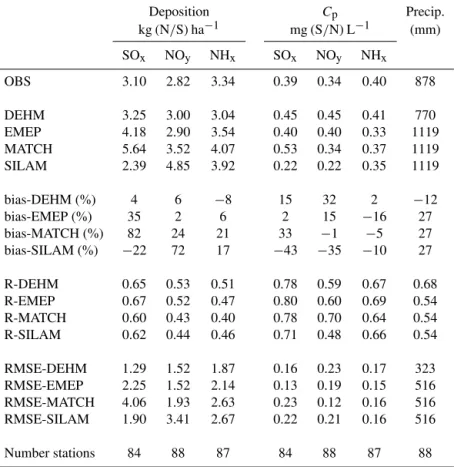
Table 4.Evaluation of modelled wet deposition, concentration in precipitation (Cp) and precipitation using observations from the EMEP

measurement network for the years 2000–2010.

Deposition Cp Precip.

kg(N/S)ha−1 mg(S/N)L−1 (mm)

SOx NOy NHx SOx NOy NHx

OBS 3.10 2.82 3.34 0.39 0.34 0.40 878 DEHM 3.25 3.00 3.04 0.45 0.45 0.41 770 EMEP 4.18 2.90 3.54 0.40 0.40 0.33 1119 MATCH 5.64 3.52 4.07 0.53 0.34 0.37 1119 SILAM 2.39 4.85 3.92 0.22 0.22 0.35 1119 bias-DEHM (%) 4 6 −8 15 32 2 −12

bias-EMEP (%) 35 2 6 2 15 −16 27

bias-MATCH (%) 82 24 21 33 −1 −5 27

bias-SILAM (%) −22 72 17 −43 −35 −10 27

R-DEHM 0.65 0.53 0.51 0.78 0.59 0.67 0.68 R-EMEP 0.67 0.52 0.47 0.80 0.60 0.69 0.54 R-MATCH 0.60 0.43 0.40 0.78 0.70 0.64 0.54 R-SILAM 0.62 0.44 0.46 0.71 0.48 0.66 0.54 RMSE-DEHM 1.29 1.52 1.87 0.16 0.23 0.17 323 RMSE-EMEP 2.25 1.52 2.14 0.13 0.19 0.15 516 RMSE-MATCH 4.06 1.93 2.63 0.23 0.12 0.16 516 RMSE-SILAM 1.90 3.41 2.67 0.22 0.21 0.16 516 Number stations 84 88 87 84 88 87 88

Notes: for any one site, deposition is the product ofCp×Precip, but here we present the averages across

sites of each value.

ammonium nitrate and NH3reactions. The underprediction

of NH3 is, however, expected for all models as the lowest

model layers (between 25 and 90 m thick) will not resolve vertical gradients caused by NH3emissions, and since

mea-surements are often affected by nearby agricultural sources; however EMEP and MATCH show the largest negative bias. The largest discrepancies in the concentrations are seen for some aerosol (or sum of gas+aerosol) components; for ex-ample, both SILAM and DEHM overestimate total nitrate by a factor of 2. For wet deposition (Table 4), results are also mixed, but most results are within 30 %. Regarding wet deposition, we can note that the EMEP network is a mixture of bulk and wet-only collectors, with each country choosing the most appropriate method for its conditions (see http://ebas.nilu.no). For daily sampling, there is not thought to be a large difference in the results in many areas, but with bulk collectors, some dry-deposited material will be incor-rectly assessed as wet deposition. The quality of measure-ment analysis also differs; results for sulfate tend to be some-what better than nitrate, and worse for ammonium measure-ments (EMEP/CCC, 2014). Given these uncertainties (and the use of climate-model-based meteorology), the level of discrepancies seen in Table 4 can be regarded as satisfactory.

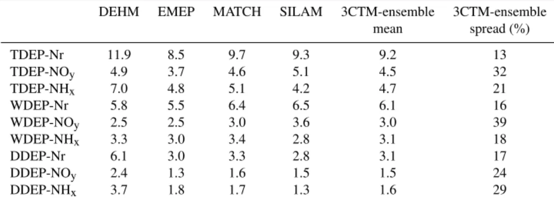
Table 5.Base-case depositions of Nr components (kg(N)ha−1) for the four CTMs, along with the 3CTM-ensemble mean and spread. Values

are average depositions over the EU28+_domain.

DEHM EMEP MATCH SILAM 3CTM-ensemble 3CTM-ensemble mean spread (%) TDEP-Nr 11.9 8.5 9.7 9.3 9.2 13 TDEP-NOy 4.9 3.7 4.6 5.1 4.5 32

TDEP-NHx 7.0 4.8 5.1 4.2 4.7 21

WDEP-Nr 5.8 5.5 6.4 6.5 6.1 16 WDEP-NOy 2.5 2.5 3.0 3.6 3.0 39

WDEP-NHx 3.3 3.0 3.4 2.8 3.1 18

DDEP-Nr 6.1 3.0 3.3 2.8 3.1 17 DDEP-NOy 2.4 1.3 1.6 1.5 1.5 24

DDEP-NHx 3.7 1.8 1.7 1.3 1.6 29 Notes: the 3CTM ensemble consists of the three European-scale CTMs driven by RCA3. Spread is defined as(max−min)/mean of these three models. TDEP, DDEP and WDEP refer to total, dry and wet deposition respectively.

3.2 Deposition maps, base case

Figure 3 presents the results of the four models for total Nr deposition. Patterns of Nr deposition are seen to be generally similar across the four models, with high depositions over the major emission areas in northern Italy and the Benelux area. The DEHM model shows smoother gradients, a result of be-ing driven by the larger scale (and lower resolution) ECHAM meteorological driver. These results are also summarised in Table 5. This table also includes the “3CTM-ensemble” mean and spread, with this small ensemble consisting of the three fine-scale models EMEP, MATCH and SILAM. (DEHM was excluded from the ensemble since its larger scale and lower spatial resolution make its results somewhat different to the RCA3-driven CTMs.) Table 5 shows similar values for the total deposition of Nr from the different mod-els, with a range between 8.5 and 11.9 kg(N)ha−1. The con-tributions from NOyand NHxare almost equal as an

ensem-ble mean, although the models differ somewhat in their rank-ing of these components. The largest differences between the 3CTM-ensemble models and DEHM are seen for the dry-deposition components, with factor of 2 differences. This is likely a result of the lower mixing heights in DEHM dis-cussed in Sect. 3.1 (cf. Supplement, Fig. S3). SILAM shows the highest levels of NOydeposition (especially wet) among

the four CTMs but the lowest deposition of NHx.

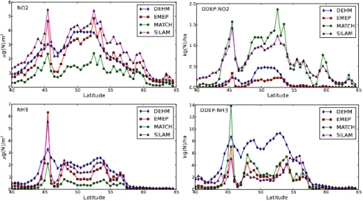
Such differences are not unexpected, as chemical mecha-nisms, deposition process, and dispersion processes are quite different in the four CTMs. As a further illustration of this, Fig. 4 shows concentrations and dry depositions of NO2and

NH3along the north–south European transect at 10◦E

indi-cated in Fig. 1 (this transect was chosen as it passes through many different pollution climates, from the polluted Po Val-ley in the south, through high NH3areas in NW Europe, to

relatively clean areas in the north). Differences are clearly substantial, with, for example, EMEP showing far lower de-position rates of NO2 compared to especially MATCH and

SILAM, despite relatively high NO2 concentrations. This

particular feature likely reflects the EMEP model’s use of lower deposition velocities as a proxy for an NO2

compensa-tion point (this behaviour is switched on when there is no ex-plicit modelling of soil NO emissions). Such model assump-tions can have large impacts on individual species but a lower impact on total Nr concentrations or depositions.

3.3 Scenario runs

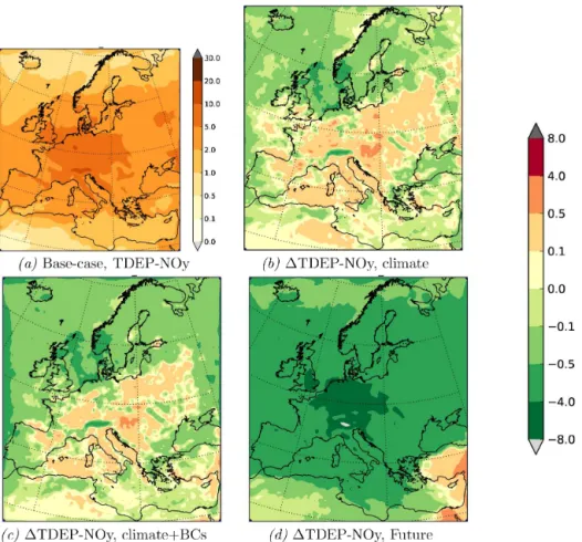
Figure 5a shows the 3CTM-ensemble mean NOydeposition

from the three RCA3-driven European-scale CTMs, with lev-els of around 5–10 kg(N)ha−1_{in central Europe, declining} to less than 2 kg(N)ha−1_{in northern areas. Figure 5b shows} the changes in NOydeposition arising from climate change

only (E05-M00-BC2). Levels of NOy deposition increase

in central Europe to some extent (ca. 0.1–0.5 kg(N)ha−1), but decrease in, for example, the Nordic area by a similar amount. Figure 5c shows the corresponding changes brought about by scenario E05-M50-BC3, in which boundary con-ditions are also allowed to change to 2050 levels, but the picture is little changed from the effects of climate change alone. Figure 5d shows much more dramatic changes in the case of E50-M50-BC3, where European emissions are set to the 2050 levels. NOy deposition is reduced by more than

0.5 kg(N)ha−1 over almost all of Europe, and more than 4 kg(N)ha−1in central areas.

Figure 6 provides similar results for NHxdeposition. The

results of the climate and climate+boundary-conditions sim-ulations are rather similar in magnitude to the equivalent results for NOyspecies, although climate change seems to

increase NHx deposition in northern and eastern regions to

a greater extent than NOy. In broad terms, these

Figure 3.Calculated deposition of total Nr from the four CTMs. Results given as 20 yr means (1990–2009) for the base case (E05-M00-BC1).

Unit: kg(N)ha−1.

Figure 4.Examples of model variability for two compounds. Calculated base-case concentrations (left column, µg(N)m−3) and dry

Figure 5.Results from the 3CTM ensemble (see text), for(a)base-case deposition of NOy(TDEP-NOy, innermost legend), and changes

in TDEP-NOy(rightmost legend) resulting from(b)2050s climate (E05-M50-BC2),(c)2050s climate and boundary conditions

(E05-M50-BC3), and(d)2050s emissions, climate and boundary conditions (E50-M50-BC3). Unit: kg(N)ha−1.

emissions will substantially increase NHxdeposition in large

parts of Europe (discussed further below).

Figure 7 summarises the results of these calculations, pre-senting average depositions over the EU28+_{domain (cf.} Ta-ble 2) from all four models, and four scenarios. As noted above in the spatial maps, the most dramatic changes are only seen with the E50-M50-BC3 scenario, in which emis-sions from the year 2050 are used. Dry and wet deposition of NOydecreases significantly in all models. Dry deposition

of NHxincreases to some extent in all models, whereas wet

deposition of NHxshows smaller changes.

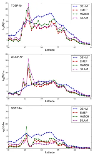
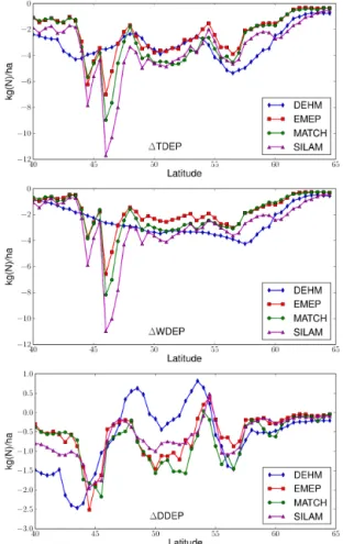
The similarity of results from the three scenarios using 2005 emissions from each model is unsurprising, given that emissions are not changed, and the domain is large, but dif-ferences are much more apparent when looking at smaller regions or particular locations. In order to visualise this bet-ter, Figs. 8 and 9 show the Nr deposition and changes in Nr deposition along the same north–south transect as used in Fig. 4. In Fig. 8, the densely populated (and high-emission, especially for NH3) Italian Po Valley area, starting around

45◦_{N, is clearly visible in the three RCA3-driven CTMs. The} ECHAM5-driven DEHM model shows smoother deposition

patterns, but all models show high Nr deposition from around 45◦_{N to around 58}◦_{N (between Denmark and Norway).} Dif-ferences in Nr deposition are greatest for the dry-deposition components along this transect, with, for example, a factor of 3 between the lowest and highest values in mid-latitudes.

Figure 9 shows the differences between the future case (E50-M50-BC3) and base case for the same components. The models are seen to behave in rather similar ways for total and wet deposition, with substantial reductions (of up to 10 kg(N)ha−1) in the Po Valley region. For dry deposi-tion, the picture is more complex, with larger differences be-tween models, and with some regions experiencing reduced Nr deposition, while others (e.g. around 55◦_{N) experience} increased deposition.

It can be noted that the magnitude and distribution of changes in Nr deposition over Europe is sensitive to the cli-mate projection that is used. Engardt and Langner (2013) compared three different climate projections (including the one used here) using the MATCH model and found changes due to climate change by 2050 of less than ±1 kg(N) ha for both NHy and NHx. These changes are comparable to

D. Simpson et al.: Impacts of climate and emission changes on nitrogen deposition 7007

P

❛♣

❡r

⑤

❉✐s❝✉ss✐♦♥

P

❛♣

❡r

⑤

❉✐s❝✉ss✐♦♥

P

❛♣

❡r

⑤

❉✐s❝

✉ss✐♦♥

P

❛♣

❡r

⑤

Figure 6.Same as Fig. 5 but for reduced nitrogen, NHx.

Figure 7.Calculated deposition components of Nr from four CTMs and four scenarios for the EU28+region. Blocks of bars distinguish wet

Table 6.Excess Nr deposition over 10 kg(N)ha−1yr−1for the four CTMs in the EU28+region.

Model E05-M00-BC1 E05-M50-BC2 E05-M50-BC3 E50-M50-BC3 E50X20-M50-BC3 E50X30-M50-BC3

f₁₀ E₁₀ f₁₀ E₁₀ f₁₀ E₁₀ f₁₀ E₁₀ f₁₀ E₁₀ f₁₀ E₁₀

DEHM 56 3.58 56 3.75 55 3.74 38 2.09 45 3.18 – –

EMEP 37 1.44 38 1.53 37 1.50 19 0.55 28 1.01 32 1.29

MATCH 43 2.41 43 2.44 44 2.46 28 1.04 – – – –

SILAM 40 1.82 39 1.76 39 1.73 18 0.48 – – – –

Notes:f10gives the fraction (%) of EU28+region with Nr depositions in excess of 10 kg(N)ha−1_;E

10gives the mean value of excess deposition (kg(N)ha−1_yr−1_{) averaged}

across the EU28+_region.

Table 7. Statistics of detailed critical load exceedances in the EU28+_{region, EMEP MSC-W model.}

Scenario Area exceeded Mean exceedance

f_CL(%) E_CL(kg(N)ha−1yr−1)

E05-M00-BC1 64.1 3.81 E05-M50-BC2 64.4 3.83 E05-M50-BC3 64.1 3.78 E50-M50-BC3 49.8 1.89 E50X20-M50-BC3 54.9 2.57 E50X30-M50-BC3 56.9 2.94

(2013) reported a general reduction in the Nr deposition over Europe above 0.2 kg(N) ha due to climate change in the period 1990 to 2090 using the hemispheric DEHM model. This could be compared to the case with changing BCs and changing climate in this study, which gives an increase in central/southern Europe for NHyand a more widespread

in-crease for NHx. These differences in results are, however,

small enough to be explained by differences in the climate projection used. Engardt and Langner (2013) also reported changes in Nr deposition due to emission changes until 2050 using the RCP4.5 scenario. The reductions in deposition are comparable to those reported here for NHy, but for NHxthe

distribution of the changes are different, primarily due to dif-ferences in the emission data.

3.4 Changes in NHxpartitioning

Results presented so far have dealt with groups of either ox-idised, reduced or total depositions of Nr compounds. Fig-ure 10 illustrates changes for particular compounds, from one model (EMEP). The oxidised compounds NO, NO2and

nitrate all show relatively straightforward reductions, as ex-pected from the emissions change. PAN is also reduced, but not to the same extent, and PAN also shows more sensi-tivity to the climate and boundary condition changes than other NOy species. The most interesting changes are seen

for the reduced compounds – with substantial increases in gaseous NH3and substantial decreases in particulate

ammo-nium. This effect was also noted by Engardt and Langner (2013) and is caused by the fact that, in the year 2050

sce-Figure 8.Calculated base-case deposition along the 10◦east

tran-sect (cf. Fig. 1), for total Nr deposition (top), wet deposition (mid-dle), dry deposition (bottom).

narios, there is too little sulfate and even too little HNO3to

react with NH3. This effect is further illustrated in Fig. 11,

which shows the changes in (a) NH3deposition and (b) total

NHxdeposition between the base and future case.

Compar-ing these changes to Fig. 2b, it is clear that while the total NHx deposition change is quite similar to that of the

emis-sions, the deposition changes in NH3are clearly much higher

Figure 9.Calculated changes in total, wet and dry deposition of Nr,

future case (E50-M5-BC3) minus base case (E05-M00-BC1). Same transect as Fig. 8.

figure, the sum, NHx, of NH3+NH+₄ is approximately

con-stant from the year 2000s to the 2050s scenario. However, Fig. 10 shows averages over a large area. In fact, as seen in Fig. 11, the deposition of NHx decreases in most parts

of western Europe, especially France, and increases in many parts of central and eastern Europe; see also Fig. 2b for emis-sions. The EU28+ area includes areas in both regimes.)

There are of course many issues with the modelling of ammonia exchange, with clear model limitations associated with the lack of bidirectional exchange in these CTMs (Bash et al., 2013; Flechard et al., 2013; Wichink-Kruit et al., 2010). This will be discussed further in the conclusions. The results of the increased NH3 emissions associated with the

final two scenarios are discussed below in the context of crit-ical load exceedances.

Figure 10.Calculated concentrations of major Nr species from the EMEP MSC-W model for four scenarios. EU28+_region.

4 Exceedances of critical loads

A critical load (CL) is defined as a quantitative estimate of an exposure to one or more pollutants below which signif-icant harmful effects on specified sensitive elements of the environment do not occur according to present knowledge (Nilsson and Grennfelt, 1988). If a deposition is higher than the critical load at a site, the CL is said to be exceeded, and in this paper, exceedances due to total annual N deposition are calculated for the EU28+_{region. Dentener et al. (2006) and} Lamarque et al. (2005) used a fixed, ecosystem-independent CL value of 1 g(N)m−2_yr−1_{(10 kg(N) ha}−1_yr−1_{), as this}

al-lowed comparison across multiple models. Before we con-sider calculations of “real” ecosystem-dependent CL values with the EMEP model, we present first also our multi-model comparison using this simple 10 kg(N) ha−1 _{value. Table 6} compares the area of exceedance of 10 kg(N) ha−1_yr−1_(f

10)

and the average exceedance (E10) for all scenarios used in

this study, including the X20 and X30 variations of the fu-ture case. Table 6 shows that the three European-scale CTMs give similar areas of exceedance of the 10 kg(N) ha−1_yr−1

level (ca. 40 %) in the base case, although MATCH predicts considerably more excess than EMEP. DEHM shows a much larger area of exceedance, and excess, in this case. Similar to results presented above for total depositions, the effect of the E05-M50-BC2 and E05-M50-BC3 scenarios is relatively small. The E50-M50-BC3 scenario shows dramatic reduc-tions inf10andE10compared to the base case.

The DEHM and EMEP models were used for the future scenario with 20 % increased NH3emissions

(E50X20-M50-BC3). Although exceedances are still below the base-case values, the increased NH3has a large impact, with 50 and

80 % increases inE10 compared to the standard future

sce-nario E50-M50-BC3. The EMEP model calculation of the 30 % NH3increase bringsE10values almost back to the 2005

Figure 11.Changes in total deposition (%), from 2005 to 2050, for NH3and NHx. Results from the 3CTM ensemble. The colour scale is

identical to that used for emission changes in Fig. 2.

As noted above, the use of the fixed 10 kg(N)ha−1yr−1 threshold is a simple proxy for CLs. Within the Conven-tion for the Long-range Transboundary Air PolluConven-tion (CLR-TAP, www.unece.org/env/lrtap), for which EMEP provides ecosystem-specific deposition data, CL values are assessed in a much more realistic way. Critical loads are calculated for different receptors (e.g. terrestrial ecosystems, aquatic ecosystems), and “sensitive elements” can be any part (or the whole) of an ecosystem or ecosystem process. Critical loads have been defined for several pollutants (S, N, heavy met-als), but here we restrict ourselves to CLs defined to avoid the eutrophying effects of N deposition (critical load of nu-trient N, CLnut(N)). The CL for a site is either derived

empir-ically or calculated from a simple steady-state mass balance equation(s) that link a chemical criterion (e.g. an acceptable N concentration in soil solution that should not be exceeded) with the corresponding deposition value(s). Methods to com-pute CLs are summarised in the so-called Mapping Manual (UNECE, 2004; De Vries and Posch, 2003).

Values of CLnut(N) are calculated using the current

crit-ical load database held at the Coordination Centre for Ef-fects (CCE; Posch et al., 2011, 2012) and used in support-ing EU and CLRTAP negotiations on emission reductions (Hettelingh et al., 1995, 2001; Reis et al., 2012). The single exceedance number computed for a grid cell (or any other region) is the so-called average accumulated exceedance (AAE), defined as the weighted mean of all ecosystems within the grid, with the weights being the respective ecosys-tem areas (see Posch et al., 2001).

Figure 12 shows the grid AAE values as derived from the EMEP model ecosystem-specific N deposition data for the six scenarios (cf. Table 1). Although reductions in ex-ceedance are especially seen in the E50-M50-BC3 scenario compared to the base case, patterns do not vary dramatically, and there is still widespread exceedance even for this most stringent scenario. To better summarise these scenarios, the

Figure 12.Exceedances of the critical loads for nutrient nitrogen

(CLnut(N)) in the EU28+region, EMEP MSC-W model, for the six

Figure 13.Inverse cumulative distribution functions of exceedances

(AAE) of CLnut(N) in EU28+for the six scenarios using the EMEP

MSC-W model. Note that scenarios 2 and 3 (black thin lines) barely differ from the base scenario.

inverse cumulative distribution functions of the exceedances are shown in Fig. 13. Exceedances for the three scenarios dis-tinguished only by meteorology and/or boundary condition are similar (see also Table 7 for some statistics), whereas the change in emissions has clearly the largest overall impact. Exceedance levels for the X20 and X30 versions of the 2050 scenarios are well below the scenarios representative of the 2000s but substantially greater than the E50-M50-BC3 case.

5 Conclusions

This study has compared predictions of nitrogen deposition from four chemical transport models (CTMs) for both current conditions and future scenarios. All models were driven by the same basic emission system (except for biogenic VOC, which was model-specific). The three European-scale CTM models were driven by the same regional climate model (RCA3) meteorology, and also by a common set of bound-ary conditions given by the fourth (hemispheric-scale) CTM, DEHM. One base case and three main scenario cases were designed to explore the impact of climate, boundary condi-tions and emissions changes on European N deposition. Two further speculative scenarios were also explored with 1–2 models.

As all of these models have been driven by data from global and/or regional climate models, rather than “real” NWP meteorology, it is not possible to directly compare to measurements. However, we have compared modelled and observed data in a statistical way, and in general the model results seem comparable to the observations (most compo-nents were predicted within 30 %). Some significant discrep-ancies were found, which in the case of the DEHM model could be ascribed to problems caused by the large-scale cli-mate data that are not normally seen in typical DEHM usage.

Deposition estimates from the models were compared as large-scale average, and illustrated for a north–south transect. Although modelled total deposition was rather similar among the models (presumably reflecting prescribed emissions), dif-ferences for wet or dry contributions were typically of the order of 30 %. For specific locations (as illustrated along our transect), or even more so for specific compounds, differ-ences can be much greater. Of course, such differdiffer-ences are not unexpected since many aspects of Nr modelling are not well constrained. For example, there is a lack of data which could specify the proper partitioning of NOybetween HNO3

and fine or coarse nitrate. Further, large variability in dry-deposition rates (with factors of 2–3) is known to exist among deposition modules (Flechard et al., 2011). This variability is a reflection of the difficulties in measuring deposition rates (e.g. Fowler et al., 2009; Pryor et al., 2008) and also of com-plications due to bidirectional fluxes (discussed below) and chemical interactions. There is thus a lack of data with which to constrain dry-deposition fluxes, and this is reflected in the differences in modelled Nr depositions found in this study.

Other results from the model comparison can be sum-marised:

– All models clearly show that the impact of emissions changes is much greater than the impact of climate change alone, or of both climate change and emissions changes outside of Europe.

– The biggest difference between the models is for pre-dictions of individual N compounds. Prepre-dictions for wet and total deposition were, however, broadly consis-tent, although the three fine-scale models resolve Euro-pean emission areas and spatial changes better than the hemispheric-scale model.

– The model predictions for 2050 generally follow the emission changes, with significant reductions in oxi-dised N concentrations and depositions, but slightly in-creasing levels of reduced N deposition.

– For reduced nitrogen, the 2050 emissions are predicted to cause a large increase in gaseous NH3deposition in

most of Europe, but with large corresponding decreases in ammonium. This difference is caused by the much re-duced levels of both SO2and HNO3in the future

atmo-sphere, preventing the formation of ammonium sulfates or nitrates.

(mean exceedance of 1.89 kg(N)ha−1yr−1, down from 3.81 kg(N)ha−1_yr−1_{in the base case).}

– Two further scenarios were explored, involving 20 and 30 % increases in NH3emissions above expected 2050

levels, which reflects the possibility that the emission rates might respond to climate change more than ac-counted for in the emissions inventory. Comparison of these runs against the CL data shows that even a 30 % increase in NH3 will not bring exceedances back to

2000s levels, but such climate-induced increases cause CL exceedances that are substantially larger than those of the standard 2050 emission scenario (worst case here 57 % of areas in excess, with 2.9 kg(N)ha−1yr−1mean exceedance).

Major problems remain in predicting NH3deposition in

particular. With regard to emissions control strategies, the in-creased NH3 deposition noted above (and in, for example,

Engardt and Langner, 2013) implies that local control mea-sures might become more effective. On the other hand, En-gardt and Langner (2013) also estimated longer lifetimes of S and NHycompounds in the future, thus increasing the

in-ternational transport of some particles. Wichink-Kruit et al. (2012) also showed that inclusion of bidirectional exchange increases the transport distance of NHx, which would affect

any predictions of Nr deposition and CL exceedance. Indeed, the complexities of bidirectional exchange have been noted in many papers (e.g. Sutton et al., 1995; Nemitz and Sutton, 2004; Fowler et al., 2009; Massad et al., 2010; Flechard et al., 2013), and some CTMs have attempted to include such ex-change (e.g. Wichink-Kruit et al., 2010; Bash et al., 2013). However, such modelling is limited by many factors, includ-ing process uncertainties (Massad et al., 2010; Flechard et al., 2013), problems of sub-grid heterogeneity (e.g. Loubet et al., 2001, 2009) and lack of necessary and accurate input data.

Still, the overriding conclusion of this paper is probably robust: reducing future deposition of Nr in Europe is mainly dependent upon the way in which future NH3emissions

de-velop. The new recognition that climate change may influ-ence emissions much more than currently accounted for in official inventories makes it even more important that meth-ods to deal with NH3emissions are improved.

The Supplement related to this article is available online at doi:10.5194/acp-14-6995-2014-supplement.

Acknowledgements. This study was initiated and mainly

supported by the Nordic Council of Ministers (EnsCLIM project, NMR no. KoL-10-04) and the EU project ECLAIRE (project no. 282910). Further support came from the EU projects MEGAPOLI (no. 212520), PEGASOS (no. 265148), TRANSPHORM (no. 243406), NMR FAN (kol-1204) and Danish

ECOCLIM projects, and the Swedish Environmental Protection Agency through the research programme CLEO (Climate Change and Environmental Objectives) as well as EMEP under the LRTAP UNECE Convention. The work is also a contribution to the Swedish Strategic Research Areas Modelling the Regional and Global Earth System (MERGE). Thanks are due to C. Heyes and Z. Klimont at IIASA for valuable help with the emission inventory processing. Edited by: E. Nemitz

References

Aas, W., Tsyro, S., Bieber, E., Bergström, R., Ceburnis, D., Eller-mann, T., Fagerli, H., Frölich, M., Gehrig, R., Makkonen, U., Nemitz, E., Otjes, R., Perez, N., Perrino, C., Prévôt, A. S. H., Putaud, J.-P., Simpson, D., Spindler, G., Vana, M., and Yt-tri, K. E.: Lessons learnt from the first EMEP intensive measurement periods, Atmos. Chem. Phys., 12, 8073–8094, doi:10.5194/acp-12-8073-2012, 2012.

Amann, M., Klimont, Z., and Wagner, F.: Regional and global emissions of air pollutants: recent trends and future scenar-ios, Annu. Rev. Env. Resour., 38, 31–55, doi:10.1146/annurev-environ-052912-173303, 2013.

Amann, M., Borken-Kleefeld, J., Cofala, J., Heyes, C., Klimont, Z., Rafaj, P., Purohit, P., Schoepp, W., and Winiwarter, W.: Future emissions of air pollutants in Europe – Current leg-islation baseline and the scope for further reductions, TSAP Report #1, Institute for Applied Systems Analysis (IIASA), Laxenburg, Austria, http://webarchive.iiasa.ac.at/Admin/PUB/ Documents/XO-12-011.pdf, 2012.

Andersson, C. and Engardt, M.: European ozone in a fu-ture climate: importance of changes in dry deposition and isoprene emissions, J. Geophys. Res., 115, D02303, doi:10.1029/2008JD011690, 2010.

Andersson, C., Langner, J., and Bergstrom, R.: Interannual variation and trends in air pollution over Europe due to climate variabil-ity during 1958-2001 simulated with a regional CTM coupled to the ERA40 reanalysis, Tellus B, 59, 77–98, doi:10.1111/j.1600-0889.2006.00196.x, 2007.

Asman, W. A. H., Sørensen, L. L., Berkowicz, R., Granby, K., Nielsen, H., Jensen, B., Runge, E., Lykkelund, C., Gryning, S. E., and Sempreviva, A. M.: Dry deposition processes, Danish En-vironmental Protection Agency, Marine Research, 35, Copen-hagen, Denmark, 1994.

Bash, J. O., Cooter, E. J., Dennis, R. L., Walker, J. T., and Pleim, J. E.: Evaluation of a regional air-quality model with bidi-rectional NH3 exchange coupled to an agroecosystem model,

Biogeosciences, 10, 1635–1645, doi:10.5194/bg-10-1635-2013, 2013.

Binkowski, F. and Shankar, U.: The Regional Particulate Matter Model, 1. Model description and preliminary results, J. Geophys. Res., 100, 26191–26209, 1995.

intercontinen-tal transport of air pollution, Atmos. Environ., 53, 156–176, doi:10.1016/j.atmosenv.2012.01.011, 2012.

Christensen, J. H.: The Danish Eulerian Hemispheric Model – a three-dimensional air pollution model used for the Arctic, At-mos. Environ., 31, 4169–4191, 1997.

Colette, A., Granier, C., Hodnebrog, Ø., Jakobs, H., Maur-izi, A., Nyiri, A., Bessagnet, B., D’Angiola, A., D’Isidoro, M., Gauss, M., Meleux, F., Memmesheimer, M., Mieville, A., Rouïl, L., Russo, F., Solberg, S., Stordal, F., and Tampieri, F.: Air quality trends in Europe over the past decade: a first multi-model assessment, Atmos. Chem. Phys., 11, 11657–11678, doi:10.5194/acp-11-11657-2011, 2011.

Colette, A., Granier, C., Hodnebrog, Ø., Jakobs, H., Mau-rizi, A., Nyiri, A., Rao, S., Amann, M., Bessagnet, B., D’Angiola, A., Gauss, M., Heyes, C., Klimont, Z., Meleux, F., Memmesheimer, M., Mieville, A., Rouïl, L., Russo, F., Schucht, S., Simpson, D., Stordal, F., Tampieri, F., and Vrac, M.: Future air quality in Europe: a multi-model assessment of pro-jected exposure to ozone, Atmos. Chem. Phys., 12, 10613– 10630, doi:10.5194/acp-12-10613-2012, 2012.

Cuvelier, C., Thunis, P., Vautard, R., Amann, M., Bessagnet, B., Bedogni, M., Berkowicz, R., Brandt, J., Brocheton, F., Built-jes, P., Carnavale, C., Coppalle, A., Denby, B., Douros, J., Graf, A., Hellmuth, O., Hodzic, A., Honore, C., Jonson, J., Kerschbaumer, A., de Leeuw, F., Minguzzi, E., Moussiopou-los, N., Pertot, C., Peuch, V., Pirovano, G., Rouil, L., Sauter, F., Schaap, M., Stern, R., Tarrason, L., Vignati, E., Volta, M., White, L., Wind, P., and Zuber, A.: CityDelta: a model inter-comparison study to explore the impact of emission reductions in European cities in 2010, Atmos. Environ., 41, 189–207, 2007. Dentener, F., Drevet, J., Lamarque, J. F., Bey, I., Eickhout, B., Fiore, A. M., Hauglustaine, D., Horowitz, L. W., Krol, M., Kulshrestha, U. C., Lawrence, M., Galy-Lacaux, C., Rast, S., Shindell, D., Stevenson, D., Van Noije, T., Atherton, C., Bell, N., Bergman, D., Butler, T., Cofala, J., Collins, B., Do-herty, R., Ellingsen, K., Galloway, J., Gauss, M., Montanaro, V., Mueller, J. F., Pitari, G., Rodriguez, J., Sanderson, M., Sol-mon, F., Strahan, S., Schultz, M., Sudo, K., Szopa, S., and Wild, O.: Nitrogen and sulfur deposition on regional and global scales: a multimodel evaluation, Global Biogeochem. Cy., 20, GB4003, doi:10.1029/2005GB002672, 2006.

De Vries, W. and Posch, M.: Critical levels and critical loads as a tool for air quality management, in: Handbook of Atmospheric Science – Principles and Applications, edited by: Hewitt, C. N. and Jackson, A. V., chap. 20, Blackwell Science, Oxford, UK, 562–602, 2003.

Dore, A., Carslaw, D., Chemel, C., Derwent, R., Fisher, B., Grif-fiths, S., Lawrence, S., Metcalfe, S., Redington, A., Simpson, D., Sokhi, R., Sutton, P., Vieno, M., and Whyatt, J.: Evaluation and inter-comparison of acid deposition models for the UK, in: Air Pollution Modelling and its Application XXII, edited by: Steyn, D., Builtjes, P., and Timmermans, R., NATO Science for Peace and Security Series C. Environmental Security, Springer, Dordrecht, 32nd NATO/SPS International Technical Meeting, 505–509, 2013.

Emberson, L., Simpson, D., Tuovinen, J.-P., Ashmore, M., and Cambridge, H.: Towards a model of ozone deposition and stom-atal uptake over Europe, EMEP MSC-W Note 6/2000, The Nor-wegian Meteorological Institute, Oslo, Norway, 2000a.

Emberson, L., Wieser, G., and Ashmore, M.: Modelling of stomatal conductance and ozone flux of Norway spruce: comparison with field data, Environ. Pollut., 109, 393–402, 2000b.

Emberson, L., Ashmore, M., Simpson, D., Tuovinen, J.-P., and Cambridge, H.: Modelling and mapping ozone deposition in Eu-rope, Water Air Soil Pollut., 130, 577–582, 2001.

Emberson, L. D., Büker, P., and Ashmore, M. R.: Assessing the risk caused by ground level ozone to European forest trees: a case study in pine, beech and oak across different climate regions, En-viron. Pollut., 147, 454–466, doi:10.1016/j.envpol.2006.10.026, 2007.

EMEP/CCC: Results from EMEP laboratory intercomparison, EMEP/CCC results on web, The Norwegian Institute for Air Research (NILU), Kjeller, Norway, http://www.nilu.no/projects/ ccc/intercomparison/index.html, 2014.

Engardt, M.: Sulphur simulations for East Asia using the MATCH model with meteorological data from ECMWF, RMK 88, Swedish Meteorological and Hydrological Institute, 33 pp., 2000.

Engardt, M. and Langner, J.: Simulations of future sulphur and nitrogen deposition over Europe using meteorological data from three regional climate projections, Tellus B, 65, 20348, doi:10.3402/tellusb.v65i0.20348, 2013.

Erisman, J. W., Hensen, A., Fowler, D., Flechard, C. R., Grüner, A., Spindler, G., Duyzer, J. H., Weststrate, H., Römer, F., Vonk, A. W., and Jaarsveld, H. V.: Dry deposition monitoring in Europe, Water Air Soil Pollut., 1, 17–27, 2001.

Erisman, J. W., Galloway, J. N., Seitzinger, S., Bleeker, A., Dise, N. B., Petrescu, A. M. R., Leach, A. M., and de Vries, W.: Consequences of human modification of the global nitro-gen cycle, Philos.Trans. R. Soc. Lond. B. Biol. Sci., 368, doi:10.1098/rstb.2013.0116, 2013.

Fagerli, H. and Aas, W.: Trends of nitrogen in air and precipitation: model results and observations at EMEP sites in Europe, 1980– 2003, Environ. Pollut., 154, 448–461, 2008.

Finlayson-Pitts, B. and Pitts, J.: Chemistry of the Upper and Lower Atmosphere – Theory, Experiments, and Applications, Aca-demic Press, San Diego, CA, USA, 2000.

Flechard, C. R., Nemitz, E., Smith, R. I., Fowler, D., Ver-meulen, A. T., Bleeker, A., Erisman, J. W., Simpson, D., Zhang, L., Tang, Y. S., and Sutton, M. A.: Dry deposition of reactive nitrogen to European ecosystems: a comparison of in-ferential models across the NitroEurope network, Atmos. Chem. Phys., 11, 2703–2728, doi:10.5194/acp-11-2703-2011, 2011. Flechard, C. R., Massad, R.-S., Loubet, B., Personne, E.,

Simp-son, D., Bash, J. O., Cooter, E. J., Nemitz, E., and Sutton, M. A.: Advances in understanding, models and parameterizations of biosphere-atmosphere ammonia exchange, Biogeosciences, 10, 5183–5225, doi:10.5194/bg-10-5183-2013, 2013.

Forkel, R. and Knoche, R.: Nested regional climate-chemistry simulations for central Europe, C. R. Geosci., 339, 734–746, doi:10.1016/j.crte.2007.09.018, 2007.