www.hydrol-earth-syst-sci.net/19/3301/2015/ doi:10.5194/hess-19-3301-2015
© Author(s) 2015. CC Attribution 3.0 License.
Complex network theory, streamflow, and hydrometric monitoring
system design
M. J. Halverson1,2and S. W. Fleming2,1,3
1Department of Earth, Ocean, and Atmospheric Sciences, University of British Columbia, Vancouver, BC, Canada 2Science Division, Meteorological Service of Canada, Environment Canada, Vancouver, BC, Canada
3College of Earth, Ocean, and Atmospheric Sciences, Oregon State University, Corvallis, Oregon, USA
Correspondence to:M. J. Halverson ([email protected])
Received: 25 October 2014 – Published in Hydrol. Earth Syst. Sci. Discuss.: 15 December 2014 Revised: 30 May 2015 – Accepted: 1 June 2015 – Published: 31 July 2015
Abstract. Network theory is applied to an array of stream-flow gauges located in the Coast Mountains of British Columbia (BC) and Yukon, Canada. The goal of the analy-sis is to assess whether insights from this branch of math-ematical graph theory can be meaningfully applied to hy-drometric data, and, more specifically, whether it may help guide decisions concerning stream gauge placement so that the full complexity of the regional hydrology is efficiently captured. The streamflow data, when represented as a com-plex network, have a global clustering coefficient and av-erage shortest path length consistent with small-world net-works, which are a class of stable and efficient networks common in nature, but the observed degree distribution did not clearly indicate a scale-free network. Stability helps en-sure that the network is robust to the loss of nodes; in the context of a streamflow network, stability is interpreted as insensitivity to station removal at random. Community struc-ture is also evident in the streamflow network. A network theoretic community detection algorithm identified separate communities, each of which appears to be defined by the combination of its median seasonal flow regime (pluvial, ni-val, hybrid, or glacial, which in this region in turn mainly reflects basin elevation) and geographic proximity to other communities (reflecting shared or different daily meteoro-logical forcing). Furthermore, betweenness analyses suggest a handful of key stations which serve as bridges between communities and might be highly valued. We propose that an idealized sampling network should sample high-betweenness stations, small-membership communities which are by defi-nition rare or undersampled relative to other communities, and index stations having large numbers of intracommunity
links, while retaining some degree of redundancy to maintain network robustness.
1 Introduction 1.1 Network theory
Network theory is the practical application of graph theory, which is itself the study of the structures formed by a system of pairwise relationships (Elsner et al., 2009). In this paper we will use the terms network theory and graph theory inter-changeably. The system in this context consists of a collec-tion of nodes (vertices in graph theory), which are connected to each other by links (edges). Such a general and simple con-cept has allowed a wide range of systems to be successfully studied with graph theory. Network theory has been applied to a tremendous variety of systems, such as social networks, communication networks (e.g., the Internet), transportation networks (e.g., airports), epidemiology, ecology, climate, and biomolecular networks. Overviews of network theory and its real-world applications are provided by, for example, Stro-gatz (2001), Tsonis et al. (2006), Newman (2008), da Fon-toura Costa et al. (2011), and Sen and Chakrabarti (2013). 1.2 Definitions
particu-larly useful because they allow the network under considera-tion to be easily compared to known network types, which have well-known characteristics. Expressions for some of these metrics can be written in more than one way, and cer-tain formulations can be highly geometric in character. For practical applications, these definitions are most commonly phrased as follows (e.g., da Fontoura Costa et al., 2007; Sen and Chakrabarti, 2013). Consider a network containing N nodes. Begin by defining the N×N adjacency matrix,aij,
which is 1 if nodes iandj are connected and 0 otherwise; entries along the diagonal are 0 by convention, unless the network contains self-loops, a concept we will not explore here. The degree, k, of a given node is the number of other nodes to which it is connected, that is, the number of links the node possesses. The degree of node ican be expressed in terms of the adjacency matrix aski=Paij∀j. Then, the
degree distribution, P (k), is the probability distribution of network degrees across all the nodes, i=1,N, in the net-work. The other two metrics,C andL, are scalar quantities. The clustering coefficient measures the tendency for nodes to cluster together into so-called cliques. The neighbourhood of a given node is normally defined to be the set of nodes to which it is linked. Thus, we can represent the neighbour-hood of the ith node asj|aij=1. Then, the local
cluster-ing coefficient for that node is the number of links amongst the nodes in its neighbourhood, expressed as a proportion of the maximum number of links possible amongst the bouring nodes, that is, the probability that the direct neigh-bours of a given node are themselves direct neighneigh-bours. The clustering coefficient for theith node can be represented as Ci=[ki(ki−1)]−12E, whereEis the number of links that
are actually observed to exist between the k neighbours of nodei. We follow standard practice and use the average of all the local clustering coefficients over the network as a bulk measure of the clustering tendency or cliquishness of the net-work as a whole. Finally, average path length is the average over all nodes of the shortest path,dij, between every
combi-nation of node pairs. Path length is measured as the number of links needed to connect a node pair. Thus, the average path length is given asL=[N (N−1)]−1Pdij∀i6=j.
The application of these three fundamental graph theoreti-cal measures to real networks has revealed the existence of a diverse range of network topologies (e.g., Tsonis et al., 2006; da Fontoura Costa et al., 2011; Sen and Chakrabarti, 2013). However, many fall within a small number of known archi-tectures. This library of topologies is widely used across the physical and social sciences to characterize, classify, and un-derstand networks.
The simplest network is a regular network, where, by def-inition, each node has the same number of degrees. A simple example is a 3-D Cartesian grid. In the special case where each node is connected to every other node, the network is said to be fully connected. Regular networks display a wide range of properties because there are many ways to construct them while keeping the degree uniform across all nodes.
In general, however, regular networks are highly clustered, and therefore said to be stable, but have long average path lengths, implying inefficiency. In the context of complex net-works, stability means that the removal of any randomly cho-sen node will have little effect on the network as a whole, while efficiency means that information may easily be prop-agated across the network because the average path length is small. Another fundamental type is the random network. Random networks are networks whereby pairs of nodes are connected randomly. Random networks have a small cluster-ing coefficient and a small average path length, which means that they tend to be unstable but efficient.
While regular and random networks serve as useful ide-alizations, they are not often observed in real-world phe-nomena. Instead, the so-called “small-world” network has been found to describe a number of networks found in nature and engineering. Small-world networks are regarded as a hy-brid of random and regular networks because they are highly clustered (like regular graphs) and have short path lengths (like random graphs) (Watts and Strogatz, 1998). They are said to be both stable and efficient. Examples of small-world networks include the climate system (Tsonis and Roebber, 2004), social networks (i.e., the six degrees of separation phenomenon), and the power grid of the western United States. The small-world classification does not necessarily specify the degree distribution.
One subset of small-world networks, known as scale-free, has been particularly successful in describing real systems. The degree distribution for these networks asymptotes to a power law relationship for large k, that is, P (k)∝k−γ, meaning nodes with a large number of degrees are present but rare. These networks retain the stability and efficiency of small-world networks. However, their outstanding char-acteristic is that they contain supernodes, which are rare but important nodes that contain a very high number of degrees. The climate and Internet networks are examples of small-world networks which are also scale-free.
1.3 Application to hydrometric networks
net-work topologies. In doing so, minor analytical or interpre-tive adjustments from prior applications of network theory need to be considered, as discussed in due course below. The overall notion, however, is straightforward in principle: we test the idea that stream gauges constitute nodes in a formal graph theoretic construct as described generically above, and the relationships between the flow time series measured at each such station form the links.
Our second goal is to assess whether these network theo-retic results might inform the optimal design of hydrometric monitoring systems. As network theory describes the com-plex relationships between a system of measurement points – in our case, hydrometric stations – it seems reasonable to conjecture that certain outcomes from this theory might con-tain insight that could be useful in hydrometric monitoring system design. Because our implementation of network the-ory is based on historically observed hydrologic time series, this information would take the form of guidance on deciding which existing stations are most important, least important, or important in various different respects. More specifically, the results might be used to guide decisions about the place-ment or removal of gauges within the region while retaining the maximum amount of information. In other words, our analysis helps address questions such as the following: what is the degree of redundancy in the current network? Are there under-sampled regions? Is the network, in its current state, stable and efficient?
The study is conducted within the geographic context of the Coast Mountains of British Columbia and Yukon. As discussed in more detail below, this region, which spans al-most 2000 km along the Pacific coast of Canada and adjacent interior regions, exhibits a distinctive range of streamflow regimes. It receives high annually averaged precipitation, and the extreme vertical relief, exceeding 4000 m over short dis-tances, lends itself to microclimates and complicated hydro-logic dynamics which are strongly varied in both space and time. Both the forest and glacial hydrology of the region, for example, are highly complex and remain incompletely un-derstood. Furthermore, using stream gauges to capture such complexity over a large swath of difficult terrain is challeng-ing, especially under the constraint of a finite operating bud-get and logistical challenges associated with establishing and maintaining gauging stations, so that any additional guiding information regarding sampling system design may be use-ful.
The work presented here has some practical limitations which should be recognized. As a first-of-its-kind investi-gation, we elect to maintain simplicity in certain aspects of the analysis. Earth science applications of network theory are growing rapidly, but remain in their relative infancy. The pre-ponderance of these applications appears to focus on global climate dynamics (Tsonis and Roebber, 2004; Yamasaki et al., 2008; Donges et al., 2009; Martin et al., 2013), with some other examples including studies of hurricanes and earth-quakes (e.g., Elsner et al., 2009; Fogarty et al., 2009; Abe
and Suzuki, 2004). For a recent review of geoscientific ap-plications of graph theory, see Phillips et al. (2015). Nar-rowing the view to water resource studies, network theory applications have been even more limited to date, though evidently valuable to the extent that they have been con-ducted. Examples appear to include analysis of virtual wa-ter trade networks, river network analysis, hydrologic con-nectivity analysis, and exploration of new hydrologic mod-elling paradigms (Rinaldo et al., 2006; Suweis et al., 2011; Spence and Phillips, 2014; Sivakumar, 2015). To our knowl-edge, only one other study has performed a quantitative net-work theoretic analysis of observational streamflow data, an innovative study primarily involving application of a modi-fied clustering coefficient to a large assemblage of stream-flow stations spanning the coterminous US (Sivakumar and Woldemeskel, 2014). Furthermore, no prior work has eval-uated which of the fundamental network architectures dis-cussed above (small-world, scale-free, and so forth) best de-scribes the dynamics of streamflow; or employed the com-munity detection algorithms associated with network theory, as discussed in more detail below, for studying river dis-charge; or used any of these techniques for informing the optimal design of streamflow monitoring systems. In light of this, we obviously cannot provide a comprehensive and com-parative study of all such possible applications, and we are obligated to somewhat restrict our scope, such as our choice of focusing strictly on daily flows for a particular region.
and Coulibaly, 2014). A review specifically of streamflow monitoring system design applications of such methods is provided by Mishra and Coulibaly (2009), and for a recent example of continued innovation in this field, see Hannaford et al. (2013). The network theoretic approach implemented here adds to this rich heritage. However, it is far beyond the scope of the present study to compare this method to the data analysis-based techniques for informing the hydromet-ric monitoring system design listed above; nor do we claim that it is superior (or in fact that any single method should be viewed as such). Perhaps more importantly, we empha-size that like these other techniques, the network theoretic approach appears restricted to providing information about the relative importance of previously operated gauges, giv-ing less direct insight into the optimal placement of new gauges, and not explicitly incorporating important types of non-technical considerations into sampling system design.
With this in mind, our results confirm that network the-ory can indeed be successfully used to describe inter-gauge hydrologic relationships, and to guide sampling system de-sign in a novel way which seems fruitful and warrants fur-ther investigation by the hydrologic community. The results additionally add to the broader literature in network theory by quantitatively identifying the network properties and, in particular, the fundamental network topology associated with the terrestrial hydrologic cycle.
2 Study area and data
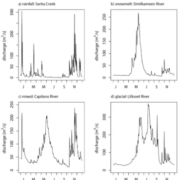
In general, streamflow is determined by the interaction of weather and climate with the terrestrial environment. The specific factors which determine the nature of observed daily streamflows (i.e., the hydrograph) in the Coast Mountains are numerous. The region consists primarily of temperate rain forest, but also includes extensive glaciated alpine areas and some drier inland locations. The broad meteorological context involves the progression of a series of North Pacific frontal storms propagating roughly eastward across the re-gion over the November-to-March storm season, occasion-ally with warmer tropical or sub-tropical moisture feeds as-sociated with atmospheric rivers. Generally drier conditions prevail during the summer. The first-order controls on local terrestrial hydrologic responses to this meteorological forc-ing are drainage elevation and drainage area, which can be viewed as gross descriptors incorporating or parameterizing a number of complex characteristics and processes (precip-itation type, ice cover, forest cover, groundwater, soil mois-ture, storage, and so forth). Drainages in the Coast Mountains exhibit a wide range in mean basin elevation and drainage area, which in turn creates a variety of hydrograph types. Broadly speaking, however, streamflow hydrographs in the Coast Mountains can be classified by their dominant fresh-water source: rainfall, snowmelt, and glacier melt (e.g., Eaton and Moore, 2010).
Figure 1.Selected examples illustrating the four main types of
an-nual hydrographs found in the Coast Mountains of British Columbia and Yukon as described by Eaton and Moore (2010).
Daily discharge data for all of Canada are maintained and archived by the Water Survey of Canada. In this study, only stations with continuous daily discharge records were se-lected, and geographic range was constrained to stations on rivers originating in the Coast Mountains (Fig. 2). We re-stricted the station search to select only natural drainages, omitting rivers regulated by dams or other structures. We ad-ditionally screened for record completeness, requiring each station to have more than 80 % of the possible daily values. The longest daily record dates back to 1903, but the total number of stations in the database steadily increases with time over the 100+years. Therefore, to maximize the num-ber of stations in the analysis, the period 2000–2009 was se-lected because it contained the highest number of active sta-tions. This choice involves a trade-off. A 10-year record is in-sufficient to analyze climatic effects. For example, El Niño– Southern Oscillation, the Pacific Decadal Oscillation, and the Arctic Oscillation impact the hydrology of the Coast Range in British Columbia (BC) and Yukon, and some of those ef-fects differ between regime types (Fleming et al., 2006, 2007; Whitfield et al., 2010). Likewise, longer-term climatic trends may affect different hydrologic regime types within the re-gion in different ways or, eventually, lead to regime transi-tions from one type to another (Whitfield et al., 2002; Flem-ing and Clarke, 2003; Stahl and Moore, 2006; Schnorbus et al., 2014). Thus, distinctions between the lower-frequency hydroclimatic dynamics of different stations seem unlikely to be fully captured by the present analysis. The reward gained in exchange for this sacrifice is maximization of the num-ber of stream gauges incorporated into the analysis. As the density of stream gauges is extremely sparse through much of our study area (e.g., Whitfield and Spence, 2011; Mor-rison et al., 2012), and analysis of climatic effects is merely one of the many uses of hydrologic monitoring networks (see Sect. 1), our choice is reasonable for our current purposes.
A total of 127 stations met the selection criteria. The tribution of stations primarily reflects the population dis-tribution, meaning that the greatest density of stations is found near the dense urban centres of southwestern British Columbia. Drainage elevation statistics were computed by constructing a digital elevation model (DEM) for each gauged basin. Gridded tiles from three DEM products were used: the 25 m British Columbia Terrain Resource Informa-tion Management (TRIM), the 30 m USGS NaInforma-tional Eleva-tion Database, and the 30 m Yukon DEM. Mean elevaEleva-tion was calculated as the average of all cells for each gauge basin using the ESRI ArcGIS Arc/Info and Spatial Ana-lyst/GRID software. Mean drainage elevation ranges from 127 to 2252 m, with an average of 1186 m, while drainage areas range from 2.9 to 50 900 km2, with a median value of 318 km2.
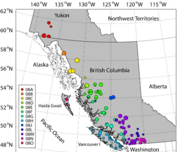
Figure 2.Map of the Canadian west coast showing the 127 Water
Survey of Canada (WSC) streamflow gauging stations used in this study. The stations are coloured according to the first three charac-ters in the WSC naming convention (example – 08M), which defines the stations according to subdivisions of the major drainage basins. The size of each circle scales with the logarithm of the drainage area. The streamflow database was subsetted for stations draining the Coast Mountains.
3 Network topology 3.1 Link definition
In some applications of network theory, the decision of whether to assign a link to a pair of nodes is straightforward. For example, in a social network, friendships define the links between people. In the case of the Internet, websites can be unambiguously connected by hyperlinks. In other applica-tions, there might not be a straightforward binary relation-ship between nodes, meaning it becomes necessary to con-sider empirical relationships. A simple and common method is to assign links to node pairs which share a linear (Pear-son) correlation coefficient,rp, which exceeds some
thresh-old,rt. Such an approach has been extensively used in
stud-ies of the global climate system (e.g., Tsonis and Roebber, 2004; Donges et al., 2009; Yamasaki et al., 2008), as well as in finance and genetics (see references in Tsonis et al., 2011). Numerous other methods for defining links have been developed (e.g., Abe and Suzuki, 2004; Elsner et al., 2009; Fogarty et al., 2009), but they are, to some degree, specific to the data set and scientific objective.
If links are defined by a threshold correlation coefficient, then the question of which threshold to choose naturally arises. A few specific methods have been explored in prior studies. Here, we usert=0.7 because it is intuitively and
about 50 % or more of the variance in the other. Note that this value is generally similar to the ranges considered by Sivaku-mar and Woldemeskel (2014) in their analysis of streamflow data, and by various climate studies using correlation-based network link definitions (e.g., Tsonis and Swanson, 2008).
When calculating the correlation matrix, a pairwise-complete method was chosen to avoid the errors that could otherwise be introduced by interpolating over missing data. The correlation matrix is then thresholded atrtto form an
ad-jacency matrix,aij. As noted in the introductory section, this
is a matrix consisting of logical elements that define which node pairs are linked. The network analysis was carried out using theigraphpackage (Csardi and Nepusz, 2006) in the GNU Rcomputing environment (R Core Team, 2014).
3.2 Inferred network type
The network formed by the 127 streamflow records dis-tributed across the Coast Mountains has a total of 1247 pair-wise links between the stations. The average number of de-grees per node is 19.6, the minimum is 0 (station num-bers 08AA009, 08EE0025, 08FF006, and 08MH029), and the maximum is 43 (08EE020). The connections are illus-trated in Fig. 3. Several spatial patterns are immediately ev-ident. First, the stations on Vancouver Island and the sta-tions within southwestern British Columbia are highly inter-connected. Second, the stations on the mainland of British Columbia and southern Yukon are highly connected. Finally, the three stations on Haida Gwaii and the two northernmost stations in the Yukon are largely or completely unconnected to larger groups.
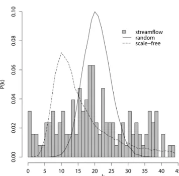
As discussed in the introduction, we can place the stream-flow network in context with the known network topologies by computing three network properties, the degree distribu-tion (P (k)), the clustering coefficient (C), and the average path length (L). We begin by computing the degree distri-bution for the streamflow network and comparing it to the expected distribution for regular, random, and scale-free net-works having the same number of nodes and links (Fig. 4). The streamflow network degree distribution is characterized by a weak peak centred at about 19 degrees (corresponding to the mean), which is flanked by symmetric, broad, and noisy wings. The noise arises from the relatively low number of nodes in the network compared to some other applications, such as the Internet. From Fig. 4, it is immediately clear that the streamflow network is not a regular network because, by definition, each node in a regular network has the same number of links, i.e.,P (k)=δk, whereδk is the Kronecker
delta function located at a single value ofk. Furthermore, the streamflow network degree distribution is not consistent with the expected degree distribution for a scale-free network be-cause scale-free networks have an asymmetric degree distri-bution which asymptotes toP (k)∝k−γ at sufficiently large values ofk, whereγ ranges from 2.1 to 4 for a wide array of observed networks (Barabási and Albert, 1999). The
stream-Figure 3.Georeferenced representation of the streamflow network.
A line is drawn between each pair of stations if their linear corre-lation coefficient exceeds 0.7. The station colours are based on the WSC designated subregion as in Fig. 2.
Figure 4.Discrete representation of the degree distribution for the
flow network degree distribution, on the other hand, bears some resemblance to the degree distribution for a random network, which is a binomial distribution. The random net-work has a narrower peak and lower tails in comparison.
Therefore two possibilities remain – small-world (but not scale-free) or random. The difference between these cases lies in the clustering coefficient and average path length. A network is considered small-world if C≫Crandom and L&Lrandom(Watts and Strogatz, 1998). The streamflow
net-work has a global clustering coefficient ofC=0.69 and an average path length ofL=3.03, whereas the equivalent ran-dom graph has a clustering coefficient of Crandom=0.15,
and a path lengthLrandom=1.88. Therefore the streamflow
network satisfies the conditions for a small-world network. Thus, the streamflow network is an example of a small-world network that does not exhibit scale-free behaviour. This is uncommon but not unprecedented. Examples of small-world networks that do not have power law distributions are dis-cussed in Amaral et al. (2000).
As noted in the introduction, small-world networks are characterized by stability and efficiency. A stable network is one that retains its integrity even if nodes are removed be-cause of the high degree of clustering. In other words, the removal of a node at random will likely not fragment the net-work. In the context of the streamflow network, this means that if a randomly selected station is removed then it should be possible to recover most of its information through the interdependence of the stations. Network efficiency is some-times thought of as the ease with which information prop-agates across the network. A network with a small average path length is highly efficient because two arbitrary nodes are likely to be separated by only a few links.
3.3 Sensitivity tests
While assigning links to stations sharing a correlation coef-ficient in excess of 0.7 assures that the links are statistically and intuitively meaningful, one might question whether the specific threshold value has any impact on the structure of the network. An excessively low threshold, below perhaps 0.4 or so, causes identification of links where, in general, none ex-ists in any statistically or (potentially) physically meaningful way. In the limit ofrt→0, the network becomes fully
con-nected with what are largely spurious links, which is not in-teresting or useful. At the other extreme, an excessively high threshold would lead to identification of links only between extremely closely related stations, leaving many unconnected nodes, which again is not very meaningful. For example, at rt=0.9, 30 % of the nodes in the streamflow network are
completely isolated. Similar behaviour was observed in the network-based analysis of climate by Tsonis and Roebber (2004), who note a large fraction of disconnected nodes when rt=0.9, which serves to distort the network.
However, there is still a range of reasonable threshold val-ues which deserve some attention. To assess whether global
network properties of the streamflow network are sensitive to the choice of threshold, we evaluated the network for two additional values of the selected threshold,rt=0.6 and rt=0.8. This is similar to the range considered by Sivakumar
and Woldemeskel (2014) in their sensitivity analysis, and for similar reasons. We then calculated the degree distribution, clustering coefficient, and average shortest path length for each of these alternative threshold values, and compared the results to what would be expected for several idealized net-work architectures.
The streamflow network degree distribution undergoes a few obvious changes whenrt is varied (Fig. 5). For
exam-ple, both the average and maximum degree decrease with in-creasingrt. However, there is little evidence of a
fundamen-tal change in network topology, as the streamflow network still does not appear to strictly fit the degree distributions expected for regular, random, or scale-free networks as dis-cussed above. Some asymmetry in the streamflow network degree distribution begins to appear atrt=0.8, but as noted
earlier, the network becomes increasingly fragmented and less meaningful at very highrt. The streamflow network
de-gree distribution bears some similarity to a random network degree distribution atrt=0.6; however, as we will show, the
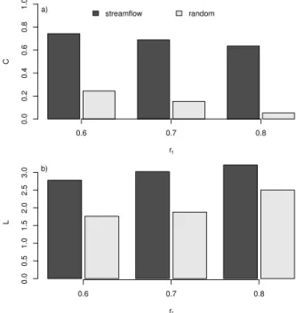
clustering coefficient and average path length indicate that the streamflow network is not a random network. The clus-tering coefficient has only a weak dependence on the thresh-old correlation, decreasing from 0.74 to 0.64 asrtincreases
from 0.6 to 0.8 (Fig. 6a). More importantly, it is always much larger than the expected value for an equivalent idealized ran-dom network. Similarly, the average path length increases from 2.8 to 3.2 over the range of 0.6≤rt≤0.8 (Fig. 6b),
but it remains only slightly higher than what would be ex-pected for the equivalent random network. In summary, then, our inference that these streamflow data are consistent with a small-world network topology appears insensitive to reason-able perturbations of the correlation threshold used for link definition.
A change in global network properties as a function of correlation threshold was observed by Tsonis and Roebber (2004) in their analysis of climate. They argue, however, that there is no fundamental change in the network structure be-cause the clustering coefficient always remains higher than what would be expected for a random network. The same conclusion can be drawn for the streamflow network because the clustering coefficient and average path lengths satisfy the criteria for small-world networks for reasonable values ofrt,
as discussed above. The implication, then, is that the choice may not be critically important to overall network character-ization.
Figure 5.Degree distribution,P (k), for three values of the correla-tion coefficient threshold,rt, for the streamflow network (grey bars).
Also shown are the ensemble means of the expected degree distri-butions for a random network (solid line) and a scale-free network withP (k)∝k−2for largek(dashed line). The random and scale-free networks were configured to have the same number of vertices and edges as the streamflow network.
0.6 0.7 0.8
streamflow random
rt
C
0.0
0.2
0.4
0.6
0.8
1.0 a)
0.6 0.7 0.8
rt
L
0.0
0.5
1.0
1.5
2.0
2.5
3.0 b)
Figure 6.Network clustering coefficient,C, and average shortest
path length,L, for the streamflow network and the equivalent ran-dom networks for three values of the correlation coefficient thresh-old,rt.
from the data because much of the variance in streamflow is associated with seasonality. Use of Spearman correlation has a tendency to increase the number of links between sta-tions because rank correlation allows for more complex (yet monotonic) relationships. However, these choices do not af-fect the global network structure as diagnosed by the cluster-ing coefficient or average path length. Note also that when making the decision to use absolute or anomalous values, we may additionally refer back to one of the major impe-tuses for this paper, which is to use network theory to as-sess how well the current array of streamflow gauges sam-ples the hydrology of the Coast Mountains and to explore how network theoretic insights might help guide future deci-sions on streamflow monitoring system design. That is, the emphasis lies on actual river flows, as might be required for water supply, ecology, civil engineering, or other potential applications. These actual discharge values are influenced to a considerable degree by seasonal forcing, and therefore re-quire direct sampling by a hydrometric monitoring system. Additionally, sharing a common seasonal flow regime, espe-cially within our study region (where seasonal regimes ex-hibit great basin-to-basin heterogeneity as discussed in detail above), is a fundamentally meaningful and operationally im-portant physical link between two stations. That is, we would in general wish the network analysis, and a streamflow mon-itoring system, to directly capture such connections. Further discussion on the use of anomalous values of geophysical data and network analysis can be found in Tsonis and Roeb-ber (2004).
4 Community structure
Many networks consist of distinct groups of highly intercon-nected nodes, which are often referred to as communities. This is particularly true of small-world networks observed in nature (Girvan and Newman, 2002), and also of the stream-flow network, as we will show.
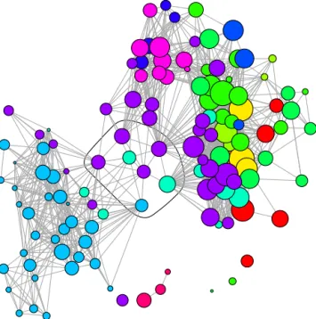
Consider Fig. 7, an alternative representation of the streamflow network in which the stream gauge station po-sitions are not georeferenced. Instead, the nodes were ar-ranged by an algorithm which determines the positions in such a way as to clearly present the network structure (Ka-mada and Kawai, 1989). This particular representation sug-gests that there are two dominant groups in the streamflow network: Vancouver Island and everything else.
Figure 7.Graph representation of the streamflow network. The ver-tices were arranged by the algorithm of Kamada and Kawai (1989). The colours represent the WSC designated subregion as in Fig. 2. The stations inside the black circle are a subset of the stations hav-ing a high value of betweenness.
4.1 Algorithms and sensitivity testing
Many algorithms have been developed to find community structures in graphs (see Fortunato, 2010, for an extensive review). The number of algorithms is due to, in part, the fact that there is no strict definition of a community (Fortunato, 2010). Furthermore, the task of community detection is, in general, computationally intensive, and the proliferation of network theoretic algorithms for community detection has been partly driven by the development of fast approximate methods, which are necessary for large networks.
Given the rather imprecise definition of a community, we cannot expect that there will be a single correct algorithm which can find the one true answer. Thus the task of choos-ing an algorithm comes down to practical considerations. For example, run times can vary considerably between the algo-rithms because the computational costs of some scale linearly with the number of nodes or edges, while others scale expo-nentially (Danon et al., 2005). Our own testing even suggests that the underlying network topology can affect the run time for an algorithm even when the number of edges and vertices are held constant.
Although we cannot assess whether an algorithm can find the single true answer (if such a thing exists), we can com-pare the algorithms to see if they find the same answer. We therefore applied eight such algorithms to the hydrologic data: walk trap, fast greedy, leading eigenvector, edge
be-tweenness, multi-level, label propagation, info map, and op-timal. A review of these various algorithms is beyond the scope of our article. Interested readers may refer to For-tunato (2010) for further background, and a description of the algorithm we ultimately selected is provided below. The streamflow network community structure identified by the various algorithms was then compared using the normalized mutual information (NMI) index, a measure of the similarity of clusters (Danon et al., 2005). This index is normalized on the interval of 0–1, and high values indicate that two algo-rithms produce similar community structures. In the case of the streamflow monitoring network, the NMI index varies be-tween 0.81 and 1.00 for the eight different algorithms tested (Table 1). This indicates that the results are not particularly sensitive to the community detection algorithm.
In addition to finding similar community structures, the al-gorithms return a similar, but not identical, number of com-munities (between 8 and 10). In general, all of the algorithms find three large communities, and five to seven smaller ones. The three largest communities contain between 84 and 94 % of the total number of stations. All of the algorithms find a handful of communities which contain only one member (station nos. 08AA009, 08EE025, 08FF006, and 08MH029). This is a trivial result (in a strictly graph theoretic sense) because these particular stations have no links to the net-work. The edge betweenness algorithm (discussed below) also identified a community composed of a single station which, unlike the cases just mentioned, had links to other stations (08AA008, two links).
If we consider the reasonable consistency in the number of communities found by each algorithm, the tendency for most stations to fall within three large communities, and the high NMI scores, it is apparent that choice of algorithm is not of critical importance. We therefore proceed by using the edge betweenness algorithm to isolate the communities because it is well documented, and because its NMI index ranges from 0.86 to 0.94, indicating a good agreement with the other al-gorithms.
The edge betweenness algorithm works as follows. The algorithm identifies communities by finding bottlenecks (or bridges) between highly clustered regions of the graph. These bridges are found by exploiting a property known as edge betweenness (Girvan and Newman, 2002; Newman and Girvan, 2004). Edge betweenness is the number of shortest paths between all combinations of node pairs which pass through a particular edge. It is an extension of the concept of node betweenness, which is itself a useful property that will be used and discussed in Sect. 4.3.
larger-Table 1.Comparison of community detection algorithms with the normalized mutual information (NMI) index (Danon et al., 2005).
Algorithm WT FG LE EB ML LP IM O
WT 1.00 – – – – – – –
FG 0.97 1.00 – – – – – –
LE 0.97 0.95 1.00 – – – – –
EB 0.94 0.91 0.94 1.00 – – – –
ML 0.87 0.89 0.87 0.88 1.00 – – –
LP 0.92 0.91 0.90 0.86 0.83 1.00 – –
IM 0.87 0.90 0.88 0.91 0.86 0.81 1.00 –
O 0.87 0.89 0.87 0.88 1.00 0.83 0.86 1.00
WT: walk trap; FG: fast greedy; LE: leading eigenvector; EB: edge betweenness; ML: multi-level; LP: label propagation; IM: info map; and O: optimal.
scale communities into progressively smaller ones in a den-dritic fashion. At each step, a measure of the optimal commu-nity structure called modularity is calculated (Newman and Girvan, 2004). Roughly speaking, high-modularity networks are densely linked within communities but sparsely linked between communities. In practice, the iteration is terminated when modularity reaches a maximum.
4.2 Community structure in the streamflow network Application of the edge betweenness algorithm to the stream-flow network sorts the stations into 10 communities. Com-munities 3, 4, and 8 are the largest, and together they contain 90 % of the stations. Five communities consist of a single sta-tion. A summary of the community membership, along with a basic description of a typical station in each community is given in Table 2, while a table of the complete community membership is given in Table A1.
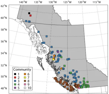
The geographic distribution of the communities is mapped in Fig. 8. The most striking result is that the spatial extent of the communities is variable; some communities are lo-calized, while others are dispersed widely over the domain. For example, community 3 consists of mainland stations lo-cated throughout the Coast Mountains, while community 4 consists primarily of stations in the southeasternmost Coast Mountains except for a few stations further north. Commu-nity 8 consists entirely of stations on the southwesternmost British Columbia mainland and on Vancouver Island. Most communities do not map in a straightforward way onto the geographic regions defined by the WSC station designation prefix (Fig. 2).
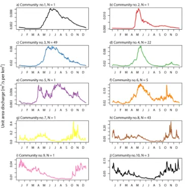
If the streamflow communities are not solely defined by the geographic distribution of their members, then what forms them? The answer must lie in the hydrographs, since the network was defined by their covariance. To investi-gate this, a representative hydrograph was computed for each community by first forming a median annual hydroclimatol-ogy for each station using the same 10-year time series that defined the network. The climatological median discharge for each station was then normalized by drainage area to form the unit area discharge. Finally, the median unit area
hydro-Table 2.Summary of the community analysis. The communities
were found using the edge betweenness algorithm (Girvan and Newman, 2002; Newman and Girvan, 2004).
Community Number of Geographic description number members
1 1 (<1 %) Yukon, high elevationa
2 1 (<1 %) Yukon, high elevation
3 49 (39 %) Wide geographic range, high elevation 4 22 (17 %) Southern BC, mid-elevationb
5 1 (<1 %) Central BC, mid-elevation, small drainage 6 5 (4 %) Central BC, mid-elevation
7 1 (<1 %) Central BC, low elevationc, small drainage 8 43 (34 %) Southwestern BC and Vancouver Island,
low elevation
9 1 (<1 %) Southwestern BC, near sea level 10 3 (2 %) Haida Gwaii, low elevation a>1200 m,b≈1000 m,c<800 m.
Figure 8.Streamflow station map coloured according to
commu-nity membership. The communities were identified with the edge betweenness algorithm (Girvan and Newman, 2002; Newman and Girvan, 2004).
graphs were averaged by community to form a representative annual hydrograph.
hy-Figure 9. Representative unit area hydrographs for each of the 10 communities. The hydrographs were created by averaging the 10-year median climatology for all stations within the community. The line colours are consistent with the map in Fig. 8, except for the community 10, which is plotted here in black.Ngives the number of hydrometric stations within each community.
drologic regime typing. Conversely, all four of the canonical hydrographs are represented by at least one community.
How can two stations of the same hydrologic type be poorly correlated? The average annual cycle and its overall physical controls are only one aspect of a river’s dynamical properties. As an example, consider two small pluvial basins, one on an island of Haida Gwaii on the northern BC coast, and the other 800 km away on Vancouver Island on the south-ern BC coast. Although peak flow for both stations occurs in winter, when rainfall is highest, the rainfall is episodic because it is caused by frontal systems embedded in low pressure cyclones. Even if the same weather system impacts both stations, the travel time between stations will create a phase lag which is large enough compared to the falling limb to create a weak zero-lag correlation. More importantly, in many cases a specific storm will affect one region but not an-other 800 km away. Indeed, precipitation teleconnections to El Niño–Southern Oscillation and the Pacific Decadal Oscil-lation differ fundamentally between the southern and north-ern BC coasts (Fleming and Whitfield, 2010). It seems clear that such disconnected meteorological forcing is why com-munities 8 and 10 are distinct in spite of having very similar median annual hydrographs.
A similar argument can be made for nival stations, al-though the mechanisms might be different. Day-to-day, basin-to-basin variability in the snowpack and/or melt rates
(set by temperature or rain-on-snow events) can affect peak flow timing or the length of the falling limb, and therefore impact the correlation between two stations. Although the dominant forcing causing snowmelt is seasonal, the spatial scale of specific forcing anomalies (i.e., weather) could eas-ily create spatial variability on scales smaller than the dis-tance separating two different nival basins.
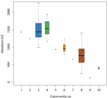
It is also interesting to explore how these network the-oretic communities might reflect different catchment prop-erties. For example, both the day-to-day streamflow dy-namics and the overall seasonal hydrologic regime exhib-ited by data from a particular hydrometric station are de-termined to a significant extent by the elevation of the up-stream basin area since in the Coast Mountains elevation de-termines in large part whether the basin receives daily pre-cipitation as rain, snow, or some mixture of the two, and also what time of year the corresponding runoff occurs. Thus it might be possible to understand the community struc-ture, at least in part, in terms of basin elevation. Consider Fig. 10, which summarizes the distribution of mean drainage elevations for the stations within each community. The fig-ure shows that the communities are, to some degree, strat-ified by elevation. Communities 1 through 4 represent sta-tions which sample high-elevation basins (loosely defined here as>1200 m), communities 5 and 6 represent middle-elevation stations (≈1000 m), while 7 through 10 represent low-elevation stations (<800 m). Cross referencing this with the map in Fig. 8, we see that community 3 contains the high elevation stations which span most of the Coast Mountains, community 4 mostly contains the high elevation stations in the southeastern Coast Mountains, and community 8 con-tains low-elevation stations from southwestern BC and Van-couver Island.
Figure 10.Boxplots of mean basin elevation grouped by commu-nity. The colours are consistent with the map in Fig. 8.
Figure 11. Boxplots of upstream basin drainage area grouped by
community. The colours are consistent with the map in Fig. 8.
Alternatively, the division between communities 3 and 4 might also be driven by the increased likelihood for stations in community 3, which extends further north than commu-nity 4, of having more permanent ice coverage or a thicker snowpack. Unfortunately this cannot be tested quantitatively because ice cover data were not readily available for about half of the stations in this analysis. However, mid-to-late summer differences in median hydrograph form are consis-tent with this interpretation, with community 3 exhibiting a more seasonally extensive melt freshet than community 4 (Fig. 9).
4.3 Additional network metrics – betweenness
The edge betweenness community detection algorithm placed 90 % of the stations into three communities, while the remaining 10 % fell within single-member and small-membership communities. Small-small-membership communities have daily streamflow dynamics that are uncommon because they represent undersampled and/or rare hydrometeorologi-cal regimes, which we will argue makes them important if the goal of a hydrometric network is to sample the inherent hy-drometeorological diversity of the Coast Mountains. As we will show here, there are also several additional important stations which were not directly identified by the community analysis.
A closer inspection of the streamflow network representa-tion in Fig. 7 reveals a handful of starepresenta-tions which are posi-tioned in-between the large communities. These stations be-long to large communities, but unlike most stations they tend to possess intercommunity connections. Such stations act as bridges between communities, and thus they can be regarded as hybrid stations representing the transition between station groups having different day-to-day hydrometeorological dy-namics and even annual regime types.
The local network property that sets them apart is called betweenness, a concept we broached briefly in our discus-sion of community detection algorithms. Formally, the be-tweenness of a node is the number of geodesic paths passing through it, where a geodesic path is the shortest path between a node pair. In fact, the concept of edge betweenness, which was used to identify the community structure, is an exten-sion of the concept of node betweenness. A high between-ness node would host a great amount of geodesics in the same way that a bridge hosts a great amount of traffic in a trans-portation network. As for the community-finding process, no assumptions are required regarding network topology.
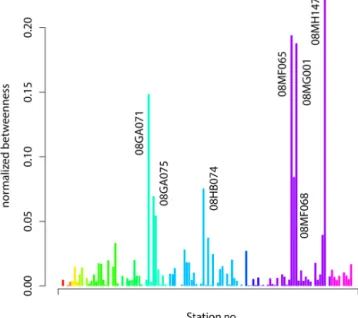
The bar plot in Fig. 12 shows that node betweenness is un-evenly distributed across the streamflow stations such that a small number of stations have very high scores, while most stations have low scores. The high scores are of interest here, so for the purpose of discussion we select stations having a (somewhat arbitrarily chosen) normalized betweenness score of 0.06 or higher. There are seven stations fitting this crite-rion: 08GA071, 08GA075, 08HB074, 08MF065, 08MF068, 08MG001, and 08MH147. These seven stations are encircled in Fig. 7.
clima-Figure 12.Bar plot of the betweenness scores for every station, with several high-betweenness stations highlighted. The station colours are based on the WSC designated subregion shown in Fig. 2.
tological hydrographs for each of these seven stations resem-bles the mixed rain–snow regime (e.g., Fig. 1c).
In terms of network theory, high-betweenness stations are important to network stability given their role as bridges be-tween communities. For this reason we argue that they are essential members of the network, but not in the same way as the stations forming the small-membership communities. The loss of just a few high-betweenness stations would frag-ment the network into isolated communities. Information flow, or in our context, transferability of discharge measure-ments across locations, would be restricted in their absence.
5 Implications for the streamflow monitoring network The various network diagnostics and tools have provided micro-level (i.e., individual stations) and macro-level (com-munity structure and network architecture) descriptions of the streamflow network. The question now becomes: how can we use these results to inform and guide streamflow work design? We begin by first summarizing what the net-work analysis told us about the data from the current mon-itoring system. As discussed above, the architecture of the streamflow network is consistent with the small-world class of networks. Small-world networks are considered stable, meaning that the removal of a node at random is unlikely to fragment the network. In terms of the streamflow monitor-ing system, this implies there may be a sufficient amount of redundant information, or a relatively large number of station pairs with high correlation coefficients. A randomly selected station will likely have 19.6 connections (the network-wide node degree average). As such, the loss of any one station
selected at random will probably not result in the loss of a significant amount of information or a fragmented network. However, if a high-betweenness station is lost, then the like-lihood of fragmenting the network is increased. Moreover, the loss of a station which belongs to a single-membership community is essentially the loss of unique and therefore un-recoverable information because there is no means to recon-struct its streamflow.
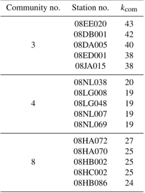
The edge betweenness community detection algorithm identified 10 communities within the streamflow network, but 90 % of the stations fell within just 3 communities. A community, defined on the basis of network theoretic analy-sis, shares specific elements which can be tied back to two general physical hydrologic characteristics: mean annual hy-drograph form reflecting similar precipitation phasing in this transitional rain–snow region, in turn largely a function of basin elevation or secondarily latitude and continentality, and geographic proximity reflecting shared day-to-day local-to-synoptic scale meteorological forcing. Therefore, the num-ber of communities reflects the hydrometeorological diver-sity of the Coast Mountains, and the number of stations per community sets the extent to which each distinct hydrologic “family” is sampled. The stations within each community having the highest number of intracommunity links can be thought of as index or reference stations (explicitly summa-rized for the three largest communities in Table 3; select-ing an index station is obviously less necessary or useful for smaller communities). Such stations have streamflow time series that are representative of the other members of their re-spective communities. Because the distribution of intracom-munity degrees was somewhat evenly distributed across the stations, no single station can clearly be identified as the sole index for each of the large communities, and presumably any of those short-listed in Table 3 would suffice for its respective community.
The community-detection and node-betweenness algo-rithms identified two types of “outlier” stations. The first type consists of those stations belonging to small-membership communities. These stations represent rare or undersampled hydrometeorological regimes. Such communities may ex-hibit a median annual hydrograph similar to other commu-nities, but they appear to be sufficiently distant in space that they do not, in general, share the same meteorological forc-ing with those other communities. Thus, the streamflow time series from one such community cannot be accurately in-dexed by, or easily reconstructed from, the streamflow time series from another.
Table 3.The most highly connected (in an intracommunity sense) stations in each of the three largest communities and the number of intracommunity links (kcom). These stations could serve as index
stations for their respective community.
Community no. Station no. kcom
08EE020 43 08DB001 42 3 08DA005 40 08ED001 38 08JA015 38
08NL038 20 08LG008 19 4 08LG048 19 08NL007 19 08NL069 19
08HA072 27 08HA070 25 8 08HB002 25 08HC002 25 08HB086 24
network, in principle making it more difficult to recover in-formation.
There is a substantial amount of redundancy (many pairs of stations with a high correlation coefficient) within the three large communities identified in this paper. Stations hav-ing a low betweenness score, a high number of degrees, and membership to a large community might be regarded as re-dundant and thus, perhaps, candidates for decommissioning under, for example, budgetary pressure. However, the net-work theoretic perspective suggests that this type of redun-dancy could alternatively be considered a strength of the hy-drometric monitoring system, insofar as it implies that the stream gauges, in their present arrangement, form a stable network which is resilient to the unintended loss of a node (as might occur operationally due to equipment failure, for example). Much of the high interconnectedness within each of the three large communities may simply be driven by sea-sonal snow and ice melt from mid- to high-elevation basins, or, in the case of the pluvial drainages of Vancouver Island and the low-elevation regions of southwestern BC, a dense array of gauges sampling a sufficiently small region.
Given the insights gained by analyzing the current net-work, what might the optimal sampling network look like? As discussed in the introduction, this depends on many practical considerations which are far beyond the scope of this study and, perhaps, any statistical data analysis-based method for hydrometric monitoring system design. Some of these considerations include budget constraints, station ac-cessibility, or special applications (such as fisheries stud-ies, climate variability and change detection, or the need to monitor a particular river for a particular purpose, such as
an assessment for microhydropower generation potential or the design of bridge crossings, for example). In the absence of these considerations, or in addition to them, a sampling program would ideally capture all of the possible types of streamflow dynamics in the region. In the context of network theory, this amounts to maximizing the number of commu-nities sampled because the number of commucommu-nities reflects hydrometeorological diversity. The number of members in each community should be large enough to provide some re-dundancy as a safeguard to ensure minimal information is lost if a station fails or is decommissioned; that said, redun-dancy might also be viewed as an argument in favour of sta-tion closure, as noted above. In any event, the small number of stations having high betweenness, and the stations which are members of a small community, constitute two types of particularly high-value stations which should not be removed from the streamflow monitoring system under cost-cutting, for example. Additionally, stations with a high number of intracommunity links might be identified as index or refer-ence stations for their respective communities, and should be viewed as high-value stations.
6 Conclusions
In this paper, we have analyzed the hydrology of the Coast Mountains by applying network analysis tools to a collection of streamflow gauges. Our motivation was to characterize the existing network and place it in context with idealized and observed networks, with an eye to informing streamflow net-work design.
Daily streamflow data in this region proved amenable to network theoretic analysis. In particular, it was found to display properties consistent with the small-world class of networks, a common type observed in many disciplines. A small-world network implies stability, and that its structure is resilient to the loss of nodes. Interestingly, the results also suggest that the streamflow network in this region is not of the scale-free type. There is precedent for small-world, non-scale-free networks, but they appear uncommon.
The network theoretic outcomes provide a different way of viewing spatiotemporal hydrologic patterns and, in partic-ular, a novel perspective on the old question of optimal hy-drometric monitoring system design. We argue that the ideal-ized sampling strategy should span the full range of dynam-ical classes described above, and additionally that it should retain some redundancy in the event of station failure, which may be facilitated by the small-world topology identified for this network. Furthermore, we identified a number of sta-tions which warrant special attention because they character-ize rare, undersampled, or information-rich hydrometeoro-logical dynamics. Specifically, we propose that from a mon-itoring system design perspective, the most important sta-tions are (1) those which have a large number of intracom-munity links and thus serve as indices for their respective communities, (2) those with high betweenness values, and which thus serve as do-it-all stations embedding information about multiple communities, and (3) those which are mem-bers of single-memmem-bership or small-memmem-bership communi-ties, as their hydrometeorological dynamics are poorly sam-pled by the existing monitoring system and cannot be readily reconstructed from other hydrometric stations.
The network analysis as applied in this paper required us to choose a number of parameters. For example, it was nec-essary to fix the threshold correlation coefficient to define the pairwise relationships between streamflow gauges. We reit-erate that our analysis showed that the network architecture, a global property, is not sensitive to the threshold coefficient within a realistic range of values. However, we do expect that changing the coefficient will likely impact the details of com-munity membership and the individual high-value stations identified by community detection and betweenness. This is obviously due to the fact that some pairwise relationships will simply change as the threshold correlation coefficient is varied. Care should be taken to understand which stations share correlation coefficients near the threshold before using a community or betweenness analysis to guide practical deci-sions on whether to alter the streamflow monitoring system.
In addition to hydrometric monitoring system design, this work will hopefully inspire further applications of network theory to regional hydrology. As such, and given the relative newness of network theoretic applications within water re-sources science as discussed in the introduction, one could envision any number of (potentially) useful extensions or re-finements. A few are listed as follows. Repeating the analysis with deseasonalized discharge time series might be interest-ing because it would remove the seasonally driven compo-nent of serial correlation, and therefore more clearly reveal regional climate or weather effects, but might be less useful for hydrometric network design as it would not speak directly to actual streamflow values. The analysis could also be re-peated with time periods of different lengths, or with climate-conditioned networks formed by selecting data from partic-ular seasons or years (e.g., winter only, or El Niño years). Application of the methods in different regions could prove
Appendix A: Streamflow community membership The edge betweenness community finding algorithm identi-fied 10 communities within the streamflow network. In Ta-ble A1 we provide a complete list of the members in each community.
Table A1.Membership table of the communities in the streamflow network as determined by the edge betweenness algorithm.
Community Water Survey of Canada station number
1 08AA008
2 08AA009
08AB001 08AC001 08AC002 08BB005 08CE001 08CF003 08CG001 08DA005 08DB001 08DB013 08DB014 08EB004 08EC013 08ED001 08ED002 08EE004 08EE008 08EE012 08EE020 08EF001 08EF005 3 08EG012 08FA002 08FB006 08FB007 08FE003 08GA071 08GA072 08GD004 08GD008 08GE002 08GE003 08JA015 08JB002 08JB003 08MA001 08MA002 08MA003 08MB005 08MB006 08MB007 08ME023 08ME025 08ME027 08ME028 08MF065 08MG005 08MG013 08MG026
4
08EE013 08FC003 08LG008 08LG016 08LG048 08LG056 08MA006 08MF062 08MF068 08MH001 08MH016 08MH056 08MH103 08NL004 08NL007 08NL024 08NL038 08NL050 08NL069 08NL070 08NL071 08NL076
5 08EE025
6 08EG017 08FB004 08FF001 08FF002 08FF003
7 08FF006
08GA061 08GA075 08GA077 08GA079 08HA001 08HA003 08HA010 08HA016 08HA068 08HA069 08HA070 08HA072 08HB002 08HB014 08HB024 08HB025 08HB032 08HB048 08HB074 08HB075 08HB086 8 08HB089 08HC002 08HC006 08HD011 08HD015 08HE006 08HE007 08HE008 08HE009 08HE010 08HF004 08HF005 08HF006 08HF012 08HF013 08MG001 08MH006 08MH076 08MH141 08MH147 08MH155 08MH166
9 08MH029
Acknowledgements. The authors would like to thank Judy Kwan at Environment Canada for her GIS expertise in drainage elevation statistics, and the referees Mishra Ashok and Bellie Sivakumar for their valuable comments.
Edited by: J. Vrugt
References
Abe, S. and Suzuki, N.: Small-world structure of earthquake network, Physica A, 337, 357–362, doi:10.1016/j.physa.2004.01.059, 2004.
Amaral, L. A. N., Scala, A., Barthélémy, M., and Stanley, H. E.: Classes of small-world networks, P. Natl. Acad. Sci. USA, 97, 11149–11152, doi:10.1073/pnas.200327197, 2000.
Archfield, S. A. and Kiang, J. E.: Response of the United States streamgauge network to high- and low-flow periods, abstract H41M-08 presented at the American Geophysical Union Fall Meeting, San Francisco, California, USA, available at: http://abstractsearch.agu.org/meetings/2011/FM/sections/H/ sessions/H41M/abstracts/H41M-08.html, last access: 12 Decem-ber 2014, 2011.
Barabási, A.-L. and Albert, R.: Emergence of scal-ing in random networks, Science, 286, 509–512, doi:10.1126/science.286.5439.509, 1999.
Bras, R. L. and Rodríguez-Iturbe, I.: Rainfall network design for runoff prediction, Water Resour. Res., 12, 1197–1208, doi:10.1029/WR012i006p01197, 1976.
Burn, D. H. and Goulter, I. C.: An approach to the rationalization of streamflow data collection networks, J. Hydrol., 122, 71–91, doi:10.1016/0022-1694(91)90173-F, 1991.
Caselton, W. F. and Husain, T.: Hydrologic networks: information transmission, J. Water Res. Pl.-ASCE, 106, 503–520, 1980. Csardi, G. and Nepusz, T.: The igraph software package for
com-plex network research, InterJournal, Comcom-plex Systems, 1695, available at: http://igraph.org, last access: 12 December 2014, 2006.
da Fontoura Costa, L., Rodrigues, F. A., Travieso, G., and Boas, P. R. V.: Characterization of complex networks: a survey of measurements, Adv. Phys., 56, 167–242, doi:10.1080/00018730601170527, 2007.
da Fontoura Costa, L., Oliveira, O., Travieso, G., Rodrigues, F., Boas, P. V., Antiqueira, L., Viana, M., and Rocha, L. C.: Analyzing and modeling real-world phenomena with complex networks: a survey of applications, Adv. Phys., 60, 329–412, doi:10.1080/00018732.2011.572452, 2011.
Danon, L., Díaz-Guilera, A., Duch, J., and Arenas, A.: Compar-ing community structure identification, J. Stat. Mech.-Theory E., 2005, P09008, doi:10.1088/1742-5468/2005/09/P09008, 2005. Donges, J. F., Zou, Y., Marwan, N., and Kurths, J.: Complex
net-works in climate dynamics, Eur. Phys. J.-Spec. Top., 174, 157– 179, doi:10.1140/epjst/e2009-01098-2, 2009.
Eaton, B. and Moore, R. D.: Regional hydrology, in: Compendium of Forest Hydrology and Geomorphology in British Columbia, edited by: Pike, R. G., Redding, T. E., Moore, R. D., Winkler, R. D., and Bladon, K. D., vol. 1 of Land Management Hand-book 66, Chap. 4, B. C. Ministry of Forests, 85–110, available at:
www.for.gov.bc.ca/hfd/pubs/Docs/Lmh/Lmh66.htm, last access: 12 December 2014, 2010.
Elsner, J. B., Jagger, T. H., and Fogarty, E. A.: Visibility network of United States hurricanes, Geophys. Res. Lett., 36, L16702, doi:10.1029/2009GL039129, 2009.
Flatman, G. T. and Yfantis, A. A.: Geostatistical strategy for soil sampling: the survey and the census, Environ. Monit. Assess., 4, 335–349, doi:10.1007/BF00394172, 1984.
Fleming, S. W.: An information theoretic perspective on mesoscale seasonal variations in ground-level ozone, Atmos. Environ., 41, 5746–5755, doi:10.1016/j.atmosenv.2007.02.027, 2007. Fleming, S. W. and Clarke, G. K.: Glacial control of
wa-ter resource and related environmental responses to climatic warming: empirical analysis using historical streamflow data from northwestern Canada, Can. Water Resour. J., 28, 69–86, doi:10.4296/cwrj2801069, 2003.
Fleming, S. W. and Whitfield, P. H.: Spatiotemporal mapping of ENSO and PDO surface meteorological signals in British Columbia, Yukon, and southeast Alaska, Atmos. Ocean, 48, 122– 131, doi:10.3137/AO1107.2010, 2010.
Fleming, S. W., Moore, R. D., and Clarke, G. K. C.: Glacier-mediated streamflow teleconnections to the Arctic Oscillation, Int. J. Climatol., 26, 619–636, doi:10.1002/joc.1273, 2006. Fleming, S. W., Whitfield, P. H., Moore, R. D., and Quilty, E. J.:
Regime-dependent streamflow sensitivities to Pacific climate modes cross the Georgia–Puget transboundary ecoregion, Hy-drol. Process., 21, 3264–3287, doi:10.1002/hyp.6544, 2007. Fogarty, E. A., Elsner, J. B., Jagger, T. H., and Tsonis, A. A.:
Network analysis of US hurricanes, in: Hurricanes and Climate Change, edited by: Elsner, J. B. and Jagger, T. H., Springer US, New York, USA, 153–167, doi:10.1007/978-0-387-09410-6_9, 2009.
Fortunato, S.: Community detection in graphs, Phys. Rep., 486, 75– 174, doi:10.1016/j.physrep.2009.11.002, 2010.
Girvan, M. and Newman, M.: Community structure in social and biological networks, P. Natl. Acad. Sci. USA, 99, 7821–7826, doi:10.1073/pnas.122653799, 2002.
Hannaford, J., Holmes, M., Laizé, C., Marsh, T., and Young, A.: Evaluating hydrometric networks for prediction in ungauged basins: a new methodology and its application to England and Wales, Hydrol. Res., 44, 401–418, doi:10.2166/nh.2012.115, 2013.
Kamada, T. and Kawai, S.: An algorithm for drawing gen-eral undirected graphs, Inform. Process. Lett., 31, 7–15, doi:10.1016/0020-0190(89)90102-6, 1989.
Martin, E. A., Paczuski, M., and Davidsen, J.: Interpretation of link fluctuations in climate networks during El Niño periods, EPL, 102, 48003, doi:10.1209/0295-5075/102/48003, 2013.
Mishra, A. and Coulibaly, P.: Hydrometric network evalua-tion for Canadian watersheds, J. Hydrol., 380, 420–437, doi:10.1016/j.jhydrol.2009.11.015, 2010.
Mishra, A. K. and Coulibaly, P.: Developments in hydromet-ric network design: A review, Rev. Geophys., 47, 1–24, doi:10.1029/2007RG000243, 2009.
Morrison, J., Foreman, M. G. G., and Masson, D.: A method for estimating monthly freshwater discharge affect-ing British Columbia coastal waters, Atmos. Ocean, 50, 1–8, doi:10.1080/07055900.2011.637667, 2012.
Neuman, S. P., Xue, L., Ye, M., and Lu, D.: Bayesian analysis of data-worth considering model and parameter uncertainties, Adv. Water Resour., 36, 75–85, doi:10.1016/j.advwatres.2011.02.007, 2012.
Newman, M.: The physics of networks, Phys. Today, 61, 33–38, doi:10.1063/1.3027989, 2008.
Newman, M. E. J. and Girvan, M.: Finding and evaluating community structure in networks, Phys. Rev. E, 69, 026113, doi:10.1103/PhysRevE.69.026113, 2004.
Norberg, T. and Rosén, L.: Calculating the optimal number of con-taminant samples by means of data worth analysis, Environ-metrics, 17, 705–719, doi:10.1002/env.787, 2006.
Phillips, J. D., Schwanghart, W., and Heckmann, T.: Graph theory in the geosciences, Earth-Sci. Rev., 143, 147–160, doi:10.1016/j.earscirev.2015.02.002, 2015.
Pires, J., Sousa, S., Pereira, M., Alvim-Ferraz, M., and Martins, F.: Management of air quality monitoring using principal compo-nent and cluster analysis – Part I: SO2and PM10, Atmos.
Envi-ron., 42, 1249–1260, doi:10.1016/j.atmosenv.2007.10.044, 2008. Putthividhya, A. and Tanaka, K.: Optimal rain gauge net-work design and spatial precipitation mapping based on geostatistical analysis from colocated elevation and hu-midity data, Int. J. Environ. Sci. Develop., 3, 124–129, doi:10.7763/IJESD.2012.V3.201, 2012.
R Core Team: R: a Language and Environment for Statistical Com-puting, R Foundation for Statistical ComCom-puting, Vienna, Austria, available at: http://www.R-project.org/, last access: 12 Decem-ber 2014.
Rinaldo, A., Banavar, J. R., and Maritan, A.: Trees, net-works, and hydrology, Water Resour. Res., 42, W06D07, doi:10.1029/2005WR004108, 2006.
Schnorbus, M., Werner, A., and Bennett, K.: Impacts of climate change in three hydrologic regimes in British Columbia, Canada, Hydrol. Process., 28, 1170–1189, doi:10.1002/hyp.9661, 2014. Sen, P. and Chakrabarti, B. K.: Sociophysics: An Introduction,
Ox-ford University Press, OxOx-ford, 2013.
Sivakumar, B.: Networks: a generic theory for hydrology?, Stoch. Env. Res. Risk A., 29, 761–771, 2015.
Sivakumar, B. and Woldemeskel, F. M.: Complex networks for streamflow dynamics, Hydrol. Earth Syst. Sci., 18, 4565–4578, doi:10.5194/hess-18-4565-2014, 2014.
Sivakumar, B., Singh, V. P., Berndtsson, R., and Khan, S. K.: Catchment Classification Framework in Hydrology: Challenges and Directions, J. Hydrol. Eng., 20, Special Issue: Grand Chal-lenges in Hydrology, A4014002, doi:10.1061/(ASCE)HE.1943-5584.0000837, 2015.
Spence, C. and Phillips, R. W.: Refining understanding of hydro-logical connectivity in a boreal catchment, Hydrol. Process., doi:10.1002/hyp.10270, online first, 2014.
Stahl, K. and Moore, R. D.: Influence of watershed glacier cover-age on summer streamflow in British Columbia, Canada, Water Resour. Res., 42, W06201, doi:10.1029/2006WR005022, 2006. Strogatz, S. H.: Exploring complex networks, Nature, 410, 268–
276, doi:10.1038/35065725, 2001.
Suweis, S., Konar, M., Dalin, C., Hanasaki, N., Rinaldo, A., and Rodriguez-Iturbe, I.: Structure and controls of the global vir-tual water trade network, Geophys. Res. Lett., 38, L10403, doi:10.1029/2011GL046837, 2011.
Tsonis, A. A. and Roebber, P.: The architecture of the climate network, Physica A, 333, 497–504, doi:10.1016/j.physa.2003.10.045, 2004.
Tsonis, A. A. and Swanson, K. L.: Topology and Predictability of El Niño and La Niña Networks, Phys. Rev. Lett., 100, 228502, doi:10.1103/PhysRevLett.100.228502, 2008.
Tsonis, A. A., Swanson, K. L., and Roebber, P. J.: What do networks have to do with climate?, B. Am. Meteorol. Soc., 87, 585–595, doi:10.1175/BAMS-87-5-585, 2006.
Tsonis, A. A., Wang, G., Swanson, K. L., Rodrigues, F. A., and da Fontura Costa, L.: Community structure and dy-namics in climate networks, Clim. Dynam., 37, 933–940, doi:10.1007/s00382-010-0874-3, 2011.
Watts, D. J. and Strogatz, S. H.: Collective dynamics of “small-world” networks, Nature, 393, 440–442, 1998.
Whitfield, P. H. and Spence, C.: Estimates of Canadian Pacific Coast runoff from observed streamflow data, J. Hydrol., 410, 141–149, doi:10.1016/j.jhydrol.2011.05.057, 2011.
Whitfield, P. H., Cannon, A. J., and Reynolds, C. J.: Modelling streamflow in present and future climates: examples from the Georgia Basin, British Columbia, Can. Water Resour. J., 27, 427– 456, doi:10.4296/cwrj2704427, 2002.
Whitfield, P. H., Moore, R. D., Fleming, S. W., and Zawadzki, A.: Pacific decadal oscillation and the hydroclimatology of western Canada – review and prospects, Can. Water Resour. J., 35, 1–28, doi:10.4296/cwrj3501001, 2010.
Yamasaki, K., Gozolchiani, A., and Havlin, S.: Climate Networks around the Globe are Significantly Affected by El Niño, Phys. Rev. Lett., 100, 228501, doi:10.1103/PhysRevLett.100.228501, 2008.