Article
Application of SWAT model for assessing effect on main functions of
watershed ecosystem in Headwater, Thailand
W. Sudjarit1,2, Somnimirt Pukngam3, Nipon Tangtham4
1
Graduate School, Kasetsart University, 50 Phaholyothin rd., Chatuchak, Bangkok 10900, Thailand
2
Center for Advanced Studies in Tropical Natural Resources, Kasetsart University, 50 Phaholyothin rd., Chatuchak, Bangkok 10900, Thailand
3
Department of Conservation, Kasetsart University, 50 Phaholyothin rd., Chatuchak, Bangkok 10900, Thailand
4
Forestry Research Center, Kasetsart University, 50 Phaholyothin rd., Chatuchak, Bangkok 10900, Thailand E-mail: [email protected]
Received 6 March 2015; Accepted 5 April 2015; Published online 1 June 2015
Abstract
The Soil and Water Assessment Tool (SWAT) is a well prediction accuracy of agricultural watershed ecosystem depends on how well model input spatial parameters describe the characteristics of watershed. The aim of this study was to assess the effects on watershed ecosystem main functions in terms of water and sediment yield. It was calibrated and validated for streamflow in the watershed to evaluate alternative management scenarios and estimate their effects on watershed functions. The goodness of the calibration results was assessed by the coefficient of determination (R2). Results indicated that the average annual rainfall and streamflow estimations were quite satisfactory. On a daily scale R2 was about 0.69 and a monthly scale was 0.97 which can be considered as acceptable. However, using for the case study of an intensive agricultural watershed ecosystem, it was shown that model versions are able to appropriately reproduce the water balance, nutrients balance, carbon balance, and energy balance. Crop yield, total streamflow and total suspended sediment (TSS) losses calibration were performed using field survey information and data during 2008-2012. This study showed that SWAT model was able to apply for simulating and assessing streamflow, sediment, and nutrients successfully and can be used to study the effects of land use practices on water balance, nutrient balance, carbon balance and energy balance in the small scale of sub-watershed ecosystem as well.
Keywords SWAT model; watershed main functions; watershed ecosystem; Headwater.
1 Introduction
1 Introduction
Agricultural expansion and intensification have altered the quantity and quality of global runoff. Human transformation of global water flows has dramatically impacted ecosystems and the services they generate.
Proceedings of the International Academy of Ecology and Environmental Sciences
ISSN 22208860
URL: http://www.iaees.org/publications/journals/piaees/onlineversion.asp RSS: http://www.iaees.org/publications/journals/piaees/rss.xml
Email: [email protected] EditorinChief: WenJun Zhang
IAEES www.iaees.org Through water withdrawals, land use and land cover changes, agriculture, which covers almost 40% of the terrestrial surface is arguably the major way in which humans change water quantity and quality (Foley, 2005). Agricultural production, and its related hydrological changes, has greatly increased during the 20th century. These changes are expected to continue in the 21st century. Population growth, the production of biofuels and increased meat consumption are driving increased agricultural demands. Nutrient runoff from agricultural fertilizer use has decreased water quality in aquatic ecosystems around the world (Galloway, 2004).
Soil erosion is a major concern for the sustainability of agricultural systems and a threat to the integrity of aquatic ecosystems. Soil erosion can lead to reduction of soil fertility, loss of nutrients, and declines of crop yields in farmlands. In a review of mechanized agricultural systems in which wheat, corn, soybean, and barley were planted, Bakker et al. (2005) found that on average, soil erosion reduced crop productivity by about 4% for each 10 cm of soil lost. The intensity of agricultural activities largely determines the magnitude of soil and nutrient (N, P and K) loss to surface water. As a consequence, sediment yields and leaching of pollutants into surface water can lead to degradation of important aquatic habitat, affect recreational uses of water, and introduce toxins into the human food chain (Gitau et al., 2005). These changes have driven rapid declines in nonagricultural ecosystem services, such as fisheries, flood regulation and downstream recreational opportunities. Despite these impacts, increases in agricultural production have reduced malnutrition and hunger, and agriculture has been an engine of economic growth in many countries.
An improved, synthetic understanding of how such regime shifts are produced is particularly urgent now because of growing demand for water, agricultural products, and other ecosystem services such as carbon sequestration, climate moderation, and erosion control. Climate change that is expected to generate unprecedented alterations in precipitation, soil moisture and runoff will make negotiating the complex hydrology-related ecological trade-offs of agriculture even more challenging. The application of watershed simulation models is indispensable when pollution is generated by a nonpoint source. These models should be able to simulate large complex watersheds with varying soils, land use and management conditions over long periods of time. A wide range of watershed models are available to predict the impact of land management practices on water, sediment and agricultural chemical yields. Examples of these models are the physically based event model ANSWERS (Beasley, 1991), the empirically based SWATCATCH model (Holman et al., 2001), the physically based DWSM model (Borah and Bera, 2003) and the semi-empirical SWAT model (Arnold et al., 1998; Arnold and Fohrer, 2005; Gassman et al., 2007). One common characteristic between all these models is the reproduction of the water and nutrients movement at the watershed scale. Of all the models mentioned previously, the Soil and WaterAssessment Tool (SWAT) is the most capable model for long-term simulations in watersheds dominated by agricultural land uses. This model is designed to assess the impact of land use and management practices on water, sediments and agricultural chemicals in the irrigation returns flows.
a wide range of scales and environmental conditions (Gassman et al., 2007). The objective of this study was to describe the calibration of the SWAT model for flow in the Huai Ma Nai sub-watershed (HMN-SW) by
comparing daily and monthly predicted. The model was then used to assess the effect of land use practices on watershed ecosystem main functions in terms of soil loss, water yield, and sediment yield.
2 Study area and Methodology
2.1 Study site
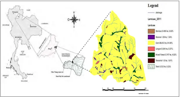
The HMN-SW belongs to the Mae Thang Irrigation area located in the Phrae province in Thailand shown in Fig. 1. The total sub-watershed area is about 96 hectare with elevations ranging from 410 to 465 m above mean sea level.
Fig. 1 Huai Ma Nai sub-watershed localization.
The climate associated with the watershed is in a tropical forest with approximately 106 days per year of rainfall. Annual rainfall, humidity, and daily temperature averages from 1986 to 2011 are 1,177 mm, 86.20%, and 18.10°C, respectively. The rainy season is normally between May to October and dry season between
November to April. Most of the HMN-SW is classified as rolling hill and mountainous area with slope ranging from 12-50%. Soil texture is medium to fine texture with low to medium natural soil fertility, high to medium
natural organic matter content. According to Thai classification system, there are 4 soil series including; Li, MuakLek, Tha Yang, and Wang Saphung. Most of the land (90%) is unsuited for upland crops, only 10% of the area is poorly suited.
2.2 Soil and Water Assessment Tool (SWAT) description
SWAT is a continuous time model that operates on a daily time step, spatially semi-distributed, physically
based model (Arnold et al., 1998). The watershed is divided into multiple sub-watersheds, which are then
IAEES www.iaees.org
sub-basin. The water balance of each HRU is represented by three storage volumes: soil profile (0–2 m), shallow aquifer (typically 2–20 m), and deep aquifer (>20 m). Flow generation, sediment yield, and chemical
loadings from each HRU in a sub-watershed are summed, and the resulting loads are routed through channels, ponds, and/or reservoirs to the watershed outlet. The soil profile is subdivided into multiple layers that consider several soil water processes including infiltration, evaporation, plant uptake, lateral flow, and
percolation. The soil percolation component of SWAT uses a storage routing technique to simulate flow through each soil layer in the root zone. Crop evapotranspiration is simulated as a linear function of potential
evapotranspiration, leaf area index and root depth.
The computations in the SWAT model is based on the premise that the simulation of the hydrology of a watershed can be separated into two major divisions. The first division is the land phase of the hydrologic
cycle. The land phase of the hydrologic cycle controls the amount of water, sediment, nutrient and pesticide loadings to the main channel in each sub basin. The second division is the water or routing phase of the
hydrologic cycle, which can be defined as the movement of water, sediments, etc. through the channel network of the watershed to the outlet. The land phase of the hydrologic cycle is modeled in the SWAT based on the water balance equation:
, , , , ,
where SWt is the final soil water content (mm), SW0 is the initial soil water content (mm), t is the time (days),
Rday,i is the amount of precipitation on day i (mm), Qsurf,i is the amount of surface runoff on day i (mm), Ea,i is
the amount of evapotranspiration on day i (mm), wseep,i is the amount of percolation and bypass flow exiting
the soil profile bottom on day i (mm), and Qgw,iis the amount of return flow on day i (mm).
The sub-basin/sub-watershed components of SWAT can be placed into eight major components including; hydrology, weather, erosion/sedimentation, soil temperature, plant growth, nutrients, pesticides, and land
management. Erosion and sediment yield are estimated for each HRU with the Modified Universal Soil Loss Equation (MUSLE) (Williams et al., 1984). SWAT has been extensively validated across the U.S. for
streamflow and sediment yields (Arnold et al., 1999). Limited validation of the SWAT nutrient simulation has
been attempted. However, in this study, the surface runoff from daily rainfall was estimated using the modified SCS curve number (USDA-SCS, 1972) and the potential evapotranspiration (PET) was determined using the
modified Penman–Monteith approach. The default values provided by the SWAT crop database were used for the crop phosphorus uptake and the optimal plant concentrations (Arnold et al., 1998).
2.3 SWAT input data preparation
ArcSWAT extension of ArcGIS 10.1 was employed in this study. An ArcMap project file that contains links to user retrieved data and incorporates all customized GIS functions into user ArcMap project file. The project
file contains a customized ArcMap Graphical User Interface (GUI) including menus, buttons, and tools. The basic input data included the digital elevation model (DEM), land use map, soil map, and climate data for the
HMN-SW. Three basic files needed by ArcSWAT were for delineating the basin into sub-basins and HRUs including; (1) the DEM was interpolated from topo to raster, (2) soil data were obtained from soil survey map provided by Land Development Department (LDD), and (3) the land use types. The summary of crop and land
Table 1 Summary of crop and land use types in the Huai Ma Nai sub-watershed.
Land use SWAT code Area
Area (ha) % of watershed
Maize CSIL 82.63 96.47
Deciduous forest FRSD 1.95 2.28
Orchard ORCD 1.07 1.25
Soil Soil-62 81.88 95.60
Soil-47 3.77 4.40
Slope
0-5 0.83 0.97
5-25 58.09 67.82
25-9999 26.73 0.97
The major crops are maize and soybean. Every season the farmers were planted soybean after they were harvested the maize in the same area, which cover 96.47% of the entire watershed area. Deciduous forest areas
account for 2.28% of the total watershed area. In this sub-watershed, there are two soil groups namely soil-62 (95.60%), and soil-47 (4.40%). Regarding to climate data, SWAT requires daily precipitation, maximum and
minimum air temperature, solar radiation, wind speed, and relative humidity.
The ArcSWAT2012 was used to delineate the boundaries of the entire study area and its sub-basins, along with their drainage channels. The HMN-SW was divided into 29 sub-basins corresponding to 29 existing
discharge and water quality monitoring stations. The total area of the HMN-SW determined by ArcSWAT was 85.65 hectare, which is smaller than the actual site study because there were some discrepancies between the
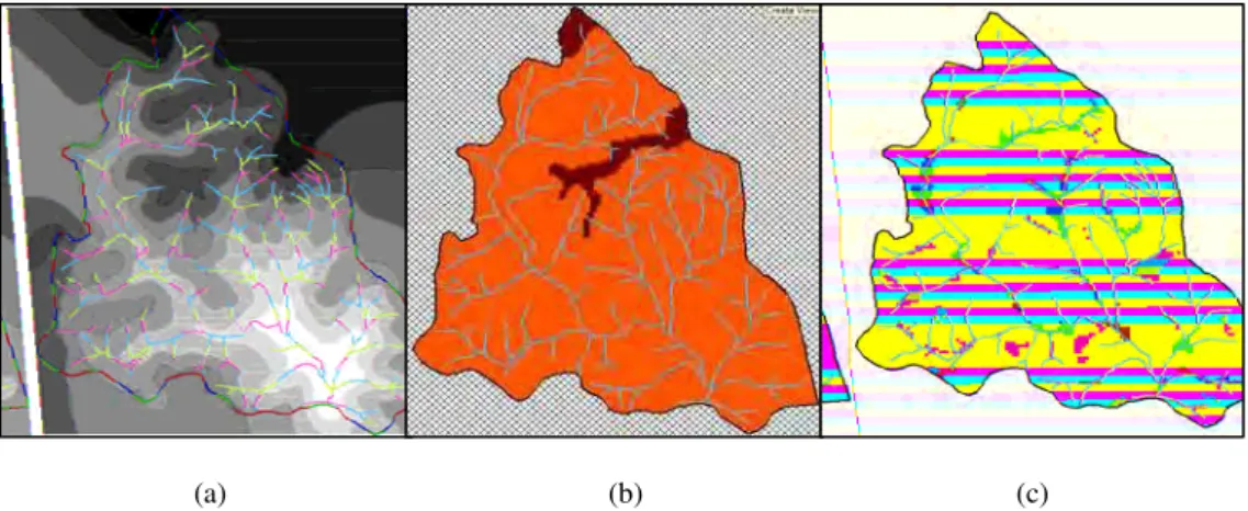
boundary definition by SWAT and the boundary surveyed in the field. Physical characteristics of each of sub-basin and channel attributes are shown in Fig. 2 and Fig. 3. With SWAT threshold levels of 10% was used to land use and soil map. Total of 81 HRUs were defined by ArcSWAT in the HMN-SW.
Fig. 2 Spatial data for SWAT model input (a) DEM (b) a soil group map and (c) a land use map of theHuai Ma Nai sub-watershed.
IAEES www.iaees.org
Fig. 3 Total of 29 sub-basins and 81 HRUs in the Huai Ma Nai sub-watershed.
The unique source of irrigation is from outside the watershed. The weather input data, including maximum and minimum daily air temperature, solar radiation, wind speed and relative humidity were obtained
from the HMN-SW meteorological station, located at North latitude of 18°14ʹ, and East longitude of 100°24ʹ
with altitude of 421 m above mean sea level. Parameters of farmers’ current management operations such as tillage, planting dates, fertilization, irrigation and harvesting were provided as inputs to the model. The
amounts of organic and inorganic fertilizers applied to each crop grown in the MHN-SW were determined through farmer’s interviews and collected soil carbon sequestration in planted and soil with maize and soybean
performed during the 2010 and 2011 planted seasons. 2.4 SWAT calibration and assessment application
SWAT input parameters are physically based and are allowed to vary within a realistic uncertainty range for
calibration (Gassman et al., 2007). Simulations were carried out from January 1st, 2008 to December 31st, 2012
using the standard split sample calibration–validation procedure (Klemeš, 1986). The period from January 1st,
2008 to December 31st, 2008 served as the warm up period for the model in order to take for granted realistic
initial values for the calibration period. Data from January 1st, 2009 to December 31st, 2009 were used for the
calibration and the remaining data for validation. For SWAT simulation, the summary input file (input.std), the
summary output file (output.std), the HRU output file (output.hru), the sub-basin output file (output.sub), and the main channel or reach output file (output.rch) were generated. The output.rch file contains the summary for
each routing each in the watershed and its data were used for the calibration and validation processes. For the hydrological model calibration and validation, the observed streamflow values were compared with the
FLOW_OUT values. The simulated sediments yields (SED_OUT) were compared with the total suspended sediments measured at the outlet.
2.5 Simulation and assessment of watershed main functions on water and sediment yields
After the basic climate and hydrological parameters were calibrated, SWAT was applied to simulate the impacts of main functions (water balance, nutrient balance, carbon balance, and energy balance) on water and
sediment yields for the period of 2008–2012. First, the calibrated SWAT model was run using the input data set of 2008–2012 without modification of any parameters. Results from this run served as the baseline scenario. Second, the water balance, surface runoff, and reaches in general watershed parameters editor was applied to
quality in general watershed parameter editor was applied to represent nutrient balance and simulate the impacts of nutrient on water and sediment yields. Carbon and urban Beneficial Management Practices (BMPs)
parameters in HRU parameters was applied to represent carbon balance and simulate the impacts of carbon on water and sediment yields. Sub-basin parameters were applied to represent energy balance and simulate the impacts of energy on water and sediment yields.
2.6 Model performance assessment
Model performance was assessed by the coefficient of determination (R2), and the Nash–Sutcliffe efficiency
(NSE) (Nash and Sutcliffe, 1970). The R2 represents the percentage of the variance in the measured data
explained by the simulated data. The NSE indicates how close are the plots of the observed and the simulated data to the 1:1 line. NSE was calculated as:
NSE 1 ∑∑
where Qo and Qs were the observed and simulated values, respectively, and Qo was the average of observed
values.
3 Results and Discussion
3.1 Sensitivity analysis
The sensitivity analysis performed with the observed data indicated that the effective saturated hydraulic conductivity in main soil (SOL_K) was the highest sensitive parameter (S = 0.5). Available water capacity
factor (SOL_AWC), baseflow recession constant factor (ALPHA_BF), and curve number (CN2) had a medium
sensitivity (S = from 0.7 to 1.5) and the remaining parameters were classified as low (S < 0.06). Without the
use of observed data, the sensitivity of the parameters of groundwater and surface water flows increased and more parameters were in the ‘high’ and ‘medium’ sensitive classes. The threshold depth water in the shallow aquifer for percolation (REVAPMN) was ranked as the most sensitive parameter (S = 0.9), followed by the
deep aquifer percolation coefficient (RCHRG_DP) and the soil evaporation compensation factor (ESCO) with S values of 0.2 and 0.5, respectively. The sensitivities obtained for REVAPMN, RCHRG_DP and ESCO were
classified as high. These parameters were followed by six parameters with medium sensitivities including; CN2,
SOL_AWC, ALPHA_BF, soil depth (SOL_Z), delay time for aquifer recharge or ground water delay time (GW_DELAY), and maximum potential leaf area index (BLAI). The sensitivities of the remaining parameters
were classified as low (S < 0.06). 3.2 Streamflow calibration
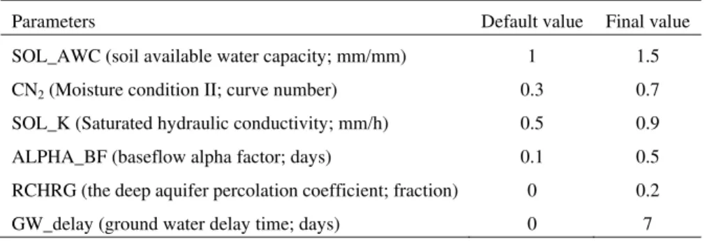
Only those parameters with high and medium sensitivities were considered in the calibration process except
SOL_AWC, CN2, and SOL_K. For SOL_K, the measured values were considered and SOL_AWC was
already adjusted in the process of crop parameters adjustment. The default values and the adjusted values for
IAEES www.iaees.org
0 50 100 150 200 250 300 350 0 0.05 0.1 0.15 0.2 0.25 0.3 0.35 0.4 Precipitation OBScms simulation 0 50 100 150 200 250 300 350 400 450 500 0 0.5 1 1.5 2 2.5 3 3.5 4 4.5 5 precipitation obs (cms) simulation
y = 1.245x + 0.008 R² = 0.689 0.00 0.05 0.10 0.15 0.20 0.25 0.30 0.35 0.40 0.45
0 0.1 0.2 0.3 0.4
Table 2 Default and final parameters values of SWAT used to calibrate streamflow at outlet.
Parameters Default value Final value
SOL_AWC (soil available water capacity; mm/mm)
CN2 (Moisture condition II; curve number)
SOL_K (Saturated hydraulic conductivity; mm/h)
ALPHA_BF (baseflow alpha factor; days)
RCHRG (the deep aquifer percolation coefficient; fraction)
GW_delay (ground water delay time; days)
1 0.3 0.5 0.1 0 0 1.5 0.7 0.9 0.5 0.2 7
SWAT was manually calibrated and the daily simulated and observed streamflows at the HMN-SW outlet were compared to calibration periods (Fig. 4a). Minor discrepancies between the observed and simulated
stream discharges were observed. During the calibration period, the calculated R2 on a daily scale was about
0.69 (Fig. 4b). The monthly simulated and observed streamflows were compared with the precipitation (Fig.
4c). The calculated R2 on a monthly scale was about 0.97 (Fig. 4d) which can be considered as acceptable.
Fig. 4 Daily and monthly observed and simulated streamflows at the HMN-SW outletduring the calibration and the coefficient of
determination (R2) periods.
(a) Daily observed and simulated streamflows
y = 1.511x + 0.105 R² = 0.969 0 0.5 1 1.5 2 2.5 3 3.5 4 4.5
0 1 2 3
(b) The calculated R2 on daily scale
Observed (mg L-1
) Strea mflow (cm s) Precipi ta ti on (mm) Sim u la te d (m g L -1) 1 Strea mflow (cm s) Month
(c) Monthly observed and simulated streamflows (d) The calculated R2 on monthly scale
Precipi ta ti on (mm) Sim u la te d (m g L -1)
Observed (mg L-1
From Fig. 4, it seems that the problem in simulating high peaks flows in SWAT model was occurred when it was implemented in particular climatic conditions of tropical rainforest. In addition, the SWAT
over-estimation of streamflows during high discharges might result from an underover-estimation of the daily precipitations (especially those events corresponding to peak stream discharges) arising from an inadequate
sampling of sub-basin precipitations. Values of R2 greater than 0.8 were also found in several SWAT
hydrological calibration studies (Kalin and Hantush, 2006; Wang and Melesse, 2006; Jha et al., 2007).
3.3 SWAT simulation and assessing on main functions of watershed ecosystem 3.3.1 Water balance
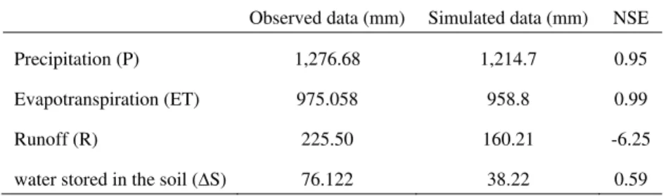
This is considered as the first main functions of watershed ecosystem. Understanding the consequences of land use practices on hydrological processes, such as changes in soil loss, sediment yield and water yield from
altering hydrological processes in terms of precipitation (P), evapotranspiration (ET), runoff (R), and water
stored in the soil (∆S) is prime importance. Many these components water balance is considered to be the first
main function of watershed ecosystem. The result of this function from the field and the SWAT model simulation are shown in Table 3.
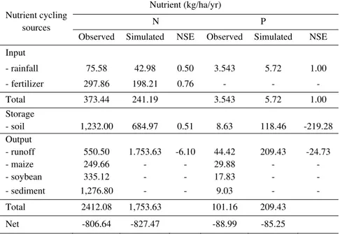
3.3.2 Nutrient balance
The result of nutrient analysis in agricultural watershed ecosystem can be divided into 4 parts are as follow; (1) nutrient into the system (nutrient from rain and fertilizer or mineral), (2) nutrient loss (nutrient in runoff and
harvesting), (3) nutrient storage in soil, and (4) net loss or gain. Only nitrogen (N) and phosphorus (P) can be able to simulation by SWAT model. The result in this study found that nutrient balance (N and P) from the observed value and the simulated value by SWAT model are shown in Table 4.
3.3.2 Nutrient balance
The result of nutrient analysis in agricultural watershed ecosystem can be divided into 4 parts are as follow; (1)
nutrient into the system (nutrient from rain and fertilizer or mineral), (2) nutrient loss (nutrient in runoff and harvesting), (3) nutrient storage in soil, and (4) net loss or gain. Only nitrogen (N) and phosphorus (P) can be able to simulation by SWAT model. The result in this study found that nutrient balance (N and P) from the
observed value and the simulated value by SWAT model are shown in Table 4. 3.3.3 Carbon balance
In this study, soil carbon sequestration was collected from plant (maize and soybean). The result of this function from the field and the SWAT model simulation are shown in Table 5.
3.3.4 Energy balance
Net radiation (Rn) is important to the Bowen ratio-energy balance method which is often used to estimate
latent heat flux (λE). Estimates of latent heat flux and the sensible heat flux (H) were using the yearly sums of
solar radiation (Rs), net radiation (Rn), and Bowen ratio. Rn from the regression formula and the corresponding
values was 67.45%. Rs, λE, and H were 82.25% and 17.75% of Rn, shown in Table 6.
Table 3 Observation and simulation of water balance in the HMN-SW during 2011-2012.
Observed data (mm) Simulated data (mm) NSE
Precipitation (P)
Evapotranspiration (ET)
Runoff (R)
water stored in the soil (∆S)
1,276.68
975.058
225.50
76.122
1,214.7
958.8
160.21
38.22
0.95
0.99
-6.25
IAEES www.iaees.org
Table 4 Net loss or gain of nutrients in agricultural watershed ecosystem at the HMN-SW during 2011-2012.
Nutrient cycling sources
Nutrient (kg/ha/yr)
N P
Observed Simulated NSE Observed Simulated NSE
Input
- rainfall 75.58 42.98 0.50 3.543 5.72 1.00
- fertilizer 297.86 198.21 0.76 - - -
Total 373.44 241.19 3.543 5.72 1.00
Storage
- soil 1,232.00 684.97 0.51 8.63 118.46 -219.28
Output
- runoff 550.50 1.753.63 -6.10 44.42 209.43 -24.73
- maize - soybean 249.66 335.12 - - - - 29.88 17.83 - - - -
- sediment 1,276.80 - - 9.03 - -
Total 2412.08 1,753.63 101.16 209.43
Net -806.64 -827.47 -88.99 -85.25
Remark: Nutrients (+) is mean gain, (-) is mean lost
Table 5 Observation and simulation of carbon balance in the HMN-SW during 2011-2012.
Observed data Simulated data NSE
1. The live microbes to form soil organic matter (SOM)
2. Organic carbon in harvested plant
3. Organic carbon in plant was released back into the
atmosphere through burning
4. Organic carbon in soil was released back into the
atmosphere through burning
34.96% 7.03% 88.31% 9.2% 48.99% 20.57% 93.21% 17.76% 100% 99.84% 100% 99.98%
Table 6 Energy balance in agricultural watershed ecosystem at the HMN-SW during 2011- 2012.
Month Rs
(W/m2)
Rn
(W/m2)
Rs (%)
Bowen ratio
λE
(W/m2)
H
(W/m2)
λE (%)
H (%)
Jan. 412.6 272.6 59.9 0.1 247.8 24.8 90.91 9.09
Feb. 459.81 313.5 59.3 0.2 261.3 52.3 83.33 16.67
Mar. 467.8 309.3 57.4 0.2 257.8 51.6 83.33 16.67
Apr. 522.47 326 57.8 0.2 271.7 54.3 83.33 16.67
May 438.88 304.8 62.9 0.2 254.0 50.8 83.33 16.67
Jun. 402.56 300.1 63.5 0.4 214.4 85.7 71.43 28.57
Jul. 399.05 318 76.1 0.1 289.1 28.9 90.91 9.09
Aug. 374.93 357.2 74.8 0.1 324.7 32.5 90.91 9.09
Sep. 383.55 392.2 81.7 0.2 326.8 65.4 83.33 16.67
Oct. 356.11 353.9 77.4 0.2 294.9 59.0 83.33 16.67
Nov. 333.09 308.5 72.3 0.4 220.4 88.1 71.43 28.57
Dec. 321.01 278.6 66.4 0.4 199.0 79.6 71.43 28.57
Range 417.8-563.9 272.6-392.2 57.4-81.76 0.1-0.4 199.0-326.8 24.8-88.1 71.4-90.9 9.1-28.6
3.4 The e SWAT m HMN-SW sediment watershe 4 Conclu The SW those ob responsib and pho temperat water fro percolati
effect on ma model was ca
W. Simulatio t yields wer
ed ecosystem
Fig. 5 The
usions AT model si served value
ble for this d osphorous lea
tures could ha om rainfall t
on. The flush
ain functions alibrated and
on and asses e generally
in the
HMN-effect on main
imulated valu s. It was spe
discrepancy. I aching durin
ave been low to flow as s hing of nitrog
of watershe applied to si
ssment on m in agreemen
-SW by using
functions of wa
ue of nitroge eculated that
It was also id ng the wet
wer than the a surface runof gen will be de
d ecosystem imulate water
main function nt with the o
g SWAT mod
atershed ecosys
en and water main functio
dentified that season. This
actual temper ff rather than elayed until dr
in the HMN r and sedime
ns of watersh observed dat
del can be illu
stem in the HM
r soluble pho ons of waters
t the model h s study susp
ratures, which n being part ry soils in the
N-SW ent yields, an
hed ecosystem ta. The effec
ustrated in Fig
MN-SW by using
osphorous we hed ecosyste
had difficulti pected that m
h may have c itioned into e dry period.
nd nutrient loa
m in term o ct on main
g. 5.
g SWAT model
ere generally em in tropica
ies in simulat model simul
caused 100% surface runo
adings in the
of water and functions of
l.
y higher than al zones were
ting nitrogen lated ground
IAEES www.iaees.org
The calibrated SWAT model was used to estimate the effect on main functions of watershed ecosystem on water and sediment yields. On an annual basis, under current level of water balance, the effect of water
balance in the HMN-SW during from 2008-2012 was a land slide and erosion due to input was more than output. The results of carbon balance from SWAT model simulation were generally higher than observed values. The organic carbon compounds are used for plant growth and the microbes to form soil organic matter
(SOM) were less than organic carbon in harvesting plant from watershed ecosystem, organic carbon in plant and soil are released back into the atmosphere through burning. From the result, it could be indicated that the
HMN-SW was the carbon source watershed ecosystem, because after maize harvesting the burning process was operated and organic carbon in plant was released to the atmosphere.
Acknowledgement
The authors are gratefully acknowledging the Center for Advanced Studies in Tropical Natural Resources (CASTNR), National Research University-Kasetsart University (NRU-KU) for supporting this research grant.
References
Arnold JG, Srinivasan R, Muttiah RS, et al. 1999. Continental scale simulation of the hydrologic balance. Journal of American Water Resources Association, 35(5): 1037-1051
Arnold JH, Fohrer N. 2005. SWAT2000: Current capabilities and research opportunities in applied watershed modeling. Hydrological Processes, 19: 563-572
Arnold JG, Srinivasan R, Muttiah RS, et al. 1998. Large-area hydrologic modeling and assessment: Part I.
Model development. Journal of American Water Resources Association, 34 (1): 73-89
Bakker MM, Govers G, Kosmas C, et al. 2005. Soil erosion as a driver of land-use change. Agriculture,
Ecosystems & Environment, 105: 467-481
Beasley DB. 1991. ANSWERS User’s Manual Second Edition. Agricultural Engineering Department, University of Georgia, USA
Borah DK, Bera M.2003. Watershed-scale hydrologic and nonpoint-source pollution models: review of mathematical bases. Transanctions of the ASAE, 46(6): 1553-1566
Foley JA. 2005. Global consequences of land use. Science, 309: 570-574
Galloway JN. 2004. Nitrogen cycles: past, present, and future. Biogeochemistry, 70: 153-226
Gassman PW, Reyes MR, Green CH, et al. 2007. The Soil and Water Assessment Tool: historical development,
applications and future research directions. Transactions of the ASABE, 50 (4): 1211-1250
Gitau MW, Gburek WJ, Jarrett AR. 2005. A tool for estimating best management practice effectiveness for
phosphorus pollution control. Journal of Soil and Water Conservation, 60(1): 1-9
Holman IP, Hollis JM, Alavi G, et al. 2001. CAMSCALE-Up scaling Predictive Models and Catchment Water Quality. Draft Final Report to DGXII, Commission of the European Communities under, Contract
ENV4-CT97-0439
Jha M, Gassman PW, Arnold JG. 2007. Water quality modeling for the Raccoon River watershed using
SWAT2000. Transactions of the ASABE, 50(2): 479-493
Kalin L, Hantush M. 2006. Hydrologic modeling of an eastern Pennsylvania watershed with NEXRAD and rain gauge data. Journal of Hydrologic Engineering (ASCE), 11(6): 555-569
Lenhart T, Fohrer N, Frede HG. 2003. Effects of land use changes on the nutrient balance in mesoscale catchments. Physics and Chemistry of the Earth, 28: 1301-1309
Lenhart T, Van Rompaey A, Steegen A, et al. 2005. Considering spatial distribution and deposition of sediment in lumped and semi-distributed models. Hydrological Processes, 19(3): 785-794
Nash JE, Sutcliffe JE. 1970. River flow forecasting through conceptual models: Part 1. A discussion of
principles. Journal of Hydrology, 10(3): 282-290
USDA-SCS. 1972. National Engineering Handbook. United States Department of Agriculture (USDA), Soil
Conservation Service SCS, USA
Van Griensven, Bauwens AW. 2005. Application and evaluation of ESWAT on the Denderbasin and Wister Lake basin. Hydrological Processes, 19 (3): 827-838
Van Liew MW. 2009. Streamflow, sediments and nutrient simulation of the Bitterroot watershed using SWAT. In: Proceedings of the 2009 International SWAT Conference. Boulder, Colorado, USA
Wang X, Melesse AM. 2006. Effects of STATSGO and SSURGO as inputs on SWAT model’s snowmelt simulation. Journal of the American Water Resources Association, 42(5): 1217-1236
Williams JR, Jones CA, Dyke PT. 1984. A modeling approach to determining the relationship between