www.hydrol-earth-syst-sci.net/18/4565/2014/ doi:10.5194/hess-18-4565-2014
© Author(s) 2014. CC Attribution 3.0 License.
Complex networks for streamflow dynamics
B. Sivakumar1,2and F. M. Woldemeskel1
1School of Civil and Environmental Engineering, The University of New South Wales, Sydney, Australia 2Department of Land, Air and Water Resources, University of California, Davis, CA, USA
Correspondence to: B. Sivakumar ([email protected])
Received: 3 June 2014 – Published in Hydrol. Earth Syst. Sci. Discuss.: 2 July 2014 Revised: – – Accepted: 14 October 2014 – Published: 20 November 2014
Abstract. Streamflow modeling is an enormously challeng-ing problem, due to the complex and nonlinear interactions between climate inputs and landscape characteristics over a wide range of spatial and temporal scales. A basic idea in streamflow studies is to establish connections that generally exist, but attempts to identify such connections are largely dictated by the problem at hand and the system components in place. While numerous approaches have been proposed in the literature, our understanding of these connections re-mains far from adequate. The present study introduces the theory of networks, in particular complex networks, to exam-ine the connections in streamflow dynamics, with a partic-ular focus on spatial connections. Monthly streamflow data observed over a period of 52 years from a large network of 639 monitoring stations in the contiguous US are stud-ied. The connections in this streamflow network are exam-ined primarily using the concept of clustering coefficient, which is a measure of local density and quantifies the net-work’s tendency to cluster. The clustering coefficient analy-sis is performed with several different threshold levels, which are based on correlations in streamflow data between the sta-tions. The clustering coefficient values of the 639 stations are used to obtain important information about the connections in the network and their extent, similarity, and differences be-tween stations/regions, and the influence of thresholds. The relationship of the clustering coefficient with the number of links/actual links in the network and the number of neighbors is also addressed. The results clearly indicate the usefulness of the network-based approach for examining connections in streamflow, with important implications for interpolation and extrapolation, classification of catchments, and predictions in ungaged basins.
1 Introduction
Streamflow forms an important input for a wide range of ap-plications in hydrology, water resources, environment, and ecosystem. However, its estimation or prediction is an enor-mously challenging problem, since streamflow arises as a re-sult of complex and nonlinear interactions between climate inputs (external factors) and landscape characteristics (inter-nal factors) that occur over a wide range of spatial and tem-poral scales. For instance, streamflow is governed not only by the distribution of rainfall (in both space and time) but also by the nature and state of the catchment (e.g., topography, vege-tation, soil, geology); see Beven (2006) for a compilation of, and stimulating insight into, some early benchmark studies (1933–1984) on streamflow generation processes. Attempts to monitor, model, and predict streamflow have been a central topic in hydrology during the last century or so; see, for ex-ample, Salas et al. (1995), Grayson and Blöschl (2000), Duan et al. (2003), Mishra and Coulibaly (2009), and Hrachowitz et al. (2013) for comprehensive accounts on streamflow mon-itoring, modeling, and prediction.
same developments have, at times, played an indirect role in creating imbalance and hindering true progress, as they have contributed to the perhaps unnecessary complexifica-tion in models (rather than simplificacomplexifica-tion), highly special-ized conceptual notions that are often suitable only for spe-cific situations (rather than generalization frameworks that suit all conditions), difficult-to-bridge gaps between theory and practice, and lack of communication among researchers as well as between researchers and practitioners; see, for ex-ample, Perrin et al. (2001), Beven (2002), Kirchner (2006), Sivakumar (2008), and Young and Ratto (2009) for some details.
It is important to recognize that a fundamental idea in streamflow (and other hydrologic) studies is to establish con-nections that generally exist between the different elements or items (known or assumed) of the underlying system. De-pending upon the situation (e.g., catchment, purpose, prob-lem), these elements include hydroclimatic variables, catch-ment characteristics, model parameters, and others (and their combinations), and their connections are often different with respect to space, time, and space–time. Unraveling the nature and extent of these connections has always been a great chal-lenge, not to mention the challenge in the identification of all the relevant elements in the first place. Thus far, a plethora of concepts and methods have been proposed and applied for studying the connections associated with streamflow, in-cluding those based on time, distance, correlation, variability, scale, patterns, and many other properties/measures as well as their combinations and variants, in both single-variable and multi-variable perspectives; see, for example, Gupta et al. (1986), Salas et al. (1995), Grayson and Blöschl (2000), Yang et al. (2004), Archfield and Vogel (2010), and Li et al. (2012) for some details. Despite the progress made through these concepts and methods, our understanding of the connections in streamflow is still far from adequate.
In view of this, there is indeed a need to greatly advance our studies on streamflow connections. Some important cur-rent and foreseeable future problems, including our ever-increasing demands for water, the potential impacts of cli-mate change on water security and hydroclimatic disasters, and the numerous issues associated with the management of our environment and ecosystems, further reflect the urgency to this need. A greater understanding of streamflow connec-tions will also enhance our recent and current efforts in the estimation of data at ungaged locations (e.g., predictions in ungaged basins – PUB) (see Hrachowitz et al., 2013) and development of a generalization framework for hydrologic modeling (e.g., catchment classification) (see Sivakumar et al., 2014), among others. The question, however, remains on the identification of a suitable theory that can help bring ad-vancement to studies on streamflow connections. In this re-gard, recent developments in the field of complex systems science can offer some crucial clues. The present study intro-duces the theory of complex networks, or simply networks,
for studying connections in streamflow. In particular, the study focuses on spatial connections in streamflow.
The origin of the concept of networks can be traced back to the works of Leonhard Euler, during the first half of the eigh-teenth century, on the Seven Bridges of Königsberg (Euler, 1741), which laid the foundations of what would become popularly known as graph theory. Graph theory witnessed several important theoretical developments in the nineteenth century, including topology (originally introduced as topolo-gie in German) (Listing, 1848) and trees (Cayley, 1857). Further significant advances were made during the twen-tieth century, especially with the development of random graph theory by Erdös and Rényi (Erdös and Rényi, 1960). The concepts of graph theory, and random graph theory in particular, have found a wide variety of applications in nu-merous fields, including linguistics, physics, chemistry, bi-ology, socibi-ology, engineering, economics, and ecology; see, for example, Berge (1962), Bondy and Murty (1976), and Bollobás (1998) for extensive reviews.
recent study, Sivakumar (2014) has argued that networks can be useful for studying all types of connections in hydrology and, hence, can provide a generic theory for hydrology.
With the encouraging results reported by the above stud-ies, the present study explores the usefulness of the theory of networks for studying connections in streamflow, especially the spatial connections. To this end, monthly streamflow data observed over a period of 52 years (1951–2002) from each of 639 gaging stations in the contiguous US are studied. The connections are examined primarily using the concept of clustering coefficient. The clustering coefficient is a measure of local density and, hence, quantifies the tendency of a net-work to cluster. The implications of the clustering coefficient results for interpolation/extrapolation of streamflow data as well as for classification of catchments are also discussed. To put the clustering coefficient analysis in a proper perspec-tive, traditional linear correlation analysis (Pearson correla-tion coefficient) and another simple network-based analysis (degree centrality) are also performed.
The rest of this paper is organized as follows. Section 2 introduces the concept of networks and describes the proce-dure for calculation of degree centrality and clustering co-efficient in a network. Section 3 presents details of the study area and streamflow data considered. Section 4 reports the re-sults, first from the traditional linear correlation analysis and then from the network-based degree centrality and clustering coefficient analysis. Section 5 highlights the implications of the results.
2 Network and clustering coefficient 2.1 Network
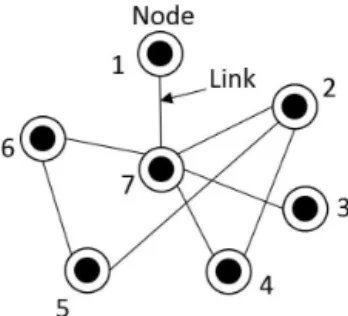
A network or a graph is a set of points connected together by a set of lines, as shown in Fig. 1. The points are referred to as vertices or nodes and the lines are referred to as edges or links; here, the term nodes are used for points and the term links are used for lines. Mathematically, a network can be represented as G= {P , E}, where P is a set of N nodes (P1, P2, . . . , PN) and E is a set of n links. The network shown in Fig. 1 has N=7 (nodes) andn=8 (links), with P = {1,2,3, 4, 5,6,7} and E= {{1,7}, {2,3}, {2,5}, {2, 7},{3, 7},{4,7},{5,6},{6,7}}.
Figure 1 is perhaps the simplest form of network, i.e., one with a set of identical nodes connected by identical links. There are, however, many ways in which networks may be more complex. For instance, a network: (1) may have more than one different type of node and/or link; (2) may contain nodes and links with a variety of properties, such as differ-ent weights for differdiffer-ent nodes and links depending on the strength of nodes and connections; (3) may have links that can be directed (pointing in only one direction), with ei-ther cyclic (i.e., containing closed loops of links) or acyclic form; (4) may have multi-links (i.e., repeated links between
Figure 1. Network in its simplest form, i.e., an undirected network
with only a single type of node and a single type of link.
the same pair of nodes), self-links (i.e., links connecting a node to itself), and hyperlinks (i.e., links connecting more than two nodes together); and (5) may be bipartite, i.e., con-taining nodes of two distinct types, with links running only between unlike types.
There are many different ways and measures to study the characteristics of networks. In the context of the mod-ern theory of complex networks (which also include random graphs), degree centrality, clustering coefficient, small-world networks, and degree distribution are some of the prominent concepts. As the present study uses the concepts of degree centrality and clustering coefficient for studying streamflow connections, they are described next.
2.2 Degree centrality
Centrality is one of the most basic and intuitive measures of a network; see Freeman (1979) for an early comprehensive review. The idea behind the use of centrality as a network measure is that it identifies whether a given node, sayiin a network, is more central or more influential than another node in the network. The degree centrality of nodeiin a net-work ofN nodes is defined as the number of first neighbors (or simply neighbors) of nodeidivided by the total number of possible neighbors (N−1) in the network.
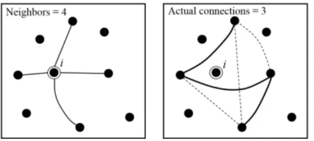
Let us consider a selected nodeiin a network ofNnodes, havingki links which connect it toki other nodes. For illus-tration, Fig. 2 presents a network consisting of nine nodes (i.e., N=9), with the node i having four links (i.e., with four other nodes) (see Fig. 2, left panel). In this case, the four nodes corresponding to the four links are the neigh-bors of nodei, which are identified based on some condi-tions (e.g., correlation between nodeiand other nodes in the network), while the total number of possible neighbors for nodeiis eight (i.e.,N−1).
2.3 Clustering coefficient
Figure 2. Connections in networks and calculation of clustering
co-efficient: nearest neighbors and actual connections.
density. The concept of clustering has its origin in sociol-ogy, under the name fraction of transitive triples (Wasserman and Faust, 1994). The procedure for calculating the cluster-ing coefficient is as follows.
Let us consider first a selected nodeiin the network, hav-ingki links which connect it toki other nodes, as shown in Fig. 2 (left panel). If the neighbors of the original node (i) were part of a cluster, there would be ki(ki−1)/2 links between them. As shown in Fig. 2 (right panel), there are 4(4−1)/2=6 links in the cluster of nodei. The clustering coefficient of node iis then given by the ratio between the numberEi of links that actually exist between thesekinodes (shown as solid lines on Fig. 2, right panel) and the total num-berki(ki−1)/2 (i.e., all lines on Fig. 2, right panel), Ci=
2Ei ki(ki−1)
. (1)
The clustering coefficient of the whole networkCis the av-erage of the clustering coefficientsCi’s of all the individual nodes.
The clustering coefficient of a random graph is C=p (where pis the probability of two nodes being connected), since the links in a random graph are distributed randomly. However, the clustering coefficient of real networks is gen-erally much larger than that of a comparable random net-work (i.e., having the same number of nodes and links as the real network). Therefore, the clustering coefficient analy-sis offers useful information about the nature of the network and, hence, the appropriate model (e.g., level of complexity), among others.
3 Study area and data
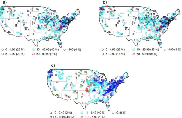
In the present study, streamflow data from the US are stud-ied to explore the usefulness of the theory of networks for identifying connections in streamflow, with a focus on spatial connections. Monthly data from an extensive network of 639 streamflow gaging stations in the contiguous US are studied. The locations of these 639 stations are shown in Fig. 3. The above streamflow data are obtained from the US Geologi-cal Survey database, in particular from the Hydro-Climatic Data Network (HCDN), originally developed by Slack and
Landwehr (1992) and subsequently updated at different times, with the last update in 2009; see Lins (2012) for details (http://water.usgs.gov/osw/hcdn-2009/). The HCDN is a sub-set of all USGS (United States Geological Survey) stream-gages for which the streamflow primarily reflects prevailing meteorological conditions for specified years; see Kiang et al. (2013) for the latest and comprehensive account of USGS streamflow gages across the entire US. The HCDN stream-gage stations were screened to exclude sites where human activities, such as artificial diversions, storage, and other ac-tivities in the drainage basin or the stream channel, affect the natural flow of the watercourse.
Streamflow data in the US are commonly expressed in water years, which commence in October. The data used in this study are those observed over a period of 52 years (1951–2002), obtained from an earlier version of HCDN. The data are average monthly values (not anomalies). During the past few decades, a large number of studies have investi-gated the above streamflow data set (or a part or variant of it) in many different contexts (e.g., Slack and Landwehr, 1992; Kahya and Dracup, 1993; Vogel and Sankarasubramanian, 2000; Sivakumar, 2003; Tootle and Piechota, 2006; Patil and Stieglitz, 2012; Sivakumar and Singh, 2012; Kiang et al., 2013). Some of these studies have explicitly addressed the connections of streamflow between the stations, includ-ing in the context of data correlations, catchment similari-ties, and other measures; see, Patil and Stieglitz (2012) and Kiang et al. (2013) for some recent studies. Many studies have explored the connections of streamflow with large-scale climatic patterns and relevant indexes, including El Niño, La Niña, Southern Oscillation Index, Pacific North Amer-ica Index, and Pacific Decadal Oscillation. However, within the specific context of the network analysis for connections among streamflow stations presented here, as well as in the broader context of complex systems science for streamflow analysis, the studies by Sivakumar (2003) and Sivakumar and Singh (2012) are worth mentioning, as they have ad-dressed the aspects of streamflow variability, nonlinearity, and dominant governing mechanisms, especially for stud-ies on model simplification, data interpolation/extrapolation, and catchment classification framework.
Figure 3. Characteristics of monthly streamflow observed at 639 stations in the US: (a) mean, (b) standard deviation, and (c) coefficient of
variation.
flow characteristics can play important roles in the nature and extent of connections in streamflow between the different sta-tions. While studying their influences is clearly important, the present study does not specifically attempt to address this. Rather, the focus of the present study is in identifying the ex-tent of connections among the stations based on streamflow data alone.
4 Analysis and results
The usefulness of the theory of networks for studying con-nections in streamflow is examined primarily through the clustering coefficient analysis on the monthly streamflow data from the above 639 stations in the US. To put the clustering coefficient analysis in a proper perspective, how-ever, linear correlation and degree centrality analyses are also performed.
4.1 Linear correlation analysis
A common approach to examine connections between streamflow observed at different stations is through a sim-ple linear cross correlation analysis, where the correlation for any given station is given by the average of its corre-lation with all the other stations. Several variants of this procedure are also usually considered. These include: near-est neighbors – for example, number of nearby stations based on distance or stations within a pre-defined region of
geographicproximity or neighborhood, with equal or unequal weight age (e.g., inverse distance); and similar stations – sta-tions with similar properties (e.g., in terms of climate, rain-fall, basin characteristics, land use), which may or may not include nearest stations. These and many other correlation-based procedures (e.g., spline fitting) are routinely employed for interpolation and extrapolation of streamflow and other hydrologic data.
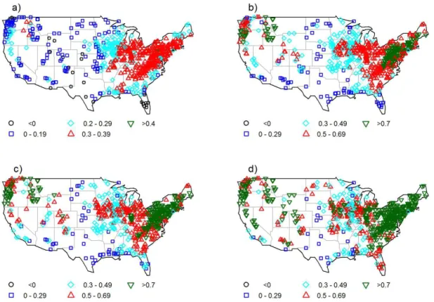
Figure 4. Linear correlation for streamflow: average of correlation with (a) all 638 stations, (b) nearest 30 neighbors, (c) nearest 15 neighbors,
and (d) nearest 5 neighbors.
finer timescales through the central limit theorem (Anderson, 2010).
When all the 638 stations are considered, the correlation values are generally very low, as expected, with only 0.5 % of the stations exceeding a value of 0.4 (see Fig. 4a). This is mainly due to the consideration of a very large region, with the stations coming from different climatic, catchment, land use, and other characteristics. When the number of sta-tions is reduced, the results get generally better – see Fig. 4b (30 neighbors), Fig. 4c (15 neighbors), and Fig. 4d (5 neigh-bors). Among the three neighborhood cases, the best correla-tion results are obtained when the neighborhood is the small-est, i.e., 5 neighbors (Fig. 4d), with a large number of stations having correlations above 0.7.
While one can study a large number of combinations in terms of the neighborhood, what is evident from even the very few cases presented here is that there are obvious re-gional patterns in terms of correlations, regardless of the number of neighbors. These regional patterns are considered to have important implications for a wide range of studies in hydrology and water resources, as they are commonly used as a basis for interpolation and extrapolation of streamflow and, subsequently, for water resources assessment, planning, and management. However, as Sivakumar and Singh (2012) point out, through their nonlinear dynamic study on stream-flow data from the western US, the use of regional patterns as basis for streamflow studies may be misleading, as such
patterns are not necessarily a true representation of the ac-tual connections between the stations but may just be spuri-ous. The obvious question, therefore, is how to identify if the connections are actual or spurious? This is where the ideas from the theory of networks can be particularly useful. 4.2 Degree centrality analysis
The degree centrality is calculated for the monthly stream-flow data from the network of 639 stations in the US, ac-cording to the procedure described in Sect. 2.2. The essence of the procedure for the streamflow data is as follows. For a given streamflow station or nodei, the nearest neighborskiin the network of 639 stations (more specifically, the remaining 638 stations) are identified based on a (pre-specified) thresh-old value (T). To define the threshold value, the correlations in streamflow data between different stations are considered as a reasonable measure. With this, if, for example, the cor-relation between stationiand any other station(s) in the en-tire network of 639 stations exceeds the threshold value, then that station(s) will be considered as a neighbor(s),ki, for sta-tioni. The degree centrality of stationiis then given by the ratio of the number of neighbors to the total number of pos-sible neighbors (i.e., 638).
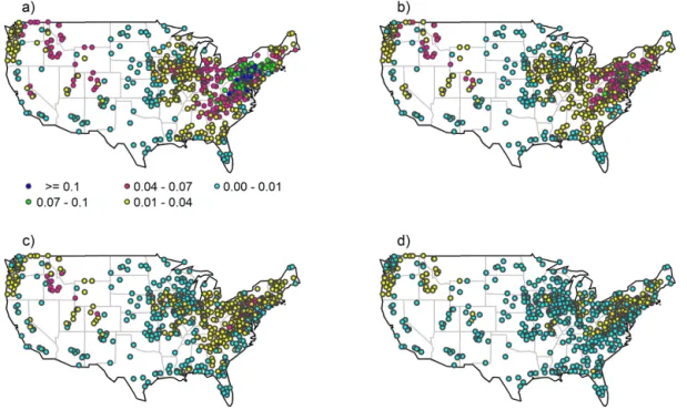
Figure 5. Degree centrality for four correlation thresholds: (a) 0.70, (b) 0.75, (c) 0.80, and (d) 0.85.
values for streamflow (and other hydrologic) data, our expe-rience in streamflow studies, especially spatial and temporal correlations, offers some useful clues. For instance, stream-flow data generally exhibit high spatial correlations (when compared to rainfall values, for example), especially at the monthly scale. With this knowledge, and also with the con-dition that−1≤T ≤1.0, closer intervals of values are con-sidered at the higher end of correlations and vice versa. In addition, very low values (say,T <0.30) and very high val-ues (say,T >0.85) do not offer much help in the analysis; for instance,T <0.30 normally results in a very large num-ber of neighbors, whileT >0.85 results in a very small num-ber. Considering all these, eight threshold values are used for analysis: 0.30, 0.40, 0.50, 0.60, 0.70, 0.75, 0.80, and 0.85.
Figure 5a–d, for example, show the results from the de-gree centrality analysis for the 639 stations for threshold val-ues of 0.70, 0.75, 0.80, and 0.85. The results offer some in-teresting observations. For instance, only a very small num-ber of streamflow stations (blue circles) have connections with more than 10 % of the other stations in the network of 639 stations, while a large number of stations (cyan circles) have connections to less than just 1 % of the other stations. Indeed, for thresholds of 0.70, 0.75, 0.80, and 0.85, the num-ber of stations having connections with more than 10 % of the stations is only 39, 0, 0, and 0, respectively, while the num-ber of stations having connections with less than 1 % of the stations is 118, 160, 257, and 429, respectively. This clearly suggests that only a small proportion of stations has consid-erable influence in the network, while a large proportion of stations has only very little or almost no influence. This result has significant implications, for example, in interpolation and
extrapolation, especially from the viewpoint of dominant sta-tions (as is the case of 639 stasta-tions forT =0.70; Fig. 5a). It is also important to note, however, that not all of the stations (i.e., neighbors) that a given station has connection with (see Fig. 5a–d) are the geographic neighbors, and some are over long geographic distances (see Sect. 4.3 for further details on this). These observations seem to suggest that the stream-flow network of 639 stations is neither a completely ordered network nor a random graph, but some other.
4.3 Clustering coefficient analysis
Following the description in Sect. 2.3, the procedure for the calculation of the clustering coefficient for the monthly streamflow data from the network of 639 stations in the US is as follows. For a given streamflow station or nodei, the near-est neighborski in the network of 639 stations are identified based on a (pre-specified) threshold value (T), as explained above. The cluster of theseki neighbors then forms the ba-sis for identifying the actual connections. Therefore, the ac-tual connections are those links in the cluster of stations (not just nearest stations) having correlations among themselves exceeding the threshold value. Similar to the degree central-ity analysis above, eight threshold values are considered in the cluster coefficient analysis as well: 0.30, 0.40, 0.50, 0.60, 0.70, 0.75, 0.80, and 0.85.
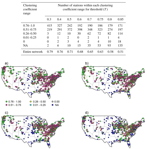
Table 1. Clustering coefficient values for monthly streamflow data from the US.
Clustering Number of stations within each clustering coefficient coefficient range for threshold (T) range
0.3 0.4 0.5 0.6 0.7 0.75 0.8 0.85
0.76–1.0 415 327 242 192 190 186 179 171
0.51–0.75 219 291 372 398 348 323 274 197
0.26–0.50 3 12 10 30 62 72 82 114
0.01–0.25 0 1 2 0 2 1 1 4
0 0 2 3 4 2 4 10 18
NA 2 6 10 15 35 53 93 135
Entire network 0.79 0.76 0.71 0.68 0.65 0.63 0.58 0.51
Figure 6. Clustering coefficients for four correlation thresholds: (a) 0.70, (b) 0.75, (c) 0.80, and (d) 0.85. The six ranges are chosen for better
visualization of results.
values are grouped into six different ranges. In Fig. 6 and Table 1, a clustering coefficient of 0.0 indicates that there are no actual connections, while NA indicates there are no nearest neighbors. From an overall perspective, the cluster-ing coefficient results indicate certain similarity at some sta-tions/regions but significant differences at others. They also offer some specific observations:
– Even nearest stations have significantly different char-acteristics (e.g., connections), as part of a network. Some stations have very strong connections, while oth-ers have almost no or only very weak connections. For instance, the few geographically closer stations in Florida in the southeast region are an excellent example. These few stations have clustering coefficient values
varying anywhere from 0 to 1.0, especially forT=0.7 and 0.75 (Fig. 6a and b).
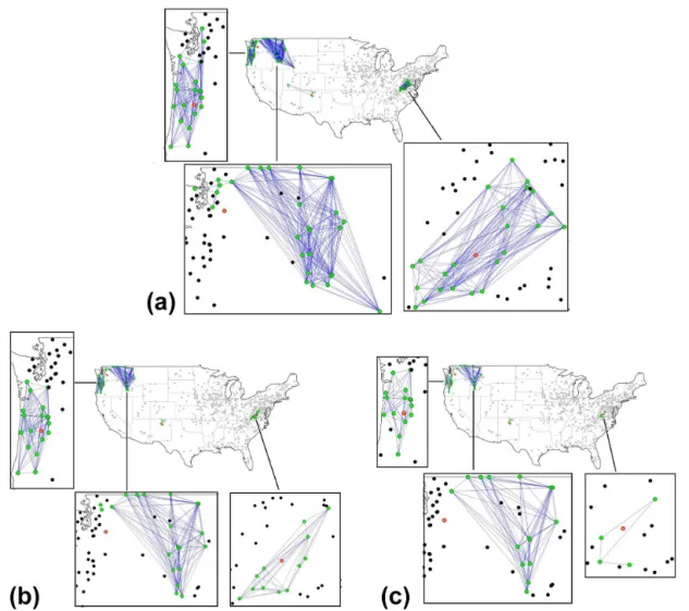
Figure 7. Links in streamflow network for threshold (a)T=0.75; (b)T=0.80; and (c)T=0.85. Four nodes (stations) are chosen for better visualization.
values; see the deep pink circles (Ci=0.51–0.75) and blue circles (Ci=NA).
– There are significant changes in characteristics with re-spect to the threshold values. For instance, as can be seen from Fig. 6 and Table 1, for threshold values of 0.7 and 0.85, the number of stations falling within the clus-tering coefficient range of 0.51–0.75 is 348 and 197, respectively. Indeed, in some cases, further breakdown in the range of clustering coefficient values indicate an even wider difference in the (percentage) number of sta-tions for these thresholds.
– Although there are changes in the number of stations having similar clustering coefficient values with respect to thresholds, there is no consistency in the trend of changes (see, for example, the number of stations falling within the clustering coefficient range of 0.51–0.75). While the usefulness of the clustering coefficient values in assessing connections between streamflow stations and iden-tifying regions having similarity/differences is abundantly
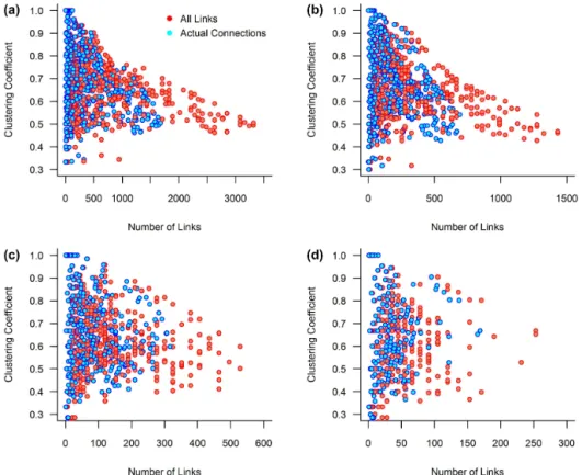
Figure 8. Relationship between clustering coefficient and number of links: (a)T=0.70, (b)T=0.75, (c)T=0.80, and (d)T=0.85. Both all links (red circles) and actual links (blue circles) are presented.
differentconnectivitycharacteristics, for example, for thresh-old level 0.85 (Fig. 7c), with one showing all the actual con-nections within a small neighborhood (see the enlarged plot on the top left) while the other showing no clear neighbor-hood for connectivity (see the enlarged plot on the bottom left). The latter station (see bottom left) is an even more cu-rious case, as most of the neighbors of this station seem to be beyond its (perceived) circle of geographic influence. The actual links observed for the other threshold values also sup-port the above observations.
These observations clearly suggest that our usual approach with consideration of geographic proximity, nearest neigh-bors, regional patterns, and linear correlation-based tech-niques for studying connections in streamflow may have se-rious limitations. Clustering coefficient, and other network-based techniques, offers a better means to examine stream-flow connections. In what follows, we explore the clustering coefficient results even further.
As the clustering coefficient of a network is based on the actual links among all links in the cluster of neighbors of a node (rather than just the links between a node and its neigh-bors), it would be interesting to see how it changes with re-spect to all links and actual links. To this end, Fig. 8a–d show the clustering coefficient values against the number of all links (red circles) and the number of actual links (blue cir-cles) for threshold values of 0.70, 0.75, 0.80, and 0.85 for the
monthly streamflow data from the US. The results lead to the following major observations:
– In general, regardless of the threshold value, there is an inverse relationship between the clustering coefficient and number of links (both for all links and actual links), i.e., higher clustering coefficient for smaller number of links and vice versa.
– The inverse relationship between the clustering coeffi-cient and number of links is generally more evident for lower thresholds (see Fig. 8a and b) when compared to higher thresholds (see Fig. 8c and d). When the thresh-old is very high (T =0.85), this relationship seems to cease to exist.
– The clustering coefficient is generally far more sensitive when the number of links is smaller (see the significant larger spread of circles on theyaxis), but has only very little or almost no sensitivity for a larger number of links (see the very narrow spread followed by a tapering to-wards a fixed value – especially in Fig. 8a and b). Fur-ther, larger numbers of links almost always give lower clustering coefficients.
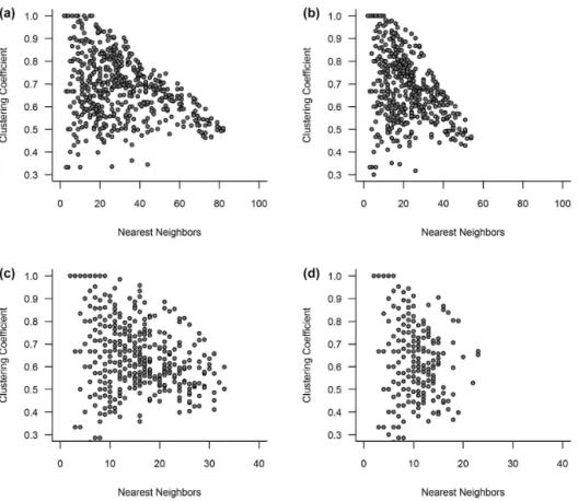
Figure 9. Relationship between clustering coefficient and number of nearest neighbors: (a) T=0.70, (b) T=0.75, (c)T=0.80, and
(d)T=0.85.
Another useful way to look at the clustering coefficient of a network is its relationship with the number of neighbors (ki), which is defined by the threshold value and dictates the (number of) links and actual links. Figure 9a–d show the re-lationship between the clustering coefficient values and the number of neighbors for threshold values of 0.70, 0.75, 0.80, and 0.85 for the monthly streamflow data. The results gen-erally indicate an inverse relationship between the clustering coefficient and number of neighbors, but such a relationship is far more evident for lower threshold values (see Fig. 9a and b) than that for higher threshold values (see Fig. 9c and d). Again, the clustering coefficient is generally far more sensitive when the number of neighbors is smaller (see the larger spread towards the left), but becomes less sensitive for a larger number of neighbors (see the narrow spread towards the right). These observations are somewhat consistent with those made in regard to the number of links (Fig. 8). It is important to recall, however, that the neighbors are not nec-essarily geographic but defined by the threshold values (as shown in Fig. 7).
While these results and observations are still preliminary in nature, they seem to suggest that there is a particular threshold value or range beyond which the inverse relation-ship between the clustering coefficient and number of neigh-bors/links/actual links in the streamflow network may not
hold well for monthly streamflow data from the US, and streamflow data in general.
5 Study implications
One of the basic requirements in studying streamflow dy-namics is to identify connections in space or time or space–time, depending upon the purpose. Although a wide variety of approaches have been developed and applied to identify connections in streamflow dynamics, there is no question that significant improvements are still needed. In this regard, modern developments in the field of network the-ory, especially complex networks, offer new avenues, both for their generality about systems and for their holistic per-spective about connections.
The present study has made an initial attempt to apply the ideas developed in the field of complex networks to examine connections in streamflow dynamics, with particular focus on spatial connections. Application of the concept of clustering coefficient, which is a measure of local density and quanti-fies the tendency of a network to cluster, to monthly stream-flow data from a large network of 639 monitoring stations in the contiguous US, has offered some very interesting results. The clustering coefficient values for the 639 stations suggest that (1) even nearest stations can have significantly different connections and distant stations can have significantly simi-lar connections; (2) connections can be significantly different for different threshold levels; (3) there is generally an inverse relationship between the clustering coefficient and number of neighbors, number of all links, and actual links (in the clus-ter of neighbors); (4) the clusclus-tering coefficient is far more sensitive when the number of neighbors/number of links is smaller, but has only little or no sensitivity when the latter is larger; and (5) the high clustering coefficient value obtained for the entire network is not consistent with the one expected for a random graph, suggesting that the streamflow network is likely to be small-world or scale-free or some other type. The results from the degree centrality analysis suggest that a very small number of streamflow stations have more in-fluence in the network of 639 stations with connections to more than 10 % of the other stations, while a large number of stations have very little influence with connections to just less than 1 % of the other stations. These observations seem to further eliminate the possibility of random nature of the streamflow monitoring network.
Although the present results are preliminary, they offer im-portant information about the connections that possibly exist in the streamflow network, and especially their extent. The clustering coefficient values, and the actual links, are particu-larly useful in the identification of the specific regions where interpolation and extrapolation of streamflow data may be more effective and also of the specific stations whose data can be more reliable for such purposes. For instance, re-gions consisting of stations with high clustering coefficient values would generally provide a more accurate estimation of streamflow when interpolation and extrapolation schemes are employed. It is also important to emphasize, however, that such a region is identified based on cluster of actual
connections, rather than based on our traditional way of geographic proximity, nearest neighbors, regional patterns, and linear correlations. The clustering coefficient values can also offer important clues and guidelines as to the setting up/removal of streamflow monitoring stations in a region. For instance, if a region consists of stations with very high clustering coefficients, then installing additional monitoring stations will not offer any significant benefits. Indeed, one or more monitoring stations from such a region may be re-moved and the resources can be used in regions where ad-ditional stations might offer greater benefits (e.g., in regions where the clustering coefficient values are low). The iden-tification of stations that play more influential roles in the network, as is reflected by the degree centrality results, can also be useful in identifying stations/regions around which interpolation/extrapolation might work better.
Finally, the present study and the results obtained have im-portant implications for a wide range of issues and associ-ated efforts in streamflow modeling, and hydrologic model-ing in general. Among these are (1) PUB, where approaches based on nearest neighbors, regionalization, similarity, and other concepts are commonly adopted; (2) formulation of a catchment classification framework, for simplification and generalization in our modeling paradigm and better com-munication among/between researchers and practitioners; and (3) development of an integrated framework for water planning and management, including in studies on climate change impacts on water resources, that involves proper con-sideration and inclusion of stakeholders and concepts from a vast number of disciplines, including climate, hydrology, engineering, environment, ecology, social sciences, political sciences, economics, and psychology. In view of these, ideas gained from the modern theory of complex networks, and network theory at large, seem to have immense potential in hydrology and water resources.
Acknowledgements. Support for this work was provided by the Australian Research Council (ARC). Bellie Sivakumar ac-knowledges the financial support from ARC through the Future Fellowship grant (FT110100328). We thank the two reviewers, Stefania Scarsoglio and Stacey Archfield, for their constructive comments/suggestions, which have helped improve the quality and presentation of our work further.
Edited by: F. Laio
Reviewed by: S. Scarsoglio and S. A. Archfield
References
Albert, R., Jeong, H., and Barabasi, A.-L.: Internet: Diameter of the world wide web, Nature, 401, 130–131, 1999.
Archfield, S. A. and Vogel, R. M.: Map correlation method: Se-lection of a reference streamgage to estimate daily stream-flow at ungaged catchments, Water Resour. Res., 46, W10513, doi:10.1029/2009WR008481, 2010.
Barabási, A.-L. and Albert, R.: Emergence of scaling in random networks, Science, 286, 509–512, 1999.
Berge, C.: The Theory of Graphs and Its Applications, Matheun, Ann Arbor, MI, USA, 1962.
Beven, K. J.: Uncertainty and the detection of structural change in models of environmental systems, in: Environmental Foresight and Models: a Manifesto, edited by: Beck, M. B., Elsevier Sci-ence Ltd, Oxford, UK, 227–250, 2002.
Beven, K. J.: Benchmark papers in Streamflow Generation Pro-cesses, IAHS Press, Wallingford, UK, 2006.
Boers, N., Bookhagen, B., Marwan, N., Kurths, J., and Marengo, J.: Complex networks identify spatial patterns of extreme rainfall events of the South American Monsoon System, Geophys. Res. Lett., 40, 4386–4392, doi:10.1002/grl.50681, 2013.
Bollobás, B.: Modern Graph Theory, Springer, New York, USA, 1998.
Bondy, J. A. and Murty, U. S. R.: Graph Theory with Applications, Elsevier Science Ltd, New York, USA, 1976.
Bouchaud, J.-P. and Mézard, M.: Wealth condensation in a simple model of economy, Physica A, 282, 536–540, 2000.
Cayley, A.: On the theory of the analytical forms called trees, Phi-los. Mag., 13, 172–176, 1857.
Dalin, C., Konar, M., Hanasaki, N., Rinaldo, A., and Rodriguez-Iturbe, I.: Evolution of the global virtual water trade network, P. Natl. Acad. Sci. USA, 109, 5989–5994, 2012.
Davis, K. F., D’Odorico, P., Laio, F., and Ridolfi, L.: Global spatio-temporal patterns in human migration: A complex network perspective, PLoS ONE, 8, e53723, doi:10.1371/journal.pone.0053723, 2013.
Duan, Q., Gupta, H. V., Sorooshian, S., Rousseau, A. N., and Tur-cotte, R.: Calibration of Watershed Models, in: Water Science and Application Series, vol. 6, American Geophysical Union, Washington, D.C., USA, 2003.
Erdös, P. and Rényi, A.: On the evolution of random graphs, Publ. Math. Inst. Hung. Acad. Sci., 5, 17–61, 1960.
Euler, L.: Solutio problematis ad geometriam situs pertinentis, Comment. Acad. Sci. Petropolitanae, 8, 128–140, 1741. Freeman, L. C.: Centrality in social networks: conceptual
clarifica-tion, Social Netw., 1, 215–239, 1978/79.
Girvan, M. and Newman, M. E. J.: Community structure in so-cial and biological networks, P. Natl. Acad. Sci. USA, 99, 7821–7826, 2002.
Grayson, R. B. and Blöschl, G.: Spatial Patterns in Catchment Hydrology: Observations and Modeling, Cambridge University Press, Cambridge, UK, 2000.
Gupta, V. K., Rodriguez-Iturbe, I., and Wood, E. F.: Scale Prob-lems in Hydrology: Runoff Generation and Basin Response, Wa-ter Science and Technology Library Series, Springer, Dordrecht, the Netherlands, 1986.
Hrachowitz, M., Savenije, H. H. G., Blöschl, G., McDonnell, J. J., Sivapalan, M., Pomeroy, J. W., Arheimer, B., Blume, T., Clark, M. P., Ehret, U., Fenicia, F., Freer, J. E., Gelfan, A., Gupta, H. V., Hughes, D. A., Hut, R. W., Montanari, A., Pande, S., Tet-zlaff, D., Troch, P. A., Uhlenbrook, S., Wagener, T., Winsemius, H. C., Woods, R. A., Zehe, E., and Cudennec, C.: A decade of
predictions in ungaged basins (PUB) – a review, Hydrolog. Sci. J., 58, 1198–1255, 2013.
Kahya, E. and Dracup, J. A.: U.S. streamflow patterns in relation to the El Niño/Southern Oscillation, Water Resour. Res., 29, 2491–2503, 1993.
Kiang, J. E., Stewart, D. W., Archfield, S. A., Osborne, E. B., and Eng., K.: A national streamflow network gap analysis, US Ge-ological Survey Scientific Investigations Report 2013-5013, Re-ston, Virginia, USA, 2013.
Kirchner, J. W.: Getting the right answers for the right rea-sons: Linking measurements, analyses, and models to advance the science of hydrology, Water Resour. Res., 42, W03S04, doi:10.1029/2005WR004362, 2006.
Li, C., Singh, V. P., and Mishra, A. K.: Entropy theory-based cri-terion for hydrometric network evaluation and design: maxi-mum information minimaxi-mum redundancy, Water Resour. Res., 48, W05521, doi:10.1029/2011WR011251, 2012.
Liljeros, F., Edling, C., Amaral, L. N., Stanley, H. E., and Åberg, Y.: The web of human sexual contacts, Nature, 411, 907–908, 2001. Lins, H. F.: USGS Hydro-climatic data network 2009 (HCDN–2009), US Geological Survey Fact Sheet 2012-3047, US Geological Survey, Reston, VA, USA, 2012.
Listing, J. B.: Vorstudien zur Topologie, Vandenhoeck und Ruprecht, Göttingen, Germany, 811–875, 1848.
Milo, R., Shen-Orr, S., Itzkovitz, S., Kashtan, N., Chklovskii, D., and Alon, U.: Network motifs: simple building blocks of com-plex networks, Science, 298, 824–827, 2002.
Mishra, A. K. and Coulibaly, P.: Developments in hydromet-ric network design: a review, Rev. Geophys., 47, RG2001, doi:10.1029/2007RG000243, 2009.
Newman, M. E. J.: The structure of scientific collaboration net-works, P. Nat. Acad. Sci. USA, 98, 404–409, 2001.
Patil, S. and Stieglitz, M.: Controls on hydrologic similarity: role of nearby gauged catchments for prediction at an ungauged catch-ment, Hydrol. Earth Syst. Sci., 16, 551–562, doi:10.5194/hess-16-551-2012, 2012.
Perrin, C., Michel, C., and Andréassian, V.: Does a large number of parameters enhance model performance? Comparative assess-ment of common catchassess-ment model structures on 429 catchassess-ments, J. Hydrol., 242, 275–301, 2001.
Rinaldo, A., Banavar, J. R., and Maritan, A.: Trees, net-works, and hydrology, Water Resour. Res., 42, W06D07, doi:10.1029/2005WR004108, 2006.
Salas, J. D., Delleur, J. W., Yevjevich, V., and Lane, W. L.: Applied Modeling of Hydrologic Time Series, Water Resources Publica-tions, Littleton, Colorado, USA, 1995.
Scarsoglio, S., Laio, F., and Ridolfi, L.: Climate dynamics: A network-based approach for the analysis of global precipita-tion, PLoS ONE, 8, e71129, doi:10.1371/journal.pone.0071129, 2013.
Sivakumar, B.: Forecasting monthly streamflow dynamics in the western United States: a nonlinear dynamical approach, Environ. Modell. Softw., 18, 721–728, 2003.
Sivakumar, B.: Chaos theory for modeling environmental systems: Philosophy and pragmatism, edited by: Wang, L. and Garnier, H., System Identification, Environmental Modelling, and Control System Design, Springer-Verlag, London, 533–555, 2011. Sivakumar, B.: Networks: a generic theory for hydrology?, Stoch.
Environ. Res. Risk Assess., doi:10.1007/s00477-014-0902-7, in press, 2014.
Sivakumar, B. and Singh, V. P.: Hydrologic system complex-ity and nonlinear dynamic concepts for a catchment classi-fication framework, Hydrol. Earth Syst. Sci., 16, 4119–4131, doi:10.5194/hess-16-4119-2012, 2012.
Sivakumar, B., Singh, V. P., Berndtsson, R., and Khan, S. K.: Catchment classification framework in hydrology: challenges and directions, J. Hydrol. Eng., doi:10.1061/(ASCE)HE.1943-5584.0000837, in press, 2014.
Slack, J. R. and Landwehr, V. M.: Hydro-climatic data network (HCDN): a US Geological Survey streamflow data set for the United States for the study of climate variations, 1847–1988, US Geological Survey Open File Report 92-129, US Geological Survey, Reston, Virginia, USA, 1992.
Suweis, S., Konar, M., Dalin, C., Hanasaki, N., Rinaldo, A., and Rodriguez-Iturbe, I.: Structure and controls of the global vir-tual water trade network, Geophys. Res. Lett., 38, L10403, doi:10.1029/2011GL046837, 2011.
Tootle, G. A. and Piechota, T. C.: Relationships between Pacific and Atlantic ocean sea surface temperatures and U.S. streamflow variability, Water Resour. Res., 42, W07411, doi:10.1029/2005WR004184, 2006.
Tsonis, A. A. and Roebber, P. J.: The architecture of the climate network, Physica A, 333, 497–504, 2004.
Vogel, R. M. and Sankarasubramanian, A.: Spatial scaling proper-ties of annual streamflow in the United States, Hydrolog. Sci. J., 45, 465–476, 2000.
Wasserman, S. and Faust, K.: Social Network Analysis, Cambridge University Press, Cambridge, UK, 1994.
Watts, D. J. and Strogatz, S. H.: Collective dynamics of ’small-world’ networks, Nature, 393, 440–442, 1998.
Yang, D., Li, C., Hu, H., Lei, Z., Yang, S., Kusuda, T., Koike, T., and Musiake, K.: Analysis of water resources variabil-ity in the Yellow River of China during the last half cen-tury using historical data, Water Resour. Res., 40, W06502, doi:10.1029/2003WR002763, 2004.