Effective buoyancy ratio: a new parameter to characterize thermo-chemical mixing in the Earth's mantle

(1)

SED

6, 2675–2697, 2014

Effective buoyancy ratio

A. Galsa et al.

Title Page

Abstract Introduction

Conclusions References

Tables Figures

◭ ◮

Back Close

Full Screen / Esc

Printer-friendly Version

Interactive Discussion

Discussion

P

a

per

|

Discus

sion

P

a

per

|

Discussion

P

a

per

|

Discussion

P

a

per

|

Solid Earth Discuss., 6, 2675–2697, 2014 www.solid-earth-discuss.net/6/2675/2014/ doi:10.5194/sed-6-2675-2014

This discussion paper is/has been under review for the journal Solid Earth (SE). Please refer to the corresponding final paper in SE if available.

E

_ff

ective buoyancy ratio: a new parameter

to characterize thermo-chemical mixing in

the Earth’s mantle

A. Galsa, M. Herein, L. Lenkey, M. P. Farkas, and G. Taller

Department of Geophysics and Space Sciences, Eötvös Loránd University, Budapest, Hungary

Received: 28 July 2014 – Accepted: 1 August 2014 – Published: 1 September 2014

Correspondence to: A. Galsa (gali@pangea.elte.hu)

(2)

SED

6, 2675–2697, 2014

A. Galsa et al.

Title Page

Tables Figures

◭ ◮

Back Close

Full Screen / Esc

Discussion

P

a

per

|

Discus

sion

P

a

per

|

Discussion

P

a

per

|

Discussion

P

a

per

|

Abstract

Numerical modeling has been carried out in a 2-D cylindrical shell domain to quan-tify the evolution of a primordial dense layer around the core mantle boundary. Eﬀ ec-tive buoyancy ratio,Beﬀ was introduced to characterize the evolution of the two-layer

thermo-chemical convection in the Earth’s mantle.Beﬀ decreases with time due to (1) 5

warming the compositionally dense layer, (2) cooling the overlying mantle, (3) erod-ing the dense layer by thermal convection in the overlyerod-ing mantle, and (4) diluterod-ing the dense layer by inner convection. WhenBeff reaches the instability point,Beff=1, eff

ec-tive thermo-chemical convection starts, and the mantle will be mixed (Beﬀ=0) during

a short time. A parabolic relation was revealed between the initial density diﬀerence of

10

the layers and the mixing time. Morphology of large low shear velocity provinces as well as results from seismic tomography and normal mode data suggest a value ofBeﬀ≥1

for the mantle.

1 Introduction

The most prominent feature of the lowermost part of the Earth’s mantle is the two

seis-15

mically slow domains beneath Pacific and Africa (e.g. Dziewonski et al., 1993; Garnero et al., 2007a). The nearly antipodal large low shear velocity provinces (LLSVPs) are characterized by −2 to −4 % shear wave and −1 to −2 % pressure wave anomaly, several thousand kilometers lateral extent and 800–1000 km elevation from the core mantle boundary (CMB) (Mégnin and Romanowicz, 2000; Masters et al., 2000; Lay,

20

2005; Zhao, 2009). The margins of the anomalies, where the lateral shear wave veloc-ity gradients are the most pronounced, have sharp sides (Ni et al., 2002; Wang and Wen, 2004; Ford et al., 2006; Garnero and McNamara, 2008) and correlate with hot spot volcanism (Thorne et al., 2004; Torsvik et al., 2010). The existence and the mor-phology of LLSVPs cannot be satisfactorily explained by the variation in temperature,

25

(3)

accumu-SED

6, 2675–2697, 2014

A. Galsa et al.

Title Page

Tables Figures

◭ ◮

Back Close

Full Screen / Esc

Discussion

P

a

per

|

Discus

sion

P

a

per

|

Discussion

P

a

per

|

Discussion

P

a

per

|

lated above the CMB is necessary in a consistent mantle model (Trampert et al., 2004; Ishi and Tromp, 2004; Garnero et al., 2007b; Bull et al., 2009).

A compositionally dense layer around the core is expected to hinder the mantle con-vection by reducing the heat transport from the Earth’s core (Nakagawa and Tackley, 2004). Thus a chemically dense layer at the base of the mantle has a stabilizing role

5

(Sleep, 1988; Deschamps and Tackley, 2009). On the other hand, the heat coming from the core is trapped in the dense layer that leads to a hot and unstable bottom thermal boundary layer. The dominant process of the two opposite eﬀects can be predicted by the buoyancy ratio (Davaille et al., 2002),

B= β α∆Tm

, (1)

10

which is the ratio of the stabilizing chemical density difference and the destabilizing thermal density difference.βdenotes the relative chemical density difference between the layers,αis the thermal expansion coefficient and∆T_mis the temperature difference across the mantle. WhenBis larger than one, the dense layer is thought to be stable,

15

but in case ofB <1, the density decrease by thermal expansion is strong enough to break up and mix it with the overlying mantle by thermo-chemical convection (TCC).

As early as in the eighties pioneer numerical simulations were made to investigate the eﬀect of the compositionally dense lower layer on the mantle dynamics (Chris-tensen and Yuen, 1984; Hansen and Yuen, 1988). Laboratory experiments and

nu-20

merical models of mantle convection have shown that a chemically dense primordial layer can survive during the age of the Earth ifB is large enough (e.g. Davaille et al., 2002; Jellinek and Manga, 2002; Lin and Van Keken, 2006). Depending on the density contrast and the initial thickness of the dense layer thermo-chemical domes/piles are formed in these models which resemble morphologically to the seismological LLSVPs

25

(4)

SED

6, 2675–2697, 2014

A. Galsa et al.

Title Page

Tables Figures

◭ ◮

Back Close

Full Screen / Esc

Discussion

P

a

per

|

Discus

sion

P

a

per

|

Discussion

P

a

per

|

Discussion

P

a

per

|

mineralogical phase change at 660 km) on the evolution of the initial dense layer and compared the power spectra of density and thermal anomalies obtained from seismic tomography and numerical models. They mapped the parameter space of the thermo-chemical convection and suggested the essential ingredients for a successful mantle convection model.

5

In these thermo-chemical modelsBis time-independent during the simulations. How-ever, the primordial dense layer might change greatly due to the heat from the core and possibly from the decay of enriched radioactive elements, the surface erosion of dense material by convection occurring in the overlying mantle, internal convection within the dense layer and termination of subducted slabs at CMB (Nakagawa and Tackley, 2004;

10

Lay, 2005; McNamara and Zhong, 2005; Lay et al., 2006; Garnero et al., 2007a). In this paper we present the results of numerical model calculations made with diﬀerent values ofBincluding values larger than one. We studied the evolution of the convection and we suggest the introduction of the time-dependent eﬀective buoyancy ratio which characterizes better the dynamics of the TCC.

15

2 Model description

Boussinesq approximation of the equation system governing the thermo-chemical con-vection was applied (Chandrasekhar, 1961; Hansen and Yuen, 1988; Čížková and Matyska, 2004). The dimensional equations expressing the conservation of mass, mo-mentum as well as the heat and the mass transport are

20

∂ui

∂x_i =0, (2)

0=ρgei−

∂p ∂xi

+∂σi j

∂xj

(5)

SED

6, 2675–2697, 2014

A. Galsa et al.

Title Page

Tables Figures

◭ ◮

Back Close

Full Screen / Esc

Discussion

P

a

per

|

Discus

sion

P

a

per

|

Discussion

P

a

per

|

Discussion

P

a

per

|

∂T ∂t =κ

∂2T ∂x_i2

−u_i ∂T

∂x_i +Q, (4)

∂c ∂t =−ui

∂c ∂xi

, (5)

where the unknown variables are the density, the pressure, the flow velocity, the tem-perature of the fluid and the concentration of the dense material, ρ, p, u_i, T and c,

5

respectively. In a two-dimensional model domain there are five equations to determine six variables. Therefore a simple linear relation is given among the density, the temper-ature and the concentration by the equation of state,

ρ=ρR

1−α(T−T_S)+β c

, (6)

10

whereρRandTSdenote the reference density and the surface temperature,βis the

ini-tial relative density diﬀerence between the dense layer and the overlying mantle.Qand

σ_{i j} are the internal heat production and the deviatoric stress tensor for incompressible Newtonian fluid, respectively. The space coordinates and the time are denoted by xi andt, respectively;ei shows the direction of the gravitational acceleration, downwards.

15

According to the Boussinesq approximation other parameters in Eqs. (2)–(6) are sup-posed to be constant (Table 1) (Van Keken, 2001). Thus the thermal Rayleigh number characterizing the intensity of the convection is about 6×106.

Finite element method was applied to solve the partial diﬀerential equation system of Eqs. (2)–(5) using COMSOL Multiphysics software package (Zimmerman, 2006).

20

A field method was applied to calculate the concentration distribution of dense material. Two-dimensional cylindrical shell geometry was used to approximate the shape of the Earth’s mantle. Geometrical scaling was adopted from Van Keken (2001) to maintain the ratio of the CMB and Earth surface (∼=0.3) and not to overstate the role of the deep mantle, thus the outer and inner radius of the mantle were 4123 km and 1238 km,

25

(6)

SED

6, 2675–2697, 2014

A. Galsa et al.

Title Page

Tables Figures

◭ ◮

Back Close

Full Screen / Esc

Discussion

P

a

per

|

Discus

sion

P

a

per

|

Discussion

P

a

per

|

Discussion

P

a

per

|

Simulation was started from a quasi-stationary state of the temperature field obtained from a chemically homogeneous, purely thermal convection model. Concentration of dense material was set to 1 for the dense layer and 0 above, the transition was ad-justed using a smoothed Heaviside function with continuous first derivative and interval thickness of 50 km. The initial thickness of the dense layer was 300 km around the core.

5

Maximum element size was 50 km within the model domain, 30 km along the surface as well as 15 km along the CMB and the surface of the initial dense layer (300 km above the CMB) to ensure the sharp variation in the thermal and/or chemical boundary layer. During the systematical model calculations the mantle was taken isoviscous without internal heating. The only parameter modified during the simulation was the initial

rel-10

ative density diﬀerence between the dense layer and the light overlying mantle, β, it ranged between 0–8 %. We investigated the eﬀect ofβon the monitoring parameters: heat flux, velocity, temperature and concentration time series were calculated in the upper and the lower layer. From here we use the lower and upper layer expression in geometrical meaning as the deepest 300 km thick part of the mantle and the overlying

15

zone, respectively. Indices S, D and CMB denote the values at the surface, the top of the lower layer and the CMB, respectively. Table 2 summarizes the monitoring parame-ters. In addition, we compiled a model with complex rheology (depth-, temperature and composition-dependent viscosity) and composition-dependent internal heating to test their influence on the variation in the eﬀective buoyancy ratio.

20

3 Results

Figure 1 illustrates the influence of a basal dense layer on the heat flux, velocity, tem-perature and concentration time series (left) as well as on the evolution of the concen-tration and temperature field (right). The initial density diﬀerence wasβ=_{6 % between}

the layers that results in B=_{1 for the buoyancy ratio. The initial state (stage a) is}

25

(7)

SED

6, 2675–2697, 2014

A. Galsa et al.

Title Page

Tables Figures

◭ ◮

Back Close

Full Screen / Esc

Discussion

P

a

per

|

Discus

sion

P

a

per

|

Discussion

P

a

per

|

Discussion

P

a

per

|

1 Gyr (stage b) two-layer convection is being evolved separately in the upper and the lower layers. Inner convection within the dense layer and cold downwellings in the over-lying mantle deform the surface of the dense layer. At this stage the temperature of the dense layer reaches its maximum (T1), and the heat flux (qS,qCMB,qD) decreases to

a low quasi-stationary level. The erosion of the dense layer by thermal convection in

5

the overlying mantle reduces the concentration of the dense material in the lower layer (c₁) and increases it in the upper one (c₀). The concentration variation shows a linear trend. A similar linear reduction in the volume of the dense layer was found by Zhong and Hager (2003) who studied the entrainment of the dense material by one stationary thermal plume. 4.5 Gyr later (stage c) the dense layer disintegrates, it becomes

unsta-10

ble and eﬀective thermo-chemical convection (TCC) starts. The TCC mixes the layers quickly, the flow accelerates (v0,v1), the heat flux (qS,qCMB,qD) increases, the dense

layer cools (T1), while the upper layer warms (T0). The mass flux of the dense material

(qDC) starts up and the heterogeneity of the concentration (chet, normalized standard

deviation of the concentration) decreases suddenly. In other words, the thermal energy

15

of the dense layer transforms to kinetic energy during a short time. At 5.1 Gyr (stage d) the dense layer ceased, it has been mixed in the mantle, the system reached the stable state. Time series converge to the values characterizing the pure thermal con-vection, concentration time series tend to the average value, 0.0538. The heat flux (qS, qCMB,qD) and velocity (v0,v1) time series have higher values and larger fluctuations 20

than in the two-layer convection regime (from stage a to d) that underlines the retaining role of the chemically dense bottom layer. Of course, the homogenization continues protractedly, and after 7.8 Gyr (stage e) the heterogeneity (chet) decreases below 1 %.

The heating of the mantle (T) requires Gyrs.

Figure 1 illustrates that although the buoyancy ratio isB=_{1 – that is the stabilizing}

25

(8)

buoy-SED

6, 2675–2697, 2014

A. Galsa et al.

Title Page

Tables Figures

◭ ◮

Back Close

Full Screen / Esc

Discussion

P

a

per

|

Discus

sion

P

a

per

|

Discussion

P

a

per

|

Discussion

P

a

per

|

ancy ratio in order to characterize the evolution of the dense layer and the dynamics of the thermo-chemical convection. The eﬀective buoyancy ratio,

Beﬀ(t)=

β(c1(t)−c0(t)) α (T1(t)−T0(t))

=β∆c(t)

α∆_T₍_t₎, (7)

is time-dependent and includes∆cconcentration and∆T temperature diﬀerences

be-5

tween the bottom layer (i.e. the lower 300 km of the mantle) and the overlying mantle. Figure 2 shows the concentration and temperature differences between the layers as well as the calculated effective buoyancy ratio at different values ofβ. As the dense layer warms up by the heat coming from the core and the overlying mantle cools down by the retained heat transport due to two-layer convection, the temperature difference

10

increases. It results in the initial rapid decrease ofBeﬀ. The concentration diﬀerence

is decreased monotonically by the erosion of the dense material that later becomes the dominant process in reduction ofBeﬀ. When the eﬀective buoyancy ratio reaches

the value ofBeﬀ=1, that is the instability point of the system (stage c in Fig. 1),

one-layer thermo-chemical convection (mixing) starts. Mixing results in the quick reduction

15

of the temperature and concentration differences. When the effective buoyancy ratio reaches the value ofBeff=0 (stage d in Fig. 1), the dense layer ceases, the mantle

becomes mixed. Overturns of dense material cause temporarily negative values in

Beﬀ, especially in cases of lower initial density contrast (β). It is obvious that larger

initial density contrast entails more stable layering, however the mixing occurs in each

20

model even forB >1.

We attribute the occurrence of the eﬀective thermo-chemical convection in each model to four main physical processes:

1. Heat coming from the core warms up the dense layer reducing its density by thermal expansion.

25

(9)

SED

6, 2675–2697, 2014

A. Galsa et al.

Title Page

Tables Figures

◭ ◮

Back Close

Full Screen / Esc

Discussion

P

a

per

|

Discus

sion

P

a

per

|

Discussion

P

a

per

|

Discussion

P

a

per

|

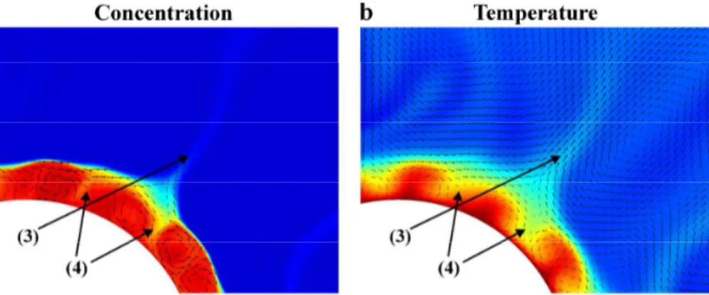
3. Thermal convection forming in the upper layer erodes the surface of the dense layer by viscous drag.

4. Inner convection within the dense layer intermixes light material from the overlying mantle.

Processes (1) and (2) result in the increase of the temperature diﬀerence between

5

the layers, the processes (3) and (4) cause the decrease of the concentration diﬀ er-ence. While the first two phenomena are constrained by the total temperature drop across the mantle (practically∆Tm/2, see Fig. 2b), the latter two are not. Erosion (3)

and dilution (4) gradually reduce the chemical density diﬀerence between the layers until the system reaches the instability point (Beﬀ=1) when mixing begins. Mixing oc-10

curs in every case, even if the time might exceed the Earth’s age (B≥1). Figure 3

illustrates the phenomena of the erosion and dilution of the dense layer in the con-centration and the temperature fields. Black arrows denote the mass flux of the dense material in Fig. 3a and the velocity of the flow in Fig. 3b.

We investigated how the occurrence time of the two most characteristic events (the

15

onset and the end of the eﬀective TCC) depends on the initial chemical density diﬀ er-ence,β(Fig. 4a). Obviously, largerβresults in more stable, long-lived dense layer and larger occurrence time. A parabolic relation was found between the occurrence time of

Beﬀ=1 (onset of mixing) andβ. Davaille (1999) observed a similar relation in her

labo-ratory experiments studying the eﬀect of the buoyancy ratio (and other parameters) on

20

the entrainment rate. Parabolic function fits well on data ofBeﬀ=0 (end of mixing) too.

As it was shown in Fig. 2, both the erosion/dilution phase (to stage c) and the eﬀ ec-tive TCC phase (between stage c and d) can be characterized by a linear decrease in

∆_c_{. The e}ﬀ_{ective buoyancy ratio displays a similar feature apart from its initial phase,}

which is due to the transient heating of the dense layer and the cooling of the overlying

25

mantle (from stage a to b). Figure 4b illustrates the slope of the linear curves fitted on

∆_c_and _B_e_ﬀ _{time series during the erosion/dilution phase. It is established that larger}

(10)

ec-SED

6, 2675–2697, 2014

A. Galsa et al.

Title Page

Tables Figures

◭ ◮

Back Close

Full Screen / Esc

Discussion

P

a

per

|

Discus

sion

P

a

per

|

Discussion

P

a

per

|

Discussion

P

a

per

|

tive erosion/dilution process. Figure 4b presents a power function relation between the slopes of time series (∆corBeﬀ) andβ. Both the parabolic relation in Fig. 4a and the

power function relation in Fig. 4b support the idea that mixing of the layers occurs for arbitrary density contrast. It is worth noting that the eﬀective TCC phase demonstrates also a linear decrease in ∆c and Beﬀ, but with steeper slope (Fig. 2). The slope of 5

the linear curves fitted on the time series shows a slight decrease asβincreases (not shown).

4 Discussion and conclusions

A new parameter, the eﬀective buoyancy ratio, Beﬀ was defined to characterize the

dynamics of thermo-chemical convection occurring in the Earth’s mantle. Buoyancy

10

ratio,B, in its classical meaning (Davaille et al., 2002) forecasts the resistivity of the dense layer against mixing, however it is insensitive to its behavior. Additionally, our calculations show that mixing also occurs in case of B >1 suggesting the instability of two-layer convection for arbitrary value of B (Davaille, 1999). On the other hand,

Beﬀ illustrates well the evolution of the initial dense layer above the CMB consisting 15

of four phases: (i) transition phase of warming dense layer; (ii) erosion and dilution of the dense layer; (iii) eﬀective thermo-chemical convection (mixing of layers); (iv) homogenization.

These conclusions were drawn from a simple isoviscous model. However, the TCC leading to the dissolution of the dense layer strongly depends on the

viscos-20

ity. Therefore, a more complex model including depth-, temperature- and composition-dependent viscosity and composition-composition-dependent internal heating was calculated in or-der to investigate the dynamics of the TCC and the variation of the eﬀective buoyancy ratio. Parameters controlling the viscosity and the internal heating were assigned based on the results of Deschamps and Tackley (2008, 2009). An Arrhenius-type law

deter-25

(11)

SED

6, 2675–2697, 2014

A. Galsa et al.

Title Page

Tables Figures

◭ ◮

Back Close

Full Screen / Esc

Discussion

P

a

per

|

Discus

sion

P

a

per

|

Discussion

P

a

per

|

Discussion

P

a

per

|

with the temperature. A viscosity jump with a factor of 30 was superimposed at the depth of 660 km reflecting the eﬀect of mineralogical phase change on the viscosity. The viscosity of the dense material (c=_{1) is half of that of the light material (}_c=₀₎

with a linear transition. Internal heating was adjusted to produce 65 mW m−2 average heat flux on the surface, but the heat production of the dense material was increased by

5

a factor of 10 due to the higher abundance of radioactive elements. The initial compo-sitional density contrast between the layers wasβ=_{6 % correspondingly to the model}

presented in Fig. 1. Simulation started from a quasi-stationary state of the temperature field obtained from a chemically homogeneous, purely thermal convection model with depth- and temperature-dependent viscosity and homogeneous internal heating.

10

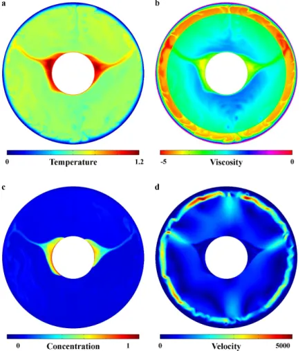
Figure 5 illustrates the pattern of the TCC for the complex model at 3.5 Gyr after the inset of the dense layer when the eﬀective buoyancy ratio is approx. 1.13. Dur-ing 3.5 Gyr the dense layer disintegrated and two hot, compositionally dense, nearly antipodal piles formed with sharp sides. Due to the concentration-dependent internal heating the temperature within piles exceeds the CMB temperature thus the

viscos-15

ity decreases considerably. The concentration and velocity field attest that a sluggish internal convection forms within the piles. A stagnant lid regime evolved owing to the strongly temperature-dependent viscosity (Solomatov, 1995) which does not partici-pate in the convection. Beneath the stagnant lid vivid small-scale convection occurs in the upper mantle (Kuslits et al., 2014). Due to the lack of the endothermic phase

tran-20

sition advective mass and heat transport exists between the upper and lower mantle. Figure 2 displays the variation of the concentration and temperature diﬀerences be-tween the layers and the eﬀective buoyancy ratio for the “mantle-like” model (mm_6 %). As a consequence of the stagnant lid regime∆T decreased compared to the isovis-cous case but the character of the curve remained similar. The rate of the decrease in

25

∆_c_{by erosion and dilution processes became steeper owing to the reduced viscosity}

(12)

SED

6, 2675–2697, 2014

A. Galsa et al.

Title Page

Tables Figures

◭ ◮

Back Close

Full Screen / Esc

Discussion

P

a

per

|

Discus

sion

P

a

per

|

Discussion

P

a

per

|

Discussion

P

a

per

|

and internal heating was reduced compared to isoviscous model by about 20 %, but the physical processes acting in the two models were the same.

In order to make a comparison among diﬀerent numerical models Tackley (2012) rescaled the results for the heat expansion ofα=₁₀−5

1 K−1, as a more realistic value in the deep, compressible mantle (Mosenfelder et al., 2009). Applying smaller heat

5

expansion requires less initial compositional density contrast to obtain the sameBeﬀ.

Rescaling our model (Fig. 1) for reduced heat expansion minimumβ=_{3 % initial}

com-positional density contrast is needed to maintain the dense layer over the age of the Earth. It is in accordance with the results of Tackley (2012) who arrived to density diﬀerence of 2–3 % based on diﬀerent model calculations.

10

Trampert et al. (2004) using tomographic likelihoods separated the total density vari-ation in the mantle into temperature and chemical density varivari-ation. They established that the present compositional density variation is dominant in the lower 1000 km of mantle and it is likely to exceed 2 %. It corresponds to our models with initial density contrast ofβ=3 % assuming reduced heat expansion, because the density diﬀerence

15

decreases gradually due to erosion and dilution processes (Fig. 2).

Several normal modes of the Earth show a significant sensitivity to the density/shear velocity ratio in the deep mantle (Koelemeijer et al., 2012). Ishi and Tromp (2004) re-vealed a total density increment of approx. 0.5 % beneath Africa and Pacific in which the opposite eﬀect of the temperature and the compositional variation is superimposed.

20

Taking into account that the compositional density increase of more than 2 % and the total density increase of only 0.5 % a rough estimate of the eﬀective buoyancy ratio gives a value of slightly above 1. Based on our model results at this stage the TCC system in the Earth’s mantle might be just before the instability point. It agrees well with the present strongly deformed, disintegrated morphology of LLSVPs (e.g.

Gar-25

nero et al., 2007a).

(13)

SED

6, 2675–2697, 2014

A. Galsa et al.

Title Page

Tables Figures

◭ ◮

Back Close

Full Screen / Esc

Discussion

P

a

per

|

Discus

sion

P

a

per

|

Discussion

P

a

per

|

Discussion

P

a

per

|

Acknowledgements. The authors are grateful to Paul J. Tackley for his constructive remarks. This research was supported by the European Union and the State of Hungary, co-financed by the European Social Fund in the framework of TÁMOP 4.2.4. A/1-11-1-2012-0001 “National Excellence Program”. This research was also supported by the Hungarian Scientific Research Fund (OTKA K-72665 and OTKA NK100296) and it was implemented thanks to the scholarship

5

in the framework of the TÁMOP 4.2.4.A-1 priority project.

References

Bull, A. L., McNamara, A. K., and Ritsema, J.: Synthetic tomography of plume clusters and thermochemical piles, Earth Planet. Sc. Lett., 278, 152–162, 2009.

Chandrasekhar, S.: Hydrodynamic and Hydromagnetic Stability, Clarendon, Oxford, 1961.

10

Christensen, U. R. and Yuen, D. A.: The interaction of a subducting lithospheric slab with a chemical or phase boundary, J. Geophys. Res., 89, 4389–4402, 1984.

Č_íž_{ková, H. and Matyska, C.: Layered convection with an interface at a depth of 1000 km:} stability and generation of slab-like downwellings, Phys. Earth Planet. In., 141, 269–279, 2004.

15

Davaille, A.: Two-layer thermal convection in miscible viscous fluids, J. Fluid Mech., 379, 223– 253, 1999.

Davaille, A., Girard, F., and Le Bars, M.: How to anchor hotspots in a convecting mantle?, Earth Planet. Sc. Lett., 203, 621–634, 2002.

Deschamps, F. and Tackley, P. J.: Searching for models of thermo-chemical convection that

20

explain probabilistic tomography I – principles and influence of rheological parameters, Phys. Earth Planet. In., 171, 357–373, 2008.

Deschamps, F. and Tackley, P. J.: Searching for models of thermo-chemical convection that explain probabilistic tomography II – influence of physical and compositional parameters, Phys. Earth Planet. In., 176, 1–18, 2009.

25

Dziewonski, A. M., Foret, A. M., Su, W.-J., and Woodward, R. L.: Seismic tomography and geo-dynamics, in: Relating Geophysical Structures and Processes, The Jeﬀreys Volume, AGU Geophysical Monograph, 76, Washington, DC, 67–105, 1993.

Ford, S. R., Garnero, E. J., and McNamara, A. K.: A strong lateral shear velocity gradient and anisotropy heterogeneity in the lowermost mantle beneath the southern Pacific, J. Geophys.

30

(14)

SED

6, 2675–2697, 2014

A. Galsa et al.

Title Page

Tables Figures

◭ ◮

Back Close

Full Screen / Esc

Discussion

P

a

per

|

Discus

sion

P

a

per

|

Discussion

P

a

per

|

Discussion

P

a

per

|

Garnero, E. J. and McNamara, A. K.: Structure and dynamics of Earth’s lower mantle, Science, 320, 626–628, 2008.

Garnero, E. J., Thorne, M. S., McNamara, A. K., and Rost, S.: Fine-scale ultra-low velocity zone layering at the core-mantle boundary and superplumes, in: Superplumes, Springer, 139–158, 2007a.

5

Garnero, E. J., Lay, T., and McNamara, A. K.: Implications of lower-mantle structural hetero-geneity for existence and nature of whole-mantle plumes, in Plates, plumes, and planetary processes, Geol. Soc. Am. Special Paper, 79–101, doi:10.1130/2007.2430(05), 2007b. Hansen, U. and Yuen, D. A.: Numerical simulations of thermal-chemical instabilities at the core–

mantle boundary, Nature, 334, 237–240, 1988.

10

Ishii, M. and Tromp, J.: Constraining large-scale mantle heterogeneity using mantle and inner-core sensitive normal modes, Phys. Earth Planet. In., 146, 113–124, 2004.

Jellinek, A. M. and Manga, M.: The influence of a chemical boundary layer on the fixity, spacing and lifetime of mantle plumes, Nature, 418, 760–763, 2002.

Koelemeijer, P. J., Deuss, A., and Trampert, J.: Normal mode sensitivity to Earth’s D′′

layer and

15

topography on the core-mantle boundary: what we can and cannot see, Geophys. J. Int., 190, 553–568, 2012.

Kuslits, L. B., Farkas, M. P., and Galsa, A.: Eﬀect of temperature-dependent viscosity on mantle convection, Acta Geod. Geophys., 49, 249–263, doi:10.1007/s40328-014-0055-7, 2014. Lay, T.: The deep mantle thermo-chemical boundary layer: The putative mantle plume source,

20

in: Plates, Plumes, and Paradigms, Geol. Soc. Am. Bull., 338, 193–205, 2005.

Lay, T., Hernlund, J., Garnero, E. J., and Thorne, M. S.: A post-perovskite lens and D′′heat flux beneath the Central Pacific, Science, 314, 1272–1276, 2006.

Lin, S.-C. and Van Keken, P. E.: Dynamics of thermochemical plumes: 1. Plume for-mation and entrainment of a dense layer, Geochem. Geodyn. Geosyst., 7, Q02006,

25

doi:10.1029/2005GC001071, 2006.

Masters, G., Laske, G., Bolton, H., and Dziewonski, A. M.: The relative behavior of shear ve-locity, bulk sound speed, and compressional velocity in the mantle: implications for chemical and thermal structure in Earth’s deep interior, in: Mineral Physics and Tomography From the Atomic to the Global Scale, AGU, Washington, DC, 63–87, 2000.

30

(15)

SED

6, 2675–2697, 2014

A. Galsa et al.

Title Page

Tables Figures

◭ ◮

Back Close

Full Screen / Esc

Discussion

P

a

per

|

Discus

sion

P

a

per

|

Discussion

P

a

per

|

Discussion

P

a

per

|

Mégnin, C. and Romanowicz, B.: The three-dimensional shear-velocity structure of the mantle from the inversion of body, surface and higher-mode waveforms, Geophys. J. Int., 143, 709– 728, 2000.

Mosenfelder, J. L., Asimow, P. D., Frost, D. J., Rubie, D. C., and Ahrens, T. J.: The MgSiO₃ system at high pressure: thermodynamic properties perovskite, postperovskite, and melt

5

from global inversion of shock and static compression data, J. Geophys. Res., 114, B01203, doi:10.1029/2008JB005900, 2009.

Nakagawa, T. and Tackley, P. J.: Eﬀect of thermo-chemical mantle convection on the thermal evolution of the Earth’s core, Earth Planet. Sc. Lett., 220, 107–119, 2004.

Ni, S., Tan, E., Gurnis, M., and Helmberger, D. V.: Sharp sides to the African superplume,

10

Science, 296, 1850–1852, 2002.

Sleep, N. H.: Gradual entrainment of a chemical layer at the base of the mantle by overlying convection, Geophys. J., 95, 437–447, 1988.

Solomatov, V. S.: Scaling of temperature- and stress-dependent viscosity convection, Phys. Fluids, 7, 266–274, 1995.

15

Tackley, P. J.: Dynamics and evolution of the deep mantle resulting from thermal, chemical, phase and melting eﬀects, Earth-Sci. Rev., 110, 1–25, 2012.

Thorne, M. S., Garnero, E. J., and Grand, S. P.: Geographic correlation between hot spots and deep mantle lateral shear-wave velocity gradients, Phys. Earth Planet. In., 146, 47–63, 2004.

20

Torsvik, T. H., Burke, K., Steinberger, B., Webb, S. J., and Ashwal, L. D.: Diamonds sampled by plumes from the core-mantle boundary, Nature, 466, 352–355, 2010.

Trampert, J., Deschamps, F., Resovsky, J., and Yuen, D. A.: Probabilistic tomography maps chemical heterogeneities throughout the lower mantle, Science, 306, 853–856, 2004. Van Keken, P.: Cylindrical scaling for dynamical cooling models of the Earth, Phys. Earth Planet.

25

In., 124, 119–130, 2001.

Wang, Y. and Wen, L.: Mapping the geometry and geographic distribution of a very low velocity province at the base of the Earth’s mantle, J. Geophys. Res., 109, B10305, doi:10.1029/2003JB002674, 2004.

Zhao, D.: Multiscale seismic tomography and mantle dynamics, Gondwana Res., 15, 297–323,

30

2009.

(16)

SED

6, 2675–2697, 2014

A. Galsa et al.

Title Page

Tables Figures

◭ ◮

Back Close

Full Screen / Esc

Discussion

P

a

per

|

Discus

sion

P

a

per

|

Discussion

P

a

per

|

Discussion

P

a

per

|

(17)

SED

6, 2675–2697, 2014

A. Galsa et al.

Title Page

Tables Figures

◭ ◮

Back Close

Full Screen / Esc

Discussion

P

a

per

|

Discus

sion

P

a

per

|

Discussion

P

a

per

|

Discussion

P

a

per

|

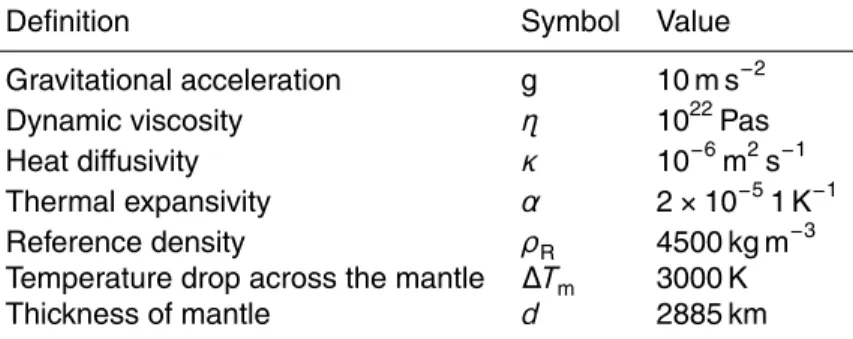
Table 1.Model constants.

Definition Symbol Value

Gravitational acceleration g 10 m s−2

Dynamic viscosity η 1022Pas

Heat diﬀusivity κ 10−6m2s−1

Thermal expansivity α 2×10−51 K−1

Reference density ρ_R 4500 kg m−3

Temperature drop across the mantle ∆T_m 3000 K

(18)

SED

6, 2675–2697, 2014

A. Galsa et al.

Title Page

Tables Figures

◭ ◮

Back Close

Full Screen / Esc

Discussion

P

a

per

|

Discus

sion

P

a

per

|

Discussion

P

a

per

|

Discussion

P

a

per

|

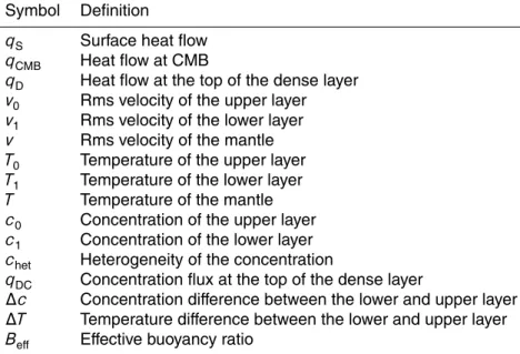
Table 2.Monitoring parameters.

Symbol Definition

qS Surface heat flow qCMB Heat flow at CMB

qD Heat flow at the top of the dense layer v₀ Rms velocity of the upper layer

v₁ Rms velocity of the lower layer

v Rms velocity of the mantle

T₀ Temperature of the upper layer

T₁ Temperature of the lower layer

T Temperature of the mantle

c₀ Concentration of the upper layer

c₁ Concentration of the lower layer

c_het Heterogeneity of the concentration

q_DC Concentration flux at the top of the dense layer

∆_c Concentration diﬀerence between the lower and upper layer ∆_T Temperature diﬀerence between the lower and upper layer

(19)

SED

6, 2675–2697, 2014

A. Galsa et al.

Title Page

Tables Figures

◭ ◮

Back Close

Full Screen / Esc

Discussion

P

a

per

|

Discus

sion

P

a

per

|

Discussion

P

a

per

|

Discussion

P

a

per

|

re 1 Five stages characterizing the evolution of the thermo-chemical convection.

(20)

SED

6, 2675–2697, 2014

A. Galsa et al.

Title Page

Tables Figures

◭ ◮

Back Close

Full Screen / Esc

Discussion

P

a

per

|

Discus

sion

P

a

per

|

Discussion

P

a

per

|

Discussion

P

a

per

|

(21)

SED

6, 2675–2697, 2014

A. Galsa et al.

Title Page

Tables Figures

◭ ◮

Back Close

Full Screen / Esc

Discussion

P

a

per

|

Discus

sion

P

a

per

|

Discussion

P

a

per

|

Discussion

P

a

per

|

(22)

SED

6, 2675–2697, 2014

A. Galsa et al.

Title Page

Tables Figures

◭ ◮

Back Close

Full Screen / Esc

Discussion

P

a

per

|

Discus

sion

P

a

per

|

Discussion

P

a

per

|

Discussion

P

a

per

|

Figure 4 (a) Occurrence time of the two most characteristic events: =1 (onset of mixing)

Figure 4. (a)Occurrence time of the two most characteristic events:B_eﬀ=1 (onset of mixing)

andB_eﬀ=0 (end of mixing) as well as(b)slope of the decrease of the concentration diﬀerence

(23)

SED

6, 2675–2697, 2014

A. Galsa et al.

Title Page

Tables Figures

◭ ◮

Back Close

Full Screen / Esc

Discussion

P

a

per

|

Discus

sion

P

a

per

|

Discussion

P

a

per

|

Discussion

P

a

per

|

gure 5 A quasi-stationary state of the (a) temperature, (b) viscosity, (c) concentration of